An Active Contour Algorithm
THOMAS A. LAMPERT
Ph.D. Thesis
This thesis is submitted in partial fulfilment of the requirements for the degree of Doctor of Philosophy.
Advanced Computer Architecture Group Department of Computer Science
United Kingdom
In many areas of science, near-periodic phenomena represent important information within
time-series data. This thesis takes the example of the detection of non-transitory frequency com-ponents in passive sonar data, a problem which finds many applications. This problem is typically
transformed into the pattern recognition domain by representing the time-series data as a
spectro-gram, in which slowly varying periodic signals appear as curvilinear tracks.
The research is initiated with a survey of the literature, which is focused upon research into the
detection of tracks within spectrograms. An investigation into low-level feature detection reveals
that none of the evaluated methods perform adequately within the low signal-to-noise ratios of real-life spectrograms and, therefore, two novel feature detectors are proposed. An investigation into
the various sources of information available to the detection process shows that the most simple
of these, the individual pixel intensity values, used by most existing algorithms, is not sufficient for the problem. To overcome these limitations, a novel low-level feature detector is integrated
into a novel active contour track detection algorithm, and this serves to greatly increase detection
rates at low signal-to-noise ratios. Furthermore, the algorithm integrates a priori knowledge of the harmonic process, which describes the relative positions of tracks, to augment the available
information in difficult conditions.
Empirical evaluation of the algorithm demonstrates that it is effective at detecting tracks at signal-to-noise ratios as low as:0.5dB with vertical;3dB with oblique; and2dB with sinusoidal variation of harmonic features. It is also concluded that the proposed potential energy increases
the active contour’s effectiveness in detecting all the track structures by a factor of eight (as de-termined by the line location accuracy measure), even at relatively high signal-to-noise ratios,
and that incorporating a priori knowledge of the harmonic process increases the detection rate
by a factor of two.
List of Tables 9
List of Figures 11
List of Algorithms 15
1 Introduction 23
1.1 The Passive Sonar Problem . . . 25
1.2 Data . . . 26
1.2.1 Signal Generation . . . 26
1.2.2 Signal Propagation . . . 28
1.2.3 Spectrogram Formation . . . 29
1.3 Thesis Contributions . . . 33
1.4 Thesis Structure . . . 34
2 The Field as it Stands 35 2.1 Definition of Evaluation Criteria . . . 35
2.2 Algorithm Taxonomy . . . 37
2.3 Literature Survey . . . 37
2.3.1 Maximum Likelihood Estimators . . . 37
2.3.2 Image Processing . . . 39
2.3.2.1 Two-Pass Split-Window . . . 40
2.3.2.2 Edge Detection . . . 40
2.3.2.3 Likelihood Ratio Test . . . 41
2.3.2.4 Multi-Stage Decision Process . . . 42
2.3.2.5 Steerable Filter . . . 43
2.3.3 Neural Networks . . . 44
2.3.3.1 Supervised Learning . . . 44
2.3.3.2 Unsupervised Learning . . . 48
2.3.4 Statistical Models . . . 49
2.3.4.1 Dynamic Programming . . . 49
2.3.4.2 Hidden Markov Model . . . 49
2.3.5 Tracking Algorithms . . . 53
2.3.5.1 Particle Filter . . . 53
2.3.6 Relaxation Methods . . . 54
2.3.6.1 Simulated Annealing . . . 54
2.3.7 Expert Systems . . . 55
2.4 Discussion . . . 56
2.4.1 Algorithm Evaluation . . . 56
2.4.2 Technique Limitations . . . 56
2.5 Research Directions . . . 59
2.6 Conclusions . . . 60
3 Low-Level Feature Detection 61 3.1 ‘Optimal’ Feature Detectors . . . 62
3.1.1 Bayesian Inference . . . 63
3.1.1.1 Intensity Distribution Models . . . 63
3.1.1.2 Decision Rules . . . 65
3.1.2 Bayesian Inference using Spatial Information . . . 66
3.1.2.1 Window Function . . . 67
3.1.2.2 Decision Rules . . . 68
3.1.3 Bar Detector . . . 68
3.1.3.1 Length Search . . . 70
3.2 ‘Sub-Optimal’ Feature Detectors . . . 71
3.2.1 Data-Based Subspace Learning . . . 72
3.2.1.1 Explicit Dimension Reduction . . . 72
3.2.1.2 Implicit Dimension Reduction . . . 74
3.2.1.3 Classification Methods . . . 75
3.2.2 Model-Based Subspace Learning . . . 78
3.3 Evaluation of Feature Detectors . . . 79
3.3.1 Experimental Data . . . 80
3.3.2 Results . . . 81
3.3.2.1 Comparison of ‘Optimal’ Detection Methods . . . 82
3.3.2.2 Comparison of ‘Sub-Optimal’ Detection Methods . . . 84
3.4 Harmonic Integration . . . 84
3.4.1 Results . . . 85
3.5 Summary . . . 86
4 A Track Detection Algorithm 89 4.1 The Active Contour Algorithm . . . 90
4.1.1 Algorithm Background . . . 91
4.1.1.1 Contour Initialisation . . . 91
4.1.1.2 Potential Energy . . . 92
4.1.1.3 Internal Energy . . . 93
4.1.1.5 Multiple Contours . . . 95
4.2 Track Detection Framework . . . 95
4.2.1 Gradient Potential . . . 95
4.2.2 Potential Energy . . . 96
4.2.2.1 Noise Model Training . . . 97
4.2.2.2 Individual Track Detection . . . 99
4.2.2.3 Multiple Track Detection . . . 100
4.2.2.4 Noise Model . . . 101
4.2.3 Internal Energy . . . 102
4.2.4 Energy Minimisation . . . 105
4.2.4.1 A Note on the Vertices’ Neighbourhood . . . 107
4.2.5 Rolling Window . . . 107
4.3 Complexity Analysis . . . 109
4.3.1 Original Internal Energy . . . 109
4.3.2 Perrin Internal Energy . . . 110
4.4 Summary . . . 110
5 Algorithm Evaluation 113 5.1 Evaluation Measure . . . 114
5.1.1 Experimental Data . . . 114
5.2 Parameter Selection . . . 115
5.3 Comparison of Internal Energies . . . 116
5.3.1 Parameter Sensitivity . . . 117
5.3.2 Performance . . . 119
5.3.3 Discussion . . . 124
5.4 Original Potential Energy . . . 125
5.4.1 Parameter Sensitivity . . . 125
5.4.2 Performance . . . 126
5.5 Multiple Versus Individual Track Detection . . . 127
5.5.1 Performance . . . 129
5.5.2 Discussion . . . 131
5.6 Further Discussion . . . 132
5.6.1 Active Contour Algorithm . . . 132
5.6.2 Relation to Existing Methods . . . 133
5.6.3 Line Location Accuracy . . . 134
5.7 Summary . . . 135
6 Conclusions 137 6.1 Future Work . . . 141
6.1.1 Track Association . . . 141
6.1.2 Ambient Noise . . . 141
6.1.4 Automatic Determination of Harmonic Features . . . 143
A Additional Diagrams 145 A.1 Chapter 3 . . . 145
A.2 Chapter 5 . . . 147
A.2.1 Perrin Internal Energy and the Proposed Potential Energy . . . 147
A.2.2 Original Internal Energy and the Proposed Potential Energy . . . 152
A.2.3 Original Internal Energy and the Original Potential Energy . . . 157
A.2.4 Single Track Detection . . . 162
A.2.5 Example Detections . . . 167
A.2.6 Standard Deviations . . . 169
List of References 177
Author Index 193
2.1 Track characteristics and application criteria of track detection algorithms. . . 36
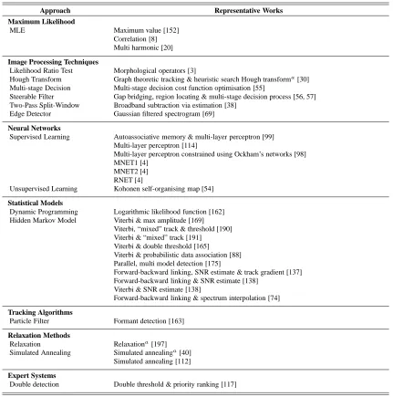
2.2 Categorisation of spectrogram track detection techniques. . . 38
2.3 Analysis of spectrogram track detection algorithms. . . 57
3.1 Classification percentages using the proposed features. . . 77
3.2 Classification standard deviations using the proposed features. . . 77
3.3 Parameter values spanning the synthetic data set. . . 80
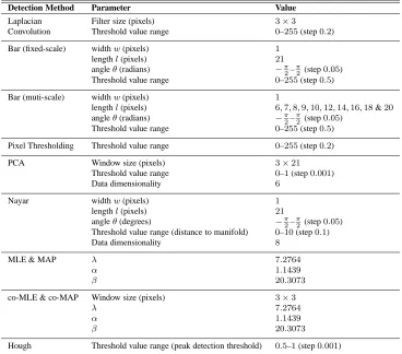
3.4 Parameter values of each detection method used in the experimentation. . . 82
A.1 The standard deviation of the mean training line location accuracies—a compari-son between internal energies. . . 169
A.2 The standard deviations of the vertical track mean line location accuracies—a comparison between internal energies. . . 170
A.3 The standard deviations of the oblique track mean line location accuracies—a comparison between internal energies. . . 170
A.4 The standard deviations of the sinusoidal (ten second period) track mean line lo-cation accuracies—a comparison between internal energies. . . 171
A.5 The standard deviations of the sinusoidal (fifteen second period) track mean line location accuracies—a comparison between internal energies. . . 172
A.6 The standard deviations of the sinusoidal (twenty second period) track mean line location accuracies—a comparison between internal energies. . . 173
A.7 The standard deviation of the mean training line location accuracies—single track detection. . . 173
A.8 The standard deviations of the vertical track mean line location accuracies—single track detection. . . 173
A.9 The standard deviations of the oblique track mean line location accuracies—single track detection. . . 174
A.10 The standard deviations of the sinusoidal (ten second period) track mean line lo-cation accuracies—single track detection. . . 174
A.11 The standard deviations of the sinusoidal (fifteen second period) track mean line location accuracies—single track detection. . . 174
1.1 Flow diagram of the passive sonar process. . . 25
1.2 Magnitude Squared of the Fourier transform of acoustic signal. . . 30
1.3 Spectrogram image. . . 31
1.4 Synthetic spectrogram examples. . . 32
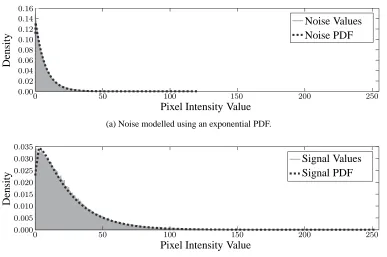
3.1 Class-conditional probability density function class fittings. . . 64
3.2 Pixel likelihood values. . . 66
3.3 Maximum likelihood spectrogram pixel classification. . . 67
3.4 The bar operator. . . 69
3.5 The mean response of the rotated bar operator centred upon a vertical line. . . 70
3.6 Windowed spectrogram PCA eigenvalues. . . 73
3.7 Windowed spectrogram projected onto the first two principal components. . . 74
3.8 Windowed spectrogram LDA eigenvalues. . . 74
3.9 Windowed spectrogram projected onto the first two LDA principal components. . 75
3.10 Results of the bar and parametric manifold detection methods. . . 78
3.11 The effects of the parameter values upon the appearance of sinusoidal tracks. . . 81
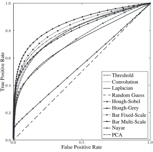
3.12 ROC curves of the evaluated detection methods. . . 83
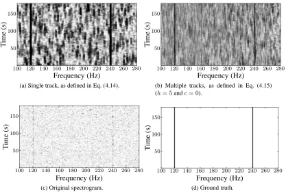
3.13 The result of the harmonic transform applied to a spectrogram. . . 84
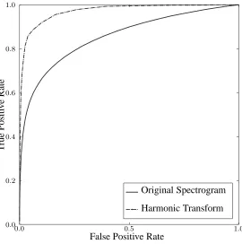
3.14 ROC curves of the bar detector with and without harmonic integration. . . 86
4.1 Windowed feature vectors projected onto two principal components. . . 98
4.2 Potential energy topologies for a180×180pixel section of a spectrogram. . . . 99
4.3 The contour mesh. . . 101
4.4 The original internal energies’ values when modelling a straight vertical track. . . 103
4.5 The original internal energies’ values when modelling an oblique track. . . 103
4.6 The original internal energies’ values when modelling a sinusoidal track. . . 103
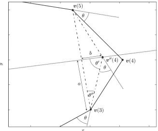
4.7 The optimal contour vertex position as defined by the Perrin internal energy. . . . 104
5.1 The eigenvalues associated with the principal components. . . 116
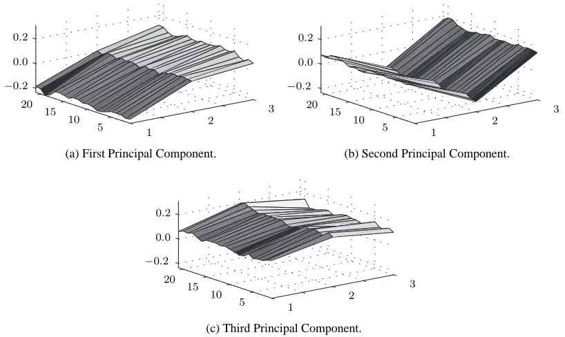
5.2 The first three principal components viewed as3×21point surface plots. . . 116
5.3 Mean training line location accuracies as functions of parameter values—a com-parison between internal energies. . . 118
5.4 Vertical track mean line location accuracies as functions of SNR—a comparison between internal energies. . . 120
5.5 Oblique track mean line location accuracies as functions of SNR—a comparison
between internal energies. . . 121
5.6 Sinusoidal (ten second period) track mean line location accuracies as functions of SNR—a comparison between internal energies. . . 122
5.7 Sinusoidal (fifteen second period) track mean line location accuracies as functions
of SNR—a comparison between internal energies. . . 123
5.8 Sinusoidal (twenty second period) track mean line location accuracies as functions
of SNR—a comparison between internal energies. . . 124
5.9 Mean training line location accuracies as functions of parameter values—original potential energy. . . 126
5.10 Vertical track mean line location accuracies as functions of SNR—original
poten-tial energy. . . 127
5.11 Oblique track mean line location accuracies as functions of SNR—original poten-tial energy. . . 127
5.12 Sinusoidal track mean line location accuracies as functions of SNR—original
po-tential energy. . . 128
5.13 Mean training line location accuracy as a function of the gradient potential’s para-meter values—single track detection. . . 129
5.14 Vertical track mean line location accuracies as functions of SNR—single track
detection. . . 129
5.15 Oblique track mean line location accuracies as functions of SNR—single track
detection. . . 130 5.16 Sinusoidal (ten second period) track mean line location accuracies as functions of
SNR—single track detection. . . 130
5.17 Sinusoidal (fifteen second period) track mean line location accuracies as functions
of SNR—single track detection. . . 131
5.18 Sinusoidal (twenty second period) track mean line location accuracies as functions of SNR—single track detection. . . 131
6.1 An example of real-world track detection. . . 140
A.1 PCA low-level feature detection performance as functions of SNR. . . 145
A.2 PCA low-level feature detection performance as a function of the window’s height
and width. . . 146
A.3 Mean training true positive and false positive detections as functions of parameter values—Perrin internal energy. . . 147
A.4 Vertical track mean true positive and false positive detections as functions of SNR—
Perrin internal energy. . . 148
A.6 Sinusoidal (ten second period) track mean true positive and false positive detec-tions as funcdetec-tions of SNR—Perrin internal energy. . . 149
A.7 Sinusoidal (fifteen second period) track mean true positive and false positive
de-tections as functions of SNR—Perrin internal energy. . . 150
A.8 Sinusoidal (twenty second period) track mean true positive and false positive
de-tections as functions of SNR—Perrin internal energy. . . 151
A.9 Mean training true positive and false positive detections as functions of parameter
values—original internal energy. . . 152
A.10 Vertical track mean true positive and false positive detections as functions of SNR—
original internal energy. . . 153
A.11 Oblique track mean true positive and false positive detections as functions of SNR—original internal energy. . . 153
A.12 Sinusoidal (ten second period) track mean true positive and false positive detec-tions as funcdetec-tions of SNR—original internal energy. . . 154
A.13 Sinusoidal (fifteen second period) track mean true positive and false positive de-tections as functions of SNR—original internal energy. . . 155
A.14 Sinusoidal (twenty second period) track mean true positive and false positive
de-tections as functions of SNR—original internal energy. . . 156
A.15 Mean training true positive and false positive detections as functions of parameter
values—original potential energy. . . 157
A.16 Vertical track mean true positive and false positive detections as functions of SNR—
original potential energy. . . 158
A.17 Oblique track mean true positive and false positive detections as functions of
SNR—original potential energy. . . 158
A.18 Sinusoidal (ten second period) track mean true positive and false positive detec-tions as funcdetec-tions of SNR—original potential energy. . . 159
A.19 Sinusoidal (fifteen second period) track mean true positive and false positive de-tections as functions of SNR—original potential energy. . . 160
A.20 Sinusoidal (twenty second period) track mean true positive and false positive
de-tections as functions of SNR—original potential energy. . . 161
A.21 Mean training true positive and false positive detections as a function of the
gra-dient potential’s parameter values—single track detection. . . 162
A.22 Vertical track mean true positive and false positive detections as functions of SNR—
single track detection. . . 163
A.23 Oblique track mean true positive and false positive detections as functions of
SNR—single track detection. . . 163
A.24 Sinusoidal (ten second period) track mean true positive and false positive
detec-tions as funcdetec-tions of SNR—single track detection. . . 164
A.26 Sinusoidal (twenty second period) track mean true positive and false positive de-tections as functions of SNR—single track detection. . . 166
A.27 A set of example detections. . . 167
3.1 Bar length binary search . . . 71
4.1 Contour energy minimisation . . . 106
The time spent researching and documenting my Ph.D. has been both exciting and tumultuous.
Many people have supported me, both academically and personally. There are many with whom I have had mere incidences, however, they have all, in some way, influenced that which is presented
in front of you now. If I try to list all the people who have influenced my work, I will fail, and I
therefore list those which are, for one reason or another, most prominent in my mind.
Needless to say, the academic content of this thesis has been primarily shaped by my
supervi-sor, Dr. Simon O’Keefe, whose knowledge, guidance, encouragement, and support have allowed
me to produce this document of my journey and to become an independent researcher. Dr. Nick Pears and Dr. Richard Harvey have both read, understood, and examined me upon its content and
I greatly appreciate their dedication to the academic standard which has instilled a measure of
self-confidence in my work. Whilst elucidating the problems tackled by this research I was very fortunate to have the practical and theoretical guidance of Jim Nicholson, who I would also like to
thank for his finely tuned sense for grammatical correctness. Furthermore, Dr. Duncan Williams
has supported my research and encouraged its dissemination and continuation. Filo Ottaway has always demonstrated a dedication to the students of this department, far beyond that which could
be expected of her. I appreciate the encouragement, support, friendship, and dedication that she has given me. To all of the academic, administrative and industrial supporters who have encouraged
me during the past four years, I am deeply grateful. I would also like to acknowledge the
inspi-rational teachers and academics who have encouraged and contributed to my earlier education, in particular: Ms. Henderson, Mrs. Smith, Mrs. Mills, Mr. McPherson, and Prof. Everson.
My experience of Ph.D. studies leads me to believe that it is not only a journey of which the
goal is to reach an understanding of research and science but that it is also a medium through which it is possible to gain a deeper understanding of oneself. As such, it is not only an exciting
and enjoyable experience but it can also present worrying and disorienting challenges, and this is
where the limitation of academic support is surpassed by that of family and friends. My parents, Andrew and Kathryn Lampert, have, throughout my life, provided me with the best possible
sup-port, encouragement and love, as has my sister, Harriet Lampert. I am grateful to them for all
the moments that I have spent at home over the previous four years, where I have been able to relax and enjoy times away from the pressure of work. Whilst there, many days have been spent
relaxing and contemplatively discussing thoughts next to rivers in the Cambridgeshire fens, fishing
with my dear friend Dan Fordham. When I was in need of escape I could always rely on another close friend Olivier Guillemot to help me recover perspective. It was during one such adventure
supportive people. Marcelo Romero has been a good friend since my first months here and has
supported me, both academically and personally, throughout my research. Eliza has punctuated my day with all manner of interesting discussion and has brightened up, what would otherwise
be, a dull office. Leo Freitas has been a true friend, with whom I have had many discussions and
memorable nights in various bars and pubs of York drinking the fine beer of the city. Every time that we play I am grateful to my friends who are the members of Saville Law; Andre, Leandro and
Lorenzo, with whom I have a means of unconstrained expression; I have truly enjoyed what we have together. I would like to thank Burcu Can for our discussions, photography, and her delightful
cooking. Frank Zeyda has encouraged my abilities in music and with whom I have enjoyed drinks,
discussions and parties. Pierre Andrews is someone who has helped me in my work, has been a friend, and who has almost killed me in the Alps, we have spent some unique moments together on
some spectacular adventures. I would particularly like to emphasise my fortune with the random
events that have resulted in my friendship with Bere. There is no doubt that she has unselfishly offered me far more than anyone could ever wish for, I am happy to have spent every moment that
we have had together, with such a kind person—mi amiga querida. Clarisse has been an extremely
kind friend, I have enjoyed her excellent culinary skills, and she has supported me when I needed it most. Silvana, housed me when I was homeless and has been an excellent, attentive friend, I
wish her luck with her future endeavours. Laure injected a little French madness into my life,
merci mon petit Franc¸ais. I thank Juan for distracting me from work with educational debates,
of sorts. Isabelle for our bucolic adventures. Malihe for forcing me to dance. Berna has, well,
been Berna, and it has been fantastic to know her. During my days in the lab, the most enjoyable
parts have been spent over lunch, the food was not so good, but the company transformed these times into something to look forward to, for this I would also like to thank Napol, Tobias, Simon,
Jos´e, and Marek. Furthermore, I would like to thank: Richard, Osmar, Simone, Lichi, Ahmad,
Shailesh, Peng, Lin, and Ping, for making the department a more interesting place to be, each in your own particular way; Guy, George, Stewart, Alan, and Saira, for our times in Manchester; and
Julia, Dan, Katharina, Valentina, Gioia, and Angelika, for our adventures in Spain. Finally, I
can-not finish these acknowledgements without expressing my appreciation for Tatjana, her dedication to helping me complete this thesis, her love, and her unbridled support during my most difficult
moments, have brought respite during the past year.
As I write these acknowledgements, I come to realise that the work presented here represents
far more than a mere document of my research. To all of the uniquely interesting people that I
through academia.
Parts of the following research have been previously presented or published in:
• Lampert T. and O’Keefe, S., 2010. An Active Contour Model for Spectrogram Track
De-tection. Pattern Recognition Letters 31(10), 1201–1206.
• Lampert T. and O’Keefe, S., February 2010. A Survey of Spectrogram Track Detection Algorithms. Applied Acoustics 71(2), 87–100.
• Lampert T. and O’Keefe, S., ‘Machine Learning of Harmonic Relationships which Maxi-mise Source Detection and Discrimination’, NATO & DSTL Workshop on Machine
Intelli-gence for Autonomous Operations, Lerici, Italy, October 7–8, 2009.
• Lampert, T., Pears, N. and O’Keefe, S., 2009. A Multi-Scale Piecewise Linear Feature
De-tector for Spectrogram Tracks. In: Proceedings of the IEEE 6th International Conference on
Advanced Video and Signal Based Surveillance. pp. 330–335, Genoa, Italy, September 2–4.
• Lampert, T., O’Keefe, S. and Pears, N., 2009. Line Detection Methods for Spectrogram
Images. In: Proceedings of 6th International Conference on Computer Recognition Systems.
Vol. 57 of Advances in Intelligent and Soft Computing, Springer, pp. 127–134.
• Lampert, T. and O’Keefe, S., 2009. A Comparison Framework for Spectrogram Track De-tection Algorithms. In: Proceedings of 6th International Conference on Computer
Recogni-tion Systems. Vol. 57 of Advances in Intelligent and Soft Computing, Springer, pp. 119–126.
• Lampert, T. and O’Keefe, S., 2008. Active Contour Detection of Linear Patterns in
Spectro-gram Images. In: Proceedings of the 19th International Conference on Pattern Recognition. pp. 1–4, Tampa, Florida, USA, December 8–11.
This thesis has not previously been accepted in substance for any degree and is not being concur-rently submitted in candidature for any degree other than Doctor of Philosophy of the University
of York. This thesis is the result of my own investigations, except where otherwise stated. Other sources are acknowledged by explicit references.
I hereby give consent for my thesis, if accepted, to be made available for photocopying and for
inter-library loan, and for the title and summary to be made available to outside organisations.
Signed . . . (candidate)
Date . . . .
Introduction
“If you cause your ship to stop, and place the head of a long tube in the water
and place the outer extremity to your ear, you will hear ships at a great distance from you.”
— Leonardo da Vinci, 1452–1519.
In many endeavours of science, pattern recognition in particular, there exists the problem of
detecting near-periodic non-stationary phenomena within time series data. The continuous signal in which a phenomenon is embedded is measured, segmented in time, and frequency
decompo-sition is performed on each section. The purpose of the analysis is to determine whether there
exists a frequency component, or pattern of frequency components, within each of the segmented sections of the continuous signal. This bounds the assumption that the frequency component is
stationary within each segmented section. A typical representation for such data is a spectrogram
(also known as a LOFARgram, periodogram, sonogram, or spectral waterfall), in which time and frequency are variables along orthogonal axes, and intensity is representative of the power
obser-ved at a particular time and frequency. This forms a visual representation of the frequency-time
variation of the original time-series data using the Short-Term Fourier Transform (STFT) [7, 6]. If a slowly varying frequency component exists within the time-series, it will appear over several
consecutive time segments, and the resulting spectrogram will contain a track; a discrete set of
points that exist in consecutive time frames of the spectrogram, each point related to the frequency component(s) of the time-series data. Consequently, detecting the tracks within a spectrogram
de-termines the presence and state of a periodic or near-periodic phenomena in the original time-series data.
The problem of detecting tracks in spectrograms has been investigated since the spectrogram’s
introduction in the mid1940s by Koenig et al. [101]. Research into the use of automatic detection methods increased with the advent of reliable computational algorithms during the1980s, 1990s
and early21st century. The research area has attracted contributions from a variety of backgrounds,
ranging from statistical modelling [137], image processing [3, 57] and expert systems [117]. The problem can be compounded, not only by a low Signal-to-Noise Ratio (SNR) in a spectrogram,
which is the result of weak periodic phenomena embedded within noisy time-series data, but also by the variability of a track’s structure with time. This can vary greatly depending upon the
na-ture of the observed phenomenon, but typically the strucna-ture arising from signals of interest, can
vary from vertical straight tracks (no variation with time) and oblique straight tracks (uniform fre-quency variation), to undulating and irregular tracks. A good detection strategy should be able to
cope with all of these.
In the broad sense this “problem arises in any area of science where periodic phenomena are evident and in particular signal processing” [148]. In practical terms, the problem forms a critical
stage in the detection and classification of sources in passive sonar systems, the analysis of speech
data and the analysis of vibration data—the outputs of which could be the detection of a hostile torpedo or of an aeroplane engine which is malfunctioning. Applications within these areas are
wide and include identifying and tracking marine mammals via their calls [130, 125], identifying
ships, torpedoes or submarines via the noise radiated by their mechanical movements such as pro-peller blades and machinery [196, 38], distinguishing underwater events such as ice cracking [68]
and earth quakes [86] from different types of source, meteor detection, speech formant tracking
[163], and so on. The research presented in this thesis is applicable to any area of science in which it is necessary to detect frequency components within time-series data.
There exist two distinct approaches to this problem: the time domain and the frequency
do-main. A discussion of the differences between the two has been presented by Wold [185] and re-views of methods which are applied in the time domain have been presented by Kootsookos [105]
and Quinn and Hannan [149]. In summary, the transformation of a time domain signal into the
frequency domain often allows more efficient analysis to be performed [32]. The transformation also has the effect of quantising a series’ broadband noise into the spectrum of frequency bins, and
therefore, the SNR of a narrowband feature in the time series is enhanced in the frequency domain
[72]. Nevertheless, when constructing a ‘conventional’ spectrogram image the phase information is lost and, therefore, frequency domain methods should be applied to areas in which the time of
measurement commencement is not important. The transfer of the signal from the time domain
into the frequency domain allows for the application of algorithms from a wide variety of research disciplines, as highlighted in the literature review of this thesis (see Chapter 2), whereas generally
time domain analysis is restricted to the fields of signal processing and statistical analysis.
The passive sonar process sufficiently encapsulates the attributes of this problem and the re-mainder of this introduction, and thesis, will concentrate on the passive sonar problem and its
related literature. Having said that, it is not necessary to have any prior knowledge of the passive
sonar process or the propagation of sound within the underwater environment—the problem will be tackled from a pattern recognition viewpoint and any information from outside this sphere that
is necessary in understanding the problem is presented in the latter half of this introduction.
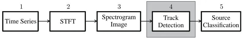
1 2 3 4 5
Time Series STFT SpectrogramImage Track Detection
[image:25.595.140.536.92.155.2]Source Classification
Figure 1.1: Flow diagram of the passive sonar process.
1.1
The Passive Sonar Problem
Passive sonar is a form of sonar in which no energy is emitted from the detection apparatus [178].
Instead, the acoustic pressure surrounding a hydrophone (the transducer) is converted into an
elec-trical signal and analysed to reveal the presence of a source within the environment. Passive sonar is typically used by navies for the identification of submarines, torpedoes and ships and within
science and ecology for the monitoring of marine mammals and fish. Currently, trained operators
analyse the passive sonar data in spectrogram images to detect and classify any acoustic sources in the surrounding environment [120]. This is a complex task, with many spectrograms being
analy-sed from an increasing number of look-directions, in which the detection of each track is critical to
subsequent information processing. Recent advances in mechanical technology, leading to noise reduction, has fuelled the need for more robust, reliable and sensitive algorithms to detect ever
quieter engines in real time and in short time frames. Also, recent awareness and care for
endange-red marine wildlife [125, 172] has resulted in increased data collection, which requires automated algorithms to detect calls and determine local specie population and numbers. Consequently, it is
of interest to develop computational algorithms to achieve track detection automatically.
The acoustic data observed via passive sonar systems is conventionally transformed from the
time domain into the frequency domain using the short-term Fourier transform [179]. This al-lows for the construction of a spectrogram image which provides a visual representation of the
distribution of acoustic energy across frequencies and over time [174]. The vertical axis of a
spec-trogram typically represents time, the horizontal axis represents the discrete frequency steps, and the amount of power observed by the hydrophone is represented as the intensity at each
time-frequency point. It follows from this that if a source which emits narrowband energy is present
during some consecutive time frames a track, or line, will be present within the spectrogram.
The process by which passive sonar exploits narrowband sound radiated in an underwater environment is outlined in Fig. 1.1. Passive sonar systems do not emit any sound and therefore
only sound radiated from the target can be detected by the receiver (box 1). The short-term Fourier
transform of the observed signal is calculated (box 2) to determine the power present at each frequency band in a particular time sample. These Fourier transforms are then collected together
and a spectrogram image is formed (box 3) which represents the energy at each time-frequency
point (these points will be discussed further, and illustrated, in the next section).
Sound sources such as ships and other machines radiate some of their energy as narrowband
tracks in a spectrogram that vary in frequency according to the state which the machine is in. For example, when a source is running at a constant speed and there is an absence of the Doppler
effect [49], the frequencies emitted are stationary and the narrowband energy that is radiated
re-sults in time-invariant tracks. Moreover, a source in which the machinery speed increases, i.e., the source is accelerating, results in tracks that increase in frequency over time. Other sources
of radiated narrowband sound that are not dependent on engine speed, the hydrodynamic flow
noise and the remainder of the machinery noise, result in constant frequencies regardless of the machine’s state. As each type of source emits a particular frequency pattern, it may provide
suf-ficient information for its identification using a spectrogram (Fig. 1.1, box 5). Urick presents a full discussion on the radiation of acoustic energy from submerged machinery in “Principles of
Underwater Sound” [174]. Due to the Doppler effect and the nature of the source’s machinery
the track is often time-variant and therefore, general line detection algorithms, as will be shown in this thesis, are not suitable. It still holds, however, that a particular, relative, frequency pattern
will be emitted by each source.
The principle source of complexity in the analysis of passive sonar is that all noise from each concomitant event in the underwater environment is observed. This results in the presence of large
amounts of non-uniform background broadband noise in the spectrogram. This noise distorts
the tracks, causing them to be broken, particularly at low frequency ranges, and also introduces points of high energy at spurious frequencies. Discriminating these from the signals of interest is
particularly hard in low signal-to-noise ratio conditions. Another cause for broken tracks in the
spectrogram is the Lloyd mirror, or image-interference, effect [174]. This occurs when the sea is calm; an interference pattern is created by constructive and destructive interference between the
direct and surface-reflected sound.
1.2
Data
Following the discussion of the problem, a detailed description of the type of signals that are under
consideration will be presented. Consequently, this provides a basis by which synthetic data can
be generated for evaluating algorithms designed to detect such signals.
1.2.1 Signal Generation
A continuous signalx(t), observed by a sensor, is the superposition of a longitudinal sound wave emitted by a sources(t), after propagation through, in this case, the ocean environments′(t)[174], and background noisen(t)[72], such that
x(t) =s′(t) +n(t). (1.1)
The detection of the periodic or near-periodic narrowband frequency components ofs′(t)through spectrogram analysis is the concern of this thesis. Periodicity is defined such that
whereP is the period of the signal, and near-periodicity such that
|s(t)−s(t+P)|< ε (1.3)
whereεis a marginal error resulting from a variation in periodicity. The effects of propagation will be discussed in more detail in Section 1.2.2. Throughout this thesis the noisen(t)is assumed to be Gaussian [72, 11].
The signal x(t)is sampled at a period ofTsseconds (a sampling rate offs ,1/TsHz) using
the Dirac comb [47] defined by
∆Ts(t),
∞
X
m=−∞
δ(t+mTs)
whereδis the Dirac delta, to form a discrete signalxs(t), such that
xs(t) =x(t)∆Ts(t). (1.4)
The periodTs(or sampling ratefs) is chosen according to the Nyquist sampling theorem such that the highest meaningful frequency in the application is representable.
This thesis concentrates on the detection of narrowband mechanical sources such as torpedoes,
ships and submarines within the ocean. Being mechanical devices, powered by an engine and
propelled by a propeller blades, the sound waves emitted are periodic [174]. As suchs(t), which is the superposition of a set of harmonically related sinusoids, comprises a fundamental frequency,
ω0t, being the lowest frequency sinusoidal in the sum, andhharmonics of this [11], such that
s(t) =µ+ h
X
k=1
Aksin(kω0tt+φ) (1.5)
whereωt
0 is the fundamental frequency at timetand, φ, its phase, his the number of harmonics observed,µis the mean value, andAkis the amplitude of thekth harmonic. These harmonics are
directly related to the rotational speed of the drive shaft.
Several other components of a mechanical device cause the emission of frequency components which are related to this fundamental frequency but which are not harmonics, i.e. they are not
integer multiples of the fundamental frequency, and these are referred to as inter-harmonics [115].
Reduction gear ratios connecting the propeller blades, the propeller blades themselves and the power plant emit additional low frequency inter-harmonic components [174]. Auxiliary units such
as pumps, generators, servos, and relays also emit noise in the ultrasonic region [139]. These,
the fundamental, harmonic and inter-harmonic, frequency components comprise the signature of a particular mechanical device [174]. The signature, due to the differences in the mechanical
construction and components, is unique for each type of device and will be referred to as the
pattern set,Ps, such that
where m1 = 1 and the term h ≥ 1 is the number of relative frequency components (the first component of the set corresponds to the fundamental frequency) of the signals(t).
The signals(t) can now be defined to be the superposition of sinusoids having harmonically related frequency components defined inPs, such that
s(t) =µ+ X mk∈Ps
Aksin(mkωt0t+φ) (1.6)
wheremk ∈Psis thekth relative frequency component ofPsandAkis its amplitude.
1.2.2 Signal Propagation
Physical phenomena may influence the signal so that the observed signal has different properties
from that which is emitted by the source. The passive sonar equation [173]
SL−TL=NL−DI+DT (1.7)
describes the effects of the oceanic environment upon the intensity of the signal and the conditions
upon which it is detectable against background noise. It has three fundamental parts, which are
all expressed in decibels (dB): the observed signal intensity, the noise levelN L, and the system’s detection threshold DT. The observed signal intensity is the difference between the radiated signal levelSL, in decibels, and the transmission lossTL, due to the signal’s propagation through the ocean. This occurs due to a combination of the following physical effects: spreading, ray path bending, absorption, reflection, and scattering. Therefore, the intensity level of the signal arriving
at the sensor is described by the left side of Eq. (1.7), that isSL−TL. In addition to receiving the source signal the passive SONAR sensor also receives ambient noiseNL. To some extent this can be counterbalanced by the gain of the receiver arrayDI [174], resulting in an overall noise level of NL−DI. When the equality in Eq. (1.7) holds the target is on the system’s detection threshold i.e. “a binary choice detector will dither between ‘target present’ and ‘target absent’
indications” [171].
The difference between the intensity of the observed source signals′(t) and that emitted by the sources(t), Eq. (1.1), can be expressed as a scaling of the emitted signal [189], such that
s′(t) =αs(t) (1.8)
whereαis the scaling factor, that isα∝SL−TL, and represents propagation loss.
In addition to this, when a source is performing a circling manoeuvre offset from the receiver,
is approaching the sensor, or is receding from the sensor, the Doppler effect [49] causes the emitted sound wave to compress or expand and therefore the perceived frequencyωˆt
0, may differ from that at the sourceω0t[66], such that
ˆ
ω0t = ( c c±vs)ω
t
0 (1.9)
upon the speed of sound in seawater and in 1981 a simplified, nine-term equation for calculating this speed,c(ms−1), was developed by Mackenzie [119], such that
c = 1448.96 + 4.591T −5.304×10⁻²T2+ 2.374×10⁻⁴T3+
1.340(S−35) + 1.630×10⁻²D+ 1.675×10⁻⁷D2−
1.025×10⁻²T(S−35)−7.139×10⁻¹³T D3 (1.10)
whereT is the temperature in degrees Celsius,S is the salinity in parts per thousand, andDis the depth in meters. Its ranges of validity are: temperature −2to30◦C, salinity30to40‰, and
depth 0 to8,000m. Nevertheless, if these conditions are unknown, or an approximate value is sufficient, c can be assumed to be 1,500ms−1 [139]. Other, more complicated, equations exist and are accurate over a wider range of conditions [53, 62], including the international standard
(UNESCO) algorithm [39, 186].
Taking the effect of amplitude scaling, by a factor ofα, and the changes in perceived frequency
ˆ
ω0tdescribed by the Doppler effect into account, Eq. 1.6, which previously described the observed signals′(t), can be re-written such that
s′(t) =µ+α X mk∈Ps
Aksin(mkωˆ0tt+φ). (1.11)
Using these properties, synthetic acoustic signals can be generated which mimic the behaviour of
a mechanical device operating in various states.
1.2.3 Spectrogram Formation
A spectrogramSis formed by splitting a discrete time-domain signalxs(t)into sectionsτseconds in length [101], such that
xms (t),xs(t+mR), t= 0,1, . . . , T −1
wherexm
s is themth frame of the signal,T =⌊τ fs⌋is the frame length (fsis the sample rate used
when sampling the continuous signal in Eq. 1.4) andT ≥1, andRis the time advance from one frame to the next (in number of samples). Throughout this thesisτ is taken to be one second and
Ris taken to beR=T /2, so that there is a half second overlap between each frame.
The power spectrum of a frame can be calculated using the Short-Term Fourier Transform
(STFT) [160], such that
Fm(ω) = T−1
X
t=0
xms (t)w(t)e−2πiωt, 0< ω < 2
T (1.12)
Frequency (Hz) P o w er (V 2 / H z )
200 300 400 500 600 700 800 900
0.0 0.5 1.0 1.5 2.0 2.5 3.0
Figure 1.2: Magnitude Squared of the Fourier transform of an acoustic signal at one time frame. The x-axis represents frequency (Hz) and the y-axis power (V2/Hz). The signal has frequency components of120, 240, 360, 480 and 600Hz plus noise derived from a Gaussian distribution (with mean SNR of3dB).
window function [76], such that
w(t) = 0.53836−0.46164 cos
2πt T −1
. (1.13)
The use of windows such as the Hamming window reduces the effects of ‘spectral-leakage’ [76], which occurs when processing finite-duration signals, by weighting the signal at the frame
boun-daries close to zero.
The STFT results in the magnitude and phase over frequency of the signal. By taking its squared magnitude and multiplying by a normalisation factor, the periodogram estimate of the
power spectrum is derived which satisfies Parseval’s theorem [146], according to
Pm(ω) = PT−11 t=0 |w(t)|2
|Fm(ω)|2. (1.14)
An example of the power spectrum of one time frame of a signal is presented in Fig. 1.2. It can be
observed that, at low SNRs, the components of the frequency-set indicated are indistinguishable from the noise. As such, the detection of low SNR frequency components is difficult in single time
frame STFTs. Nevertheless, over time, noise is uncorrelated and therefore has a relatively large
variance, however, a signal that contains a frequency component is correlated and therefore has less variance; under these assumptions the detection of the frequency components should be easier
within a number of successive power spectra.
Treating the power spectrum of a frame,[Pm(ω0)Pm(ω1) . . . Pm(ωN−1)], as a row vector, successive vectors can be stacked up and interpreted as a grey scale imageS, a spectrogram, which hasM rows andN columns, such that
S = [sij]M×N =
P0(ω0) P0(ω1) . . . P0(ωN−1)
P1(ω0) P1(ω1) . . . P1(ωN−1)
P2(ω0) P2(ω1) . . . P2(ωN−1)
..
. ... . .. ...
PM−1(ω0) PM−1(ω1) . . . PM−1(ωN−1)
T
im
e
(s
)
Frequency (Hz)
50 100 150 200 250 300 350
20 40 60 80 100 120
Figure 1.3: A spectrogram image where intensity represents signal power (voltage-squared per unit bandwidth, that is V2/Hz). In this example the tracks have an SNR of (from left to right): three3dB, three6dB, and three9dB.
wherei= 0,1, . . . , M −1is the time frame,j = 0,1, . . . , N−1is the frequency bin,N ∈ N
is the number of frequency bins calculated using the STFT, andM ∈Nis the number of previous
frames to be retained. Therefore, the grey scale intensity in a spectrogram represents the amount of energy present in each frequency component at a particular time frame. An example of a
spectrogram image, the composition of (M = 40) power spectra can be seen in Fig. 1.3. As each new power spectrum becomes available it is prepended onto the first row of the spectrogram and the oldest spectrum is removed, forming a “rolling window”, also known as a “waterfall display”.
A frequency component ofx(t), which is constant or varying slowly over time, and is therefore present in more than one consecutive row of S, is referred to as a track. A track appears in a spectrogram as a (perceptually) connected non-linear structure that can vary in its frequency
position in each time frame according to the state of the underlying mechanism. Several states have been mentioned with regards to the domain signals: constant, increasing, sinusoidal and
random. For example, a mechanical source that is constantly approaching then receding from the
receiver will emit a frequency component that undulates around a central frequency due to the Doppler effect. Within a spectrogram this is represented as a track that is sinusoidal in appearance.
Three examples of synthetic spectrogram images which represent a number of track appearances
are presented in Fig. 1.4.
As discussed previously, each of the components ofPswill form a track in the spectrogram
at a position relative to the fundamental frequency. For example an acoustic signal may contain fundamental frequencies and their harmonics and inter-harmonics at relative positions to them,
in spectroscopy analysis molecules with particular spectral characteristics could form the pattern
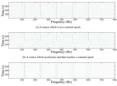
Frequency (Hz) T im e (s )
100 200 300 400 500 600 700 800
100 200 300
(a) A source which is at a constant speed.
Frequency (Hz) T im e (s )
100 200 300 400 500 600 700 800
100 200 300
(b) A source which accelerates and then reaches a constant speed.
Frequency (Hz) T im e (s )
100 200 300 400 500 600 700 800
100 200 300
[image:32.595.77.463.87.372.2](c) A source that repeatedly approaches and recedes from the receiver.
Figure 1.4: Three examples of synthetic spectrogram images which exhibit a variety of track appearances at an mean SNR of16dB. Intensity is proportional to power in voltage-squared per unit bandwidth, that is V2/Hz.
Within this thesis the mean, frequency domain, signal-to-noise ratio of a spectrogram is
calcu-lated such that [72]
SNR= 10 log10
¯ Pt ¯ Pb (1.16) ¯ Pt= 1
|Pt|
X
(i,j)∈Pt
sij, P¯b= 1
|Pb|
X
(i,j)∈Pb
sij (1.17)
wherePt={(i, j)|sij belongs to a track}is the set of points related to the frequency components ofs′(t)such thatP
t 6=∅andPb = {(i, j)|(i, j) ∈/ Pt}is the set of points which represent noise
such thatPb 6=∅.
There are two specific approaches to measuring the SNR in this problem and it is necessary to make the distinction: in the time domain (also known as the broadband SNR) or in the frequency
domain. As this thesis is concerned with the detection of tracks within a spectrogram image
the time domain SNR is not a true representation of the problem complexity, and therefore, all SNRs presented in this thesis are taken within the frequency domain according to Eq. 1.16. As
1.3
Thesis Contributions
Thesis proposition: to demonstrate that a multiple active contour framework is
ef-fective at detecting patterns of tracks in spectrograms.
The work is initiated with a full review of the algorithms that have been applied to the problem; this forms the first key contribution of this thesis. The review reveals that two areas have drawn
the majority of interest, statistical models, such as the hidden Markov model [150], and image
processing/pattern recognition. It is also concluded that, although there has been a great expansion of the areas of pattern recognition and image processing in recent years, there has been relatively
little research on applying these advances to the passive sonar domain. Additionally, many of
the machine learning techniques that are commonly known in the area of pattern recognition, and that may offer improvements over techniques already applied to the problem of spectrogram track
detection have not been evaluated. The active contour algorithm is found to encompass many of
the features that have been proposed for use in the detection of spectrogram tracks and to overcome some of the limitations of existing algorithms.
This motivates the next stage of research, and consequently the thesis’ second contribution:
an investigation into, and evaluation of, low-level pattern recognition and image processing tech-niques applied to the spectrogram track detection problem. This investigation involves the
defini-tion and evaluadefini-tion of an exhaustive detecdefini-tion method based on multi-scale template correladefini-tion
to demonstrate an ‘optimal’ detector’s performance. This is the thesis’ third contribution as it establishes a benchmark result, which is obtainable using all the information available to detect
low-level features. This feature detector is empirically compared with other ‘optimal’ detectors
that utilise less information, and also to feature detectors which utilise dimensionality reduction to simplify the detection process. One of which employs an equivalent data model to the
‘opti-mal’ detector and this comparison demonstrates that dimensionality reduction degrades detection performance. All of these low-level feature detectors are evaluated by calculating their Receiver
Operating Characteristic (ROC) curves on a set of spectrograms, which contain a variety of SNRs
and track appearances. It is shown that none of the standard feature detection methods reach the performance of the exhaustive detector. Nevertheless, near ‘optimal’ performance can be gained
by using machine learning techniques to extract filters from training data and fitting a statistical
model to classify unseen examples—simplifying the detector’s search space.
The findings and conclusions of this research motivate the development of a high-level track
detection framework using an active contour model. This incorporates an interchangeable
low-level feature detector into a single and multiple track detection algorithm—the thesis’ fourth contri-bution. The framework provides a flexible detection mechanism that allows for the detection of
tracks that have unknown appearances. Furthermore, this framework enables the enhancement of
detection probabilities by integrating information taken from either harmonically related positions in the spectrogram or from positions defined by the signature of a specific source. This is a
fur-ther contribution of this thesis. The framework is evaluated upon a set of synthetic spectrogram
for real-world data, allowing for accurate evaluations to be conducted. The measure used to eva-luate the track detection framework is the line location accuracy score [145], which has previously
been used by Di Martino and Tabbone [57] for evaluating algorithms applied to this problem. It
is shown through a number of empirical comparisons that the solutions presented in this thesis are necessary for the application of the active contour algorithm to this problem. Moreover, the
propo-sed active contour algorithm encompasses aspects of existing approaches, whilst overcoming some
of their limitations, such as: high computational complexity, sensitivity to noise, and assumptions of track structure, to name but a few. Ultimately, the algorithm is demonstrated to be an effective
method for the detection of tracks that display a variety structures.
1.4
Thesis Structure
The remainder of this thesis is organised as follows. In Chapter 2 a taxonomy, evaluation and
review of the spectrogram track detection algorithms found in the literature are presented. The evaluation criteria are defined and example applications are presented along with the criteria which
should be met to allow for the successful application of an algorithm. Due to the complexity of
quantitatively evaluating each algorithm upon a common data set, the methods are qualitatively evaluated based upon results and algorithm descriptions presented in the respective papers.
Chap-ter 3 presents an investigation into existing and novel low-level feature detection algorithms from
the areas of pattern recognition and image analysis. Also, an investigation into the detection of features in harmonically related positions is presented with the aim of enhancing feature
detec-tion in low SNR condidetec-tions. Chapter 4 proposes a high-level track detecdetec-tion framework for single
and multiple tracks which integrates the findings of the previous chapters into the active contour model. The chapter also contains an analysis of the computational complexity of the model. In
Chapter 5 the proposed track detection framework is evaluated and a discussion of its
The Field as it Stands
This chapter presents a review of the spectrogram track detection algorithms present in the
li-terature. Constructing such a review reveals the approaches that have been taken to solve this
problem whilst ascertaining their limitations, strengths and weaknesses—laying the foundations for future innovations within the field. The research surveyed here is taken from a variety of
computer science disciplines and is concerned with the specific problem of track detection
wi-thin spectrogram images applied to passive sonar. Whilst there is a huge amount of literature on acoustic analysis and pattern recognition the intersection of these fields is relatively small—this
chapter provides a review of this intersection. The algorithms are grouped within a taxonomy and
evaluated according to the following factors, some or all of which are essential for a successful application: their ability to cope with noise variation over time; high variability in track shape;
closely separated tracks; multiple tracks; the birth/death of tracks; low signal-to-noise ratios; their
ability to perform track association; that they have no a priori assumption of track shape; and, for real time implementations, that they are computationally inexpensive. This evaluation is based on
what is presented in the literature.
The chapter starts by defining the evaluation criteria. A taxonomy of the reviewed algorithms
is presented and these algorithms are surveyed and reviewed. This leads to a discussion of their principal shortfalls with respect to the criteria defined, and to the identification of issues to be
addressed in future research. Finally, the chapter’s summary is drawn.
2.1
Definition of Evaluation Criteria
The criteria by which the algorithms will be evaluated, some or all of which are essential for a
successful application, are defined below (in no particular order):
C1 Low SNR — Is reliable detection achieved in a frequency domain SNR below3dB, defined
as Eq. (1.16)?
C2 Temporal Noise Variability — Does the method allow for a time-variant noise model?
C3 Birth/Death of Tracks — Does the algorithm cope with the initiation and/or termination of tracks at some point within the spectrogram?
Application Typical Track Characteristics Criteria Required
Whale vocalisation Short duration, high variability, C2 Temporal Noise Variability, predictable appearance, initiation C3 Birth/Death Tracks, and termination observed. C4 Multiple Tracks,
C7 High Track Variability.
Passive Sonar Long duration, low SNR, initiation C1 Low SNR,
and termination observed. C2 Temporal Noise Variability, -Submarine Low variability. C3 Birth/Death Tracks,
C4 Multiple Tracks, C5 Closely Spaced Tracks, C6 Crossing Tracks, C7 High Track Variability, -Torpedo High variability. C8 No A Priori Shape Assumption.
Directly instrumented Long duration, high SNR. C4 Multiple Tracks, vibration analysis C5 Closely Spaced Tracks,
C6 Crossing Tracks, C7 High Track Variability, C8 No a priori Shape Assumption.
Table 2.1: Track characteristics and criteria specific to typical applications of spectrogram track detection algorithms.
C4 Multiple Tracks — Can the algorithm detect two or more separate tracks that exist concur-rently (in the same time frame)?
C5 Closely Spaced Tracks — Can the algorithm distinguish two or more tracks that are separa-ted by one frequency bin?
C6 Crossing Tracks — Will the algorithm detect and distinguish between multiple tracks that occupy the same point in a spectrogram for one or more consecutive time frames?
C7 High Track Variability — Does the algorithm detect time-invariant tracks that have high variability?
C8 No A Priori Shape Assumption — Is the method free from the assumption of a strict track
shape model and therefore can generalise to unknown cases?
C9 Track Association — Does the method output a series of points that it deems as belonging
to the same track?
C10 Computationally Inexpensive — Does the algorithm have an on-line computational burden
with less than polynomial complexity (not including any training requirements)?
The importance of each criterion depends upon the algorithm’s application, as each
applica-tion is concerned with the detecapplica-tion of signals with different characteristics. The dominant signal
characteristics of some example applications, along with the criteria that should be met to demons-trate an algorithm’s suitability, are identified in Table 2.1. In addition to these, the need to fulfil the
C9 (Track Association) criterion is dependent upon the type of subsequent processing that will be
2.2
Algorithm Taxonomy
Algorithms presented in the literature are identified and categorised in Table 2.2 (in chronological order within subheadings). It should be noted that the majority of research has been conducted in
the areas of statistical modelling, image processing and neural networks, with additional
contri-butions from relaxation techniques. Hidden Markov models have attracted, by far, the largest proportion of research interest. Considering the relative size, breadth of techniques and the recent
speed of progress in the areas of image processing and pattern recognition they have received very
little attention in the literature.
It should be noted for completeness that additional methods exist, particularly those that are presented in the literature as Master’s theses [197, 40], which it was not possible to survey
(al-though they have been included in the taxonomy presented here). Nevertheless, it is believed that similar techniques from different authors have been reviewed and therefore that the key algorithms
are still presented in this review.
2.3
Literature Survey
This section presents a review of the methods found in the literature under the categories presented
in Table 2.2. The techniques presented here are specifically those found in the literature that have been applied to the problem of spectrogram track detection in passive sonar systems. As such this
is not intended to form a full catalogue of general purpose detection or tracking methods as this
falls outside the problem domain specified by this thesis.
It was noted in Section 1.2.3 that there are two distinct approaches to measuring the SNR in spectrogram images. In order to convert between the two, full information regarding the
short-term Fourier transform process is needed and this is not obtainable for all of the papers reviewed
in this survey. Therefore, where time domain signal-to-noise ratios are presented the distinction is noted.
2.3.1 Maximum Likelihood Estimators
Maximum likelihood estimators (MLE) are based upon statistical assumptions regarding the data
in question. A statistical test is defined that decides whether a frequency bin contains noise or
a track (signal). Maximum likelihood methods make detections on single spectrogram points and lend themselves to the detection of temporally invariant tracks as no assumptions are made
regarding the temporal evolution of a track. Nevertheless, the simplicity of the detection methods
limit their application to high SNR cases. This limitation is overcome with MLE methods based on convolution, which make assumptions regarding the temporal evolution of a track to augment
low SNR detection. The large search space needed to perform real world detections, however,
makes them unfeasible.
Approach Representative Works Maximum Likelihood
MLE Maximum value [152] Correlation [8] Multi harmonic [20]
Image Processing Techniques
Likelihood Ratio Test Morphological operators [3]
Hough Transform Graph theoretic tracking & heuristic search Hough transforma[30] Multi-stage Decision Multi-stage decision cost function optimisation [55]
Steerable Filter Gap bridging, region locating & multi-stage decision process [56, 57] Two-Pass Split-Window Broadband subtraction via estimation [38]
Edge Detector Gaussian filtered spectrogram [69]
Neural Networks
Supervised Learning Autoassociative memory & multi-layer perceptron [99] Multi-layer perceptron [114]
Multi-layer perceptron constrained using Ockham’s networks [98] MNET1 [4]
MNET2 [4] RNET [4]
Unsupervised Learning Kohonen self-organising map [54]
Statistical Models
Dynamic Programming Logarithmic likelihood function [162] Hidden Markov Model Viterbi & max amplitude [169]
Viterbi, “mixed” track & threshold [190] Viterbi & “mixed” track [191] Viterbi & double threshold [165]
Viterbi & probabilistic data association [88] Parallel, multi model detection [175]
Forward-backward linking, SNR estimate & track gradient [137] Forward-backward linking & SNR estimate [138]
Viterbi & SNR estimate [138]
Forward-backward linking & spectrum interpolation [74]
Tracking Algorithms
Particle Filter Formant detection [163]
Relaxation Methods
Relaxation Relaxationa[197]
Simulated Annealing Simulated annealinga[40]
Simulated annealing [112]
Expert Systems
Double detection Double threshold & priority ranking [117]
a
[image:38.595.55.486.186.621.2]Master’s theses which are not surveyed in Section 2.3.
frequency position in the observation,ωiˆ , that is,
ˆ
ωj = arg max i |
sji|, j= 0,1, . . . , M−1. (2.1)
This is repeated for each observation. Thus, a single frequency is detected within each and every
time framej, and the estimated track is a series of these frequency positions. Ferguson [66] has applied this method to the analysis of aircraft acoustics received by an underwater hydrophone.
According to Barrett and McMahon [20], the single frequency case described above, Eq. (2.1),
can be extended to the detection of a single frequency that exhibits harmonics, such that
ˆ
ωj = arg max i
m
X
l=1
|sj,li|2, j= 0,1, . . . , M −1. (2.2)
These early MLE techniques disregard information describing the distribution of the inten-sity values attributed to each class, opting to use the maximum instead. This would lead to the
method mistaking spurious high power noise for instances of a track. Nevertheless, an important
introduction in the multi-harmonic case is the concept of detecting a fundamental frequency by in-tegrating information from its harmonics. This integration of information should greatly increase
the detectability of tracks at low SNRs.
Altes [8] presents a likelihood ratio test based upon the correlation of a spectrogram with an expected, noise free, reference spectrogramZk= [zji(ρk)], such that
p(S|Zk)≈
M−1
X
j=0
N−1
X
i=0
−zji(ρk)
σ2 +
sjizji(ρk) σ4
(2.3)
where σ is the standard deviation of the time domain noise, which is assumed to be known a
priori. This process is repeated for K reference signal hypotheses (each with a hypothesised signal parameter ofρk) and the maximum response is taken to be the detected signal, such that
ˆ
k= arg max
1≤k≤K
[lnp(S|Zk)].
The use of the correlation function allows for the detection of very weak SNR tracks.
Never-theless, for the method’s use in remote sensing applications, where the state and behaviour of the
phenomenon under observation are unknown, a very large reference set is needed. For example, performing a full search for instances of the sinusoidal track model outlined in Section 3.3.1,
which has five free parameters (the additional parameters are the frequency position and phase
of the sinusoidal track), would result in a search complexity of O(n5)and this complexity grows exponentially with each additional parameter.
2.3.2 Image Processing
Image analysis is a vast research area, and provides a wide range of techniques that could be beneficial to this problem. These are often inspired by human visual perception models, which
suggests they might be applicable to this problem, as it is accomplished by human operators. The
complexity of more advanced methods, however, often makes real-time implementation difficult.
2.3.2.1 Two-Pass Split-Window
Chen et al. [38] propose the use of the two-pass split-window (TPSW) to estimate the background
broadband noise within a spectrogram. Once an estimate of this has been calculated, subtracting it from the image should result in a cleaned spectrogram containing narrowband tracks. The TPSW
algorithm consists of two steps: first a local mean is calculated over a neighbourhood surrounding
each bin in the STFT, such that
ˆ
sji= 1 2W + 1
i+W
X
l=i−W
sjl, i=W, . . . , N −1−W (2.4)
wherej= 0,1, . . . , M−1and2W+ 1is the number of bins used to calculate the local mean. The result,ˆsji, is clipped and a second, local, mean is calculated upon these (as defined by Eq. (2.4)).
Although this is a filtering technique, a threshold criterion can be defined upon the TPSW output and a detection made using this. As with any filtering technique, there is a balance to
be made between the amount of smoothing and the detectability at low SNRs. In this case, this is
controlled with the window sizeW. As the TPSW is calculated independently for each time step in the spectrogram it has no assumption of track structure. This allows the detection of time-invariant
tracks that may be highly irregular in appearance.
2.3.2.2 Edge Detection
Gillespie [69], proposes an edge detection method that initially smoothes the spectrogram using a
Gaussian filterG, such that
S′ =S∗G (2.5)
G=
1 2 1 2 4 2 1 2 1
. (2.6)
The benefit of smoothing is that it prevents edges from breaking up into many parts; the detrimental
effect is a reduction of the spectrogram’s resolution if the smoothing kernel is too large.
Each point(i, j)in the smoothed spectrogram S′ is thresholded by comparison to the back-ground measurement bji. This background measurement is continuously updated to allow for
time-invariant noise conditions and computed independently for each frequency bin, such that
bji =bj,i−1+
s′
ji−bj,i−1 α