Output frequency response function-based analysis for nonlinear Volterra systems

promoting access to White Rose research papers

White Rose Research Online

Universities of Leeds, Sheffield and York

http://eprints.whiterose.ac.uk/

This is an author produced version of a paper published in Mechanical Systems and Signal Processing.

White Rose Research Online URL for this paper: http://eprints.whiterose.ac.uk/3554/

Published paper

Jing, X.J., Lang, Z.Q. and Billings, S.A. (2008) Output frequency response

function-based analysis for nonlinear Volterra systems, Mechanical Systems and Signal Processing, Volume 22 (1), 102 - 120.

Output Frequency Response Function based Analysis for

Nonlinear Volterra Systems

Xing-Jian Jing*, Zi-Qiang Lang, and Stephen A. Billings

Department of Automatic Control and Systems Engineering, University of Sheffield Mappin Street, Sheffield, S1 3JD, U.K.

{X.J.Jing, Z.Lang & S.Billings}@sheffield.ac.uk

Abstract

Analysis of nonlinear systems has been studied extensively. Based on some recently developed results, a new systematic approach to the analysis of nonlinear Volterra systems in the frequency domain is proposed in this paper, which provides a novel insight into the frequency domain analysis and design of nonlinear systems subject to a general input instead of only specific harmonic inputs using input-output experimental data. A general procedure to conduct an output frequency response function (OFRF) based analysis is given, and some fundamental results and techniques are established for this purpose. A case study for the analysis of a circuit system is provided to illustrate this new frequency domain method.

Keywords

Output frequency response function, Nonlinear systems, Volterra series

1 Introduction

Frequency domain analysis of a linear system can usually provide some intuitional insights into the system of interest, and thus is extensively used in engineering analysis and design. However, when it comes to a nonlinear system, it is not as easy as that for a linear system to perform a frequency domain analysis. The frequency domain theory for linear systems can not directly be extended to the nonlinear case. It is also known that nonlinear systems are often observed to have harmonics, complex inter-modulations and even chaos

etc, which transfer energy between different frequencies and give outputs at some quite different frequencies to those of the input. These phenomena further complicate the study of nonlinear systems in the frequency domain. A systematic approach to the analysis of nonlinear systems in the frequency domain is yet to be developed.

by using its describing function (Taylor 1999, Graham and McRuer 1961). This method can only be used to analyse a specific nonlinear term subject to a harmonic input. Limitations of the describing function based analysis are noted in many cases (Engelberg 2002). To overcome the drawbacks of the describing functions, there are some improved methods reported in literature (Sanders 1993, Elizalde and Imregun 2006, Nuij et al 2006). Moreover, the frequency output properties of a class of nonlinear systems driven by multiharmonic signals are also studied by classifying nonlinear distortions into harmonic and interharmonic contributions (Solomou et al 2002). Alternatively, for a wide class of nonlinear systems, frequency domain analysis can also be conducted based on Volterra series theory (Volterra 1959, Rugh 1981). It has been proved in Sandberg (1982ab, 1983ab) and Boyd and Chua (1985) that there exists a locally convergent Volterra series expansion of finite order for any time invariant causal nonlinear systems under certain conditions. The nonlinear systems which have a Volterra series expansion are simply referred to as nonlinear Volterra systems. Based on the Volterra series expansion, the generalized frequency response function (GFRF) is proposed in George (1959). Thereafter, many researches on the frequency domain analysis of nonlinear Volterra systems are carried out by using this concept (Brilliant 1958, Kim and Powers 1988, Bendat 1990, Nam and Powers 1994, Petkovska and Do 2000). This kind of frequency domain analysis methods can deal with nonlinear systems driven by a general input and does not necessarily restrict to a specific nonlinear term, thus is a more general methodology. However, it is noted that estimation and computation of the GFRFs and Volterra kernels for a nonlinear Volterra system usually involve too much complicated computation and symbolic operations (Yue et al. 2005). This, to a certain extent, inhibits the understanding and application of the corresponding results. It can be seen that a straightforward analytical expression for the relationship between system time-domain model parameters and system output frequency response can considerably facilitate the analysis and design of nonlinear systems in the frequency domain.

based analysis, allows analysis, design and optimization of output frequency response of nonlinear Volterra systems to be conducted in terms of system time domain model parameters, and has no restriction on input signal. A general procedure is proposed for the new frequency domain analysis method, and some fundamental results and practical techniques are developed to support the application of this new method. A case study is provided to illustrate the effectiveness of the new results.

2 Fundamental concept of the OFRF based analysis for nonlinear systems

Nonlinear systems considered in this paper can be described by the following nonlinear differential equation (NDE) model

0 ) ( ) ( ) , , (

1 0 , 0 1 1

1 , 1 =

∑∑ ∑

∏

∏

= = = + + = = + + M m m p K k k q p p i k k p i k k q p q p q p i i i i dt t u d dt t y d k k

c L (1)

where () ()

0 t x dt t x d k k k = =

, p+q=m,

∑

∑

∑

= = = + + ⋅ ⋅ = ⋅ K k K k K k

k, pq 0 0 pq 0

) ( ) ( ) ( 1 1

L , M is the maximum degree of

nonlinearity in terms of y(t) and u(t), and K is the maximum order of the derivative. In this model, the parameters such as c0,1(.) and c1,0(.) are linear parameters, which correspond to

the linear terms in the model, i.e., k _k

dt t y

d ()

and k _k

dt t u

d ()

for k=0,1,…,L, and cpq(⋅) for p+q>1 are

nonlinear parameters corresponding to nonlinear terms in the model of the form

∏

∏

+ + = = q p p i k k p i k k i i i i dt t u d dt t y d 1 1 ) ( )

( _{, e.g., y(t)}p_u(t)q_{. p+q is called the nonlinear degree of the nonlinear}

parameterc_pq(⋅). Moreover, c_pq(⋅)and cp'q'(⋅)are referred to as different type of nonlinearity if

'

p

p≠ or q≠q'. Similar to the NDE model (1), a discrete nonlinear model known as NARX

model is often used for practical nonlinear system identification from experimental data, which is given by

∑ ∑

∏

∏

∑

= = + + = = + = + − − = m p K k k q p p i i p i i q p q p M

m pq

k t u k t y k k c t y

0 , 1 1 1

1 , 1 1 ) ( ) ( ) , , ( )

( _L (2)

In engineering practise, the NDE or NARX model can represent a wide class of nonlinear dynamical systems and include several well known nonlinear input-output models as special cases (Chen and Billings 1989).

∫

∫

∞ ∞ − ∞ ∞ − − + +

= _{n n n n n}

n

n j j h j d d

H ( ω1,L, ω ) L (τ1,L,τ )exp( (ω1τ1 L ω τ )) τ1L τ (3)

wherehn(τ1,L,τn)is a real valued function of τ1,L,τn called the nth order Volterra kernel of

the system. By probing method (Rugh 1981), the recursive algorithms for the computation of the GFRFs for model (1) and (2) were developed in Peyton-Jones and Billings (1991) and Billings and Peyton-Jones (1989). Based on these results, the system output frequency response can be obtained for a general input signal as (Lang and Billings 1996)

∫

∏

∑

= + + = − = = = ω ω ω ω σ ω ω ω π ω ω ω n n i i n n n n N n n d j U j j H n j Y j Y j Y L L 1 1 1 1 1 ) ( ) , , ( ) 2 ( 1 ) ( ) ( ) ( ) 4 ( ) 4 ( b a

where U(jω)is the Fourier transform of a general input u(t), and N is the largest order of the

Volterra series expansion. When the system is subject to a multi-tone input described by

∑

= ∠ + = K i i i

i t F

F t u 1 ) cos( )

( ω (5)

then the system output spectrum can be written as

∑

∑

= + + = = = ω ω ω ω ω ω ω ω ω ω n k k n n k k

k k n n n N n n F F j j H j Y j Y j Y L L L 1 1

1, , ) ( ) ( ) ( 2 1 ) ( ) ( ) ( 1 ) 6 ( ) 6 ( b a

where

{

}

⎪⎩ ⎪ ⎨ ⎧ ∈ =± ± = ∠ else 0 , , 1 , if )

( F e k K

F k

F j

i i ω ω L

ω .

Although these results provide an important basis for frequency domain analysis of nonlinear systems, it can be seen that the direct computation of system output spectrum involves very complicated integral and symbolic operations in multi-dimensional complex space, and the analytical relationship between model parameters and output spectrum can not be demonstrated clearly by the recursive algorithms. For these reasons, the concept of output frequency response function (OFRF) was proposed in Lang et al (2006), which defines an analytical relationship between the system output spectrum and the model parameters of nonlinear systems, and reveals that the system output spectrum of model (1) can be written into a simple polynomial form as

∑

= N s N s N N s j j j s j j

j x x

j Y L L L 1 1 1 ( ) 1 )

( ω γ ω (7)

where x1Lxs_N are the elements in a set consisting of all the system nonlinear parameters,

N

s j

j_1L are nonnegative integers, andγ ₁ (ω)

N s

j

jL represents the coefficient of the term N

s N

j s

j _x

x1_L

which is a function of frequency variable and depends on the system linear parameters. The OFRF was further studied in Jing et al (2006a) through parametric characteristic analysis. The results explicitly reveal the analytical polynomial relationship between system nonlinear parameters and system output spectrum, and allow the detailed structure of the OFRF to be determined up to any high orders without complicated symbolic computations in multi-dimensional complex space. Based on the results in Jing et al (2006a,b), Equation (7) can be written into a more explicit form as

∑

= ⋅ ⋅ = N n T n n j H CE j Y 1 ) ( )) ( ( )

( ω ϕ ω (8a)

where, ϕn(jω)stands for a complex valued function vector which has the same dimension as

)) ( (H_n ⋅

CE , CE(.) is a novel coefficient extraction operator defined in Jing et al (2006a,b) (for

the detail refer to Appendix A), and CE(Hn(⋅))is the parametric characteristics of the n

th-order GFRF H_n(⋅), which can be recursively determined by

⎣ ⎦ ) 8 ( )) ( ( )) ( ( )) , , ( ( 1 0 , 2 1 2 0 , 1 , 1 1 1 , 0 1 b H CE C C H CE C C j j H CE p n p n p n p q n q p q n p n q n n n ⎟ ⎟ ⎠ ⎞ ⎜ ⎜ ⎝ ⎛ ⋅ ⊗ ⊕ ⊕ ⊕ ⎟ ⎠ ⎞ ⎜ ⎝ ⎛_{⊕⊕ ⊗ ⋅} ⊕ = _{− +} + = + − − − = − = ω ω _L

where _, [ _, (0, ,0), _, (0, ,1), , _, ( , , )]

43 42 1L L L L q p q p q p q p q

p c c c K K

C

+

= for some p, q. The terminating condition is

CE(H1(.))=1. Obviously, the elements of CE(Hn(⋅))are functions of the system time domain

model parameters which define nonlinearities. For more clarity, (8a) can be rewritten as

T j j

Y( ω)=ψ ⋅Φ( ω) (9)

where ( ()), ( )

[

1( ) 2( ) ( )

]

1 ω ϕ ω ϕ ω ϕ ω

ψ CE Hn j j j N j

N

n⊕ ⋅ Φ = L

=

= . Note that ϕ1(jω)=H1(jω) is the

first order GFRF, which represents the linear part of model (1) or (2).

Equation (8a) or (9) provide a straightforward analytical expression for the relationship between system time-domain model parameters and system output frequency response. Hence, it can considerably facilitate the analysis and design of nonlinear systems in the frequency domain, and provide a useful insight into the frequency domain analysis and design of nonlinear Volterra systems. In many practical applications, the problems are, how some specific model parameters affect system output spectrum, and what the effect is. Therefore, the main idea for the OFRF based analysis proposed in this paper is, once the model of a nonlinear system is given in the form of model (1) or (2), then CE(Hn(⋅))can be

computed according to (8b) and ϕn(jω)can be obtained according to a numerical method

specific input function can be achieved, which is an analytical function of nonlinear parameters of the nonlinear system model, and finally frequency domain analysis for the nonlinear system can be conducted in terms of the specific model nonlinear parameters of interest. Related to this topic, some useful techniques and fundamental results are developed in this study.

In what follows, Section 3 introduces a general procedure for the OFRF based analysis, and some useful techniques for the determination of OFRF are proposed such that the computation of the OFRF of a nonlinear Volterra system automatically by computer programming; further results for the OFRF based analysis are given in Section 4, which facilitates the determination of the parametric characteristics of the OFRF for some special cases and demonstrates some potential application of the OFRF based analysis; a case study is given in Section 5 to illustrate the effectiveness of these new results; finally, Section 6 summarizes the conclusions of this study.

3 A general procedure for the OFRF based analysis

Generally, given the system model (1) or (2), there are several basic steps for the OFRF based analysis. An assumption is made that the input-output relationship of the interested system has a convergent Volterra series expansion. Usually, there must be a locally convergent Volterra series expansion for a time invariant causal nonlinear system in the neighbourhood of its stable equilibrium for a sufficient small input according to the theories in Sandberg (1982ab, 1983ab) and Boyd and Chua (1985). Based on the system model, the following procedure and related techniques can be followed to obtain the OFRF of the nonlinear system of interest, and then frequency domain analysis and design of the nonlinear system can be carried out based on the system OFRF.

3.1 Computation of the parametric characteristics of OFRF

This step is to derive ( ())

1 ⋅

⊕ =

= n

N

n CE H

ψ in (9).

3.1.1 Determination of the largest order of the Volterra series expansion

To derive the parametric characteristics of OFRF, the first task is to compute the largest order, i.e., N, of the Volterra series expansion for the nonlinear system, which is basically determined by the significance of the truncation error in the Volterra series expansion of finite order. This can alternatively be to evaluate the magnitude value of the nth-order output frequency response Yn(jω) . For example, based on some new bound characteristics of

NARX model developed recently in Jing et al 2006c, the magnitude bound of Yn(jω)can be

T n n n

n j b

Y ( ω) ≤α ⋅ ⋅h (10)

where αn,hnare complex valued functions, and bnis a function vector of the system model

parameters. For the detailed definitions forαn,bn,hnrefer to Appendix B or Jing et al (2006c).

If the magnitude bound of a certain order of Yn(jω)is less than a predefined value (for

instance 10-8), then the largest order N is obtained. It should be noted that the magnitude bound is a function of the model nonlinear parameters, therefore, the largest ranges of interest for each nonlinear parameter should be considered in the evaluation of Yn(jω).

3.1.2 Determination of the parametric characteristics of the GFRFs

Once the largest order N is determined, the next step is to derive the parametric characteristics of GFRFs for the nonlinear system, i.e., CE(H_n(⋅))from n=2 to N, which will

be used in the computation of ( ())

1 ⋅

⊕ =

= n

N

n CE H

ψ . Note that CE(H_n(⋅)) is computed in terms of

the parameter vectors , [ , (0,L,0), , (0,L,1),L, , (_1L42, ₄,₃)]

q p q p q

p q

p q

p c c c K K

C

+

= for some p,q in (8b).

Basically, for some specific parameters to be analysed for a system, CE(Hn(⋅))can be

recursively computed by Equation (8b) with respect to these parameters of interest with the other nonzero nonlinear parameters being 1. Alternatively, CE(H_n(⋅)) can also be computed

for all the nonlinear parameters for system model (1) or (2), then the general form of

)) (

(H_n ⋅

CE needs only be computed once and can be stored for any future usage by replacing

the corresponding parameter vector Cp,q of interest with respect to the specific nonlinear

system, while the nonzero parameters of no interest being 1.

In order for CE(H_n(⋅)) to be determined directly without recursive computations, an

algorithm can be obtained by using the following result.

Proposition 1. The elements of CE(Hn(jω1,L,jωn)) includes the nonlinear parameter in

C0n and all the non-repetitive monomial functions of the nonlinear parameters in (1) or (2) of

the form Cpq ⊗Cp1q1 ⊗Cp2q2 ⊗L⊗Cp_kq_k, where the subscripts satisfy p q p q n k

k

i

i i+ = +

+

+

∑

=1

)

( ,

k n q

pi+ i≤ −

≤

2 , 0≤k≤n−2, 2≤ p+q≤n−k and 1≤ p≤n−k . That is, the set of all the

subscript combinations of the form (p,q,p1,q1Lpk,qk) corresponding to the nonlinear parameter monomials of the form Cpq⊗Cp1q1⊗Cp2q2 ⊗L⊗Cp_kq_k which are included in

⎪ ⎪ ⎭ ⎪⎪ ⎬ ⎫

⎪ ⎪ ⎩ ⎪⎪ ⎨ ⎧

− ≤ + ≤ − ≤ + ≤

+ = + +

+

− ≤ ≤ − ≤ ≤

∑

=

k n q p k n q p

k n q p q

p

k n p n

k

q p q p q p

i i k

i

i i k

k

2 , 2

) (

1 , 2 0

) , ,

, , (

1 1

1 L ∪(0,n) (11)

Proof. See Appendix C. 

Consider two subscript combinations (p,q,p1,q1,p2,q2) and (p,q,p2,q2,p1,q1) which

correspond to the nonlinear parameter monomials Cpq⊗Cp₁q₁ ⊗Cp₂q₂ and Cpq⊗Cp2q2 ⊗Cp1q1

respectively. Obviously, the two monomials are the same one. In this case the two subscript combinations are equivalent and regarded as to be repetitive with respect to each other, thus only one is counted in set (11). According to Proposition 1, if all the non-repetitive subscript combinations in (11) are determined, then the nonlinear parameter monomials involved in

)) (

(H_n ⋅

CE can be obtained directly. Computation of, for example, CE

(

H4(jω1,L,jω4)

)

is given

to illustrate the result in Proposition 1:

When k=0, all the subscript combinations are (p,q): (0,4); (1,3), (2,2),(3,1),(4,0). Hence, the involved nonlinear parameters are: C0,4, C1,3, C3,1, C2,2, C4,0;

When k=1, then p+q+p1+q1=4+1=5, all the non-repetitive subscript combinations are

(p,q,p1,q1): (1,1,0,3), (1,1,1,2), (1,1,2,1), (1,1,3,0),

(1,2,0,2), (1,2,2,0), (2,0,0,3), (2,0,2,1), (2,0,3,0), (2,1,0,2), (3,0,0,2) Hence, the involved nonlinear parameter monomials are:

C1,1⊗C0,3, C1,1⊗C1,2, C1,1⊗C2,1, C1,1⊗C3,0, C1,2⊗C0,2, C1,2⊗C2,0, C2,0⊗C0,3, C2,0⊗C2,1,

C2,0⊗C3,0, C2,1⊗C0,2, C3,0⊗C0,2

When k=2, then p+q+p1+q1+p2+q2 =4+2=6 , all the non-repetitive subscript

combinations are

(p,q,p1,q1,p2,q2): (1,1,0,2,0,2), (1,1,0,2,1,1), (1,1,0,2,2,0), (1,1,1,1,1,1), (1,1,1,1,2,0),

(1,1,2,0,2,0), (2,0,0,2,0,2), (2,0,0,2,2,0), (2,0,2,0,2,0) Hence, the involved nonlinear parameter monomials are:

C1,1⊗C0,2⊗C0,2, C1,1⊗C0,2⊗C1,1, C1,1⊗C0,2⊗C2,0, C1,1⊗C1,1⊗C1,1, C1,1⊗C1,1⊗C2,0,

C1,1⊗C2,0⊗C2,0, C2,0⊗C0,2⊗C0,2, C2,0⊗C0,2⊗C2,0, C2,0⊗C2,0⊗C2,0

Therefore,

(

H4(jω1, ,jω4)

)

CE L = C0,4+C1,3+C3,1+C2,2+C4,0+C1,1_oC0,3+C1,1_oC1,2+ C1,1_oC2,1

+C1,1_oC3,0+C1,2_oC0,2+C1,2_oC2,0+C2,0_oC0,3+ C2,0_oC2,1+

+C2,0_oC3,0+ C2,1_oC0,2+C3,0_oC0,2+ C1,1_oC0,22+C1,12_oC0,2

where“⊕” and “⊗” are substituted by “+” and “o” for clarity, respectively.

Simply, the computation of the parametric characteristic CE(Hn(⋅))can be conducted as

follows, which is referred to as Process A. For0≤k≤n−2,

(1) Generate all the combinations (r0, r1, r2…, rk) satisfying r r n k

k

i

i = +

+

∑

=1

0 and

k n

ri ≤ −

≤

2 with respect to a specific value of k;

(2) Generate all the possible combinations (pi,qi) with respect to each ri satisfying pi+qi =

ri, and note that when it is for r0, 1≤ p0≤n−k;

(3) All the possible combinations can now be generated based on Step (1) and (2), then remove all the repetitive terms;

(4) CE(H_n(⋅)) is obtained in terms of the parameter vectors Cp,qfor some p,q, which can

be stored for any future usage. For a specific nonlinear system, CE(Hn(⋅))can be obtained

only by replacing the corresponding interested parameter vector Cp,qwith respect to the specific nonlinear system, and the other parameters in CE(H_n(⋅)) are set to be zero if it is

zero or 1 if it is not of interest to be analysed.

(5) Achieve the final result by manipulating CE(H_n(⋅)) according to the operation rules of

“⊕” and “⊗” (See Appendix A), and removing the repetitive terms.

By this method, the parametric characteristic CE(H_n(⋅))can be obtained without recursive

computations.

For a summary, the parametric characteristic vector ( ())

1 ⋅

⊕ =

= n

N

n CE H

ψ can be computed by

following the process bellow, which is referred to as Process B:

(1) Determine the set of the nonlinear parameters of interest, denoted by SC;

(2) Determine the largest possible ranges for the interested nonlinear parameters, denoted by∂SC;

(3) Determine the largest order N of the Volterra series expansion according to (10) and the discussions following inequality (10).

(4) Computation of CE(Hn(⋅)) with respect to the interested parameters SC following

Process A or Equation (8b) from n=2 to N.

(5) Combine the final parametric characteristic vector ( ())

1 ⋅

⊕ =

= n

N

n CE H

ψ .

Based on the results in the previous steps, this step is mainly to determine

[

( ) ( ) ( )

]

)

(jω = ϕ1 jω ϕ2 jω L ϕN jω

Φ in (9), then the OFRF in (9) is obtained consequently.

Since the system model is known and the parametric characteristic vector

)) ( ( 1 ⋅ ⊕ = = n N

n CE H

ψ is achieved, the complex valued function vector Φ(jω)can be derived with

respect to any a specific input by following a numerical method used in Lang et al 2006.

Note that Φ(jω)is invariant with respect to ( ())

1 ⋅

⊕ =

= n

N

n CE H

ψ , therefore, Φ(jω)can be derived

as follows, which is referred to as Process C:

(1) Choose a series of different values of the interested nonlinear parameters which are properly distributed in ∂SC, and thus form a series of vectors ψ1Lψρ, whereρ is a

positive integer number, such that

⎪⎩ ⎪ ⎨ ⎧ ≠ ≠ Ψ Ψ = ≠ Ψ ψ ρ ψ ρ 0 ) det( 0 ) det(

T (12)

where _[ T T_]T

1 ψρ

ψ _L

=

Ψ , det(.) is the determinant of matrix (.), and ψ denotes the

dimension of vector ψ .

(2) Choose an observed frequency point ω where the output frequency response of the nonlinear system is to be analysed or designed. Usually, the harmonic frequency with the largest output magnitude is a proper observed frequency point.

(3) Actuate the system using the same input under the different values of the nonlinear parameters ψ1Lψρ , then collect the time domain output y(t) for each case, and

consequently obtain a series of output frequency response Y(jω)1LY(jω)ρ at the

frequency ω by FFT technique. (4) Step 3 yields

) ( : ) ( ) ( ) ( ) ( ) ( ) ( ) ( 2 1 2 1 2 1 ω ω ω ω ω ϕ ω ϕ ω ϕ ψ ψ ψ ω ρ ρ j YY j Y j Y j Y j j j

j T ₌

⎥ ⎥ ⎥ ⎥ ⎥ ⎦ ⎤ ⎢ ⎢ ⎢ ⎢ ⎢ ⎣ ⎡ = ⎥ ⎥ ⎥ ⎥ ⎦ ⎤ ⎢ ⎢ ⎢ ⎢ ⎣ ⎡ ⋅ ⎥ ⎥ ⎥ ⎥ ⎥ ⎦ ⎤ ⎢ ⎢ ⎢ ⎢ ⎢ ⎣ ⎡ = Φ ⋅ Ψ M M M l (13)

Hence, (_l=ψ )

⎪⎩ ⎪ ⎨ ⎧ ≠ ⋅ Ψ Ψ Ψ = ⋅ Ψ = Φ ₋ − ψ ρ ω ψ ρ ω ω ) ( ) ( ) ( ) ( ₁ 1 j YY j YY

j T _{T T (14)}

should be noted that there may be some other methods for this purpose such as Least mean square, Recursive Least Square, and OLS etc, which are not discussed in detail here.

Based on the results above, the OFRF (9) is now completely determined by following Step 3.1 and 3.2 for the nonlinear system of interest subject to a general input. Moreover, note that since CE(H_n(⋅))is known, andΦ(jω)=

[

ϕ1(jω) ϕ2(jω) L ϕN(jω)

]

is determined,

then T

n n

n j CE H j

Y ( ω)= ( (⋅))⋅ϕ ( ω) is also determined, which represents the analytical function for the nth-order output frequency response (in (4b) or (6b)) of nonlinear systems.

3.3 Analysis based on the OFRF

The OFRF of nonlinear systems defined in (9) which can be obtained by following the procedure above is an explicit analytical function of the system time domain model parameters of interest. Based on this expression, analysis, design and optimization of nonlinear Volterra systems described by model (1) or (2) can be carried out in terms of these interested model parameters which define system nonlinearities and may represent some structural and controllable factors of a practical engineering system. For example, the sensitivity of system output frequency response with respect to a nonlinear parameter can be studied based on the analytical expression (9). And also, by using the link between the nonlinear terms of interest and the components of a practical engineering system and structure, the OFRF may provide a useful insight into the design of nonlinear components in the system to achieve a desired output performance. It should be noted that the control input of nonlinear systems is not necessarily harmonic input. Therefore, the OFRF based analysis method provides a novel and more general approach to the analysis and synthesis of a considerably wide class of nonlinear systems in the frequency domain. These are further discussed in detail in the following section.

4 Some further results for the OFRF based analysis

The parametric characteristic vector CE(Hn(⋅))for all the nonlinear model parameters can be obtained according to (8b) or Process A, and if there are only some parameters of interest, the computation can be conducted by only replacing the other nonzero parameters with 1 as mentioned above. Note that in many cases, only several special nonlinear parameters of the same degree and the same type, for example some parameters in Cp,q, are of interest for a specific nonlinear system. Then the computation of the parametric characteristic vector in (9) can be simplified greatly. The following results are established for this purpose.

⎥ ⎥ ⎦ ⎤ ⎢ ⎢ ⎣ ⎡ = ⎥⎦− ⋅ − ⎥ ⎢ ⎣ ⎢ − + − ) ( ) ( 1 1 2

1, , )) 1

(

( p q p posn q

n

n

n j j c c c

H

CE ω _L ω _L δ (15)

where _⎣⎦⋅ is to get the integer part of (.),

⎩ ⎨ ⎧ = = else 0 0 if 1 )

(p p

δ , and

⎩ ⎨ ⎧ > = else 0 0 if 1 )

(x x

pos .

Proof. See Appendix D. 

Note that here c may be one parameter or a vector of some parameters of the same nonlinear degree and type in Cpq. Also note that _{1 L4243}

n

n _{c c c}

c = ⊗ ⊗ and ⊗ is the reduced

Kronecker product defined in Appendix A, when c is a vector. Proposition 2 establishes a very useful result to study the effects on the output frequency response from a specific nonlinear degree and type of nonlinear parameters. It should be noted that if some nonlinear parameters in model (1) or (2) are zero, only part terms inCE(Hn(jω1,L,jωn)) take an

effective role. The detailed form of CE(Hn(jω1,L,jωn))can be derived from Process A and B.

However, direct using equation (15) does not affect the final result and is more convenient.

Corollary 1. If all the other degree and type of nonlinear parameters are zero except that

Cp,q=c is nonzero. Then the parametric characteristic vector of the nth-order GFRF with respect to the parameter c is: if (n>p+q and p>0), or (n=p+q), and if additionally 1₁

− +

−

q p

n _{is an}

integer, then

1 1

1, , ))

(

( + −

−

= p q n

n

n j j c

H

CE ω L ω

else CE(Hn(jω1,L,jωn))=0

which can be summarized as

(

1 ( ) ( )

)

1 1 1 1 )) , , ( ( 1 1

1 _{p q} p posn q

n q p n c j j H

CE p q

n

n

n ⎟⎟⋅ − −

⎠ ⎞ ⎜ ⎜ ⎝ ⎛ ⎥ ⎦ ⎥ ⎢ ⎣ ⎢ − + − − − + − ⋅ = +− − δ δ ω

ω _L (16)

Proof. The results are directly followed from Propositions 1 and 2. 

Corollary 1 provides a more special case of nonlinear system (1) or (2). There are only several nonlinear parameters of the same nonlinear type and degree in the considered system. This result will be used in the example of Section 5. Based on the results above, the following results can be achieved for the output frequency response.

Corollary 2. Consider only the nonlinear parameter Cp,q=c. The parametric characteristic vector of the output spectrum in (9) with respect to the parameter c can be written as

⎥ ⎥ ⎦ ⎤ ⎢ ⎢ ⎣ ⎡ = ⋅ ⊕ = = ⎥⎦− ⋅ − ⎥ ⎢ ⎣ ⎢ − + − = ) ( ) ( 1 1 2

1 ( ()) 1

)) (

( p q p posN q

N

n N

n CE H c c c

j Y

CE ω δ

If all the other degree and type of nonlinear parameters are zero except that Cp,q=c is nonzero (p+q>1). Then the parametric characteristic vector of the output spectrum in (9) with respect to the parameter c is:

if p=0

[

1 (1 ( ))

]

))

( 1 ( )) ( ( 1 )) (

(Y j CE H posq N c posq N

CE = ⊕ q ⋅ ⋅ − − = ⋅ − −

= ω

ψ

else

⎥ ⎥ ⎦ ⎤ ⎢

⎢ ⎣ ⎡ = ⋅ ⊕

=

= ⎢⎣⎢ − +−⎥⎦⎥

+ − + ⎥⎦

⎥ ⎢⎣ ⎢

− + −

=

1 1 2

1 ) 1 ( 1 1

0 ( ()) 1

)) (

( N pq

i q p q

p N

i CE H c c c

j Y

CE ω _L

ψ 

Proof. The results are straightforward from Proposition 2 and Corollary 1. 

The results above involve the computation of cn. If c is an I-dimension vector, there will be many repetitive terms involved in cn. To simplify the computation, the following lemma can be used.

Lemma 1. Let be c=[c1,c2,…,cI] which can also be denoted by c[1:I], and _{1 L4243}

n

n _{c c c}

c = ⊗ ⊗ ,

“⊗” is the reduced Kronecker product defined in Appendix A, n≥1and I≥1. Then

[

n n n n n i n n I

]

n _{c c c s si s c c s c}

c = − ⋅ _{, ,} −1_{[ (1)} − ₍₎ +_{1: (1) ]}⋅ _{, ,} −1_{[ (1) ]}⋅

1 1

L L

where

∑

= −

= I

i j

n

n s j

i

s() ( ) 1, s(.)1=1, and 1≤i≤I. Moreover, ( )= (1)n+1

n _s

c

DIM , and the location of

cin in cn is s(1)n+1-s(i)n+1+1. Proof. See Appendix E. 

Based on the result in Corollary 2 and equation (9), with respect to a specific parameter c, the output frequency response function can be written as

L L+ l l + +

+ +

= ( ) ( ) ( ) ( )

)

(jω ϕ0 jω cϕ1 jω c2ϕ2 jω c ϕ jω

Y (17a)

Since Y(jω)is also a function of c, therefore, (20a) is rewritten more clearly as

L L+ l l + +

+ +

= ( ) ( ) ( ) ( )

) ;

(jω c ϕ0 jω cϕ1 jω c2ϕ2 jω c ϕ jω

Y (17a)

) ;

(j c

Y ω is in fact a series of an infinite order. When it is for a finite order N, the right side of

equation (17) stops at lwhich is a positive integer and can be determined by Corollary 2.

)

( ω

ϕi j can be obtained by following the same method as Process C. If all the other degree

and type of nonlinear parameters are zero except that Cp,q=c is nonzero (p+q>1), thenϕi+1(jω)=ϕi(jω)(the later is defined in equations (8-9)), Based on equation (17), the

(1) Optimization of the output frequency response in terms of nonlinear parameters.

This is to give a desired output frequency response _Y*(_jω)_{, an optimal c}* _{can be found}

such that ) ( ) ; (

min_{Y jω c Y}* _jω

c −

Many methods in literature for optimization can be adopted for this purpose, which are not discussed here.

(2) Sensitivity of the output frequency response to nonlinear parameters.

Based on equation (17), this can be obtained easily as

L l

L+ l l + +

+ =

∂

∂ ( ; ) _{( ) 2 ( )} −1 _{( )}

2

1 ω ϕ ω ϕ ω

ϕ ω j c j c j c c j

Y ₍₁₈₎

Similarly, the sensitivity of the magnitude of the output frequency response with respect to the nonlinear parameters can also be derived. Note that

) ) ( ) ( ) ( )( ) ( ) ( ) ( ( ) ; ( ) ; ( ) ; ( 2 2 1 0 2 2 1 0 2 L

L − + − + − +

+ + + = − = ω ϕ ω ϕ ω ϕ ω ϕ ω ϕ ω ϕ ω ω ω j c j c j j c j c j c j Y c j Y c j Y

_L l _{l L}

l

l l l

l _{= + + + + +}

⎟ ⎟ ⎟ ⎠ ⎞ ⎜ ⎜ ⎜ ⎝ ⎛ ℜ + =

∑

∞

∑

= = + ≤ ≤≤≤− 2 2 2 2 1 0 1 ,1 0 0

0, 2c ( , ) : p cp c p c p

j i j i i j i ϕ ϕ ϕ

ϕ (19)

where ℜ(⋅)is to get the real part of (.), and <x,y> is the inner product of x and y. It is obvious

that the spectral density of the output frequency response is still a polynomial function of the parameter c. Note that equation (19) can also be directly derived by following Process C. Thus, the sensitivity of the magnitude of the output spectrum to the parameter c can be obtained as

∑

∞

∑

= = + ≤ ≤≤≤− − ⎟ ⎟ ⎟ ⎠ ⎞ ⎜ ⎜ ⎜ ⎝ ⎛ ℜ = ∂ ∂ = ∂ ∂ 1 ,1 0 1 2 ) , ( 2 ) ; ( 2 1 ) ; ( ) ; ( 2 1 ) ; ( l l l l l l j i j i i j i c c j Y c c j Y c j Y c c j Y ϕ ϕ ω ω ω ω (20a)

Given (18), (20) can also be computed as

) ) ; ( ) ; ( ) ; ( ( ) ; ( ) ; ( ) ; ( ) ; ( ) ; ( 2 1 ) ; ( ) ; ( 2 1 ) ; ( 2 c j Y c j Y c c j Y c c j Y c j Y c j Y c c j Y c j Y c c j Y c j Y c c j Y ω ω ω ω ω ω ω ω ω ω ω − ⋅ ∂ ∂ ℜ = ⎟ ⎠ ⎞ ⎜ ⎝ ⎛ ∂ − ∂ + − ∂ ∂ = ∂ ∂ = ∂ ∂ (20b)

practice, the oscillation in system output should be suppressed as small as possible. Based on

equation (20), it can be seen that it should be ( ; ) <0

∂ ∂

c c j

Y ω

for some c in order to reduce the

magnitude level of output frequency response by properly designing the value of c. Consider equation (19), the following conclusion is obvious.

(a) ( ; ) <0

∂ ∂

c c j

Y ω

for some c some 0, ( ( ), ( ) ( ) ) 0

,1 0

1 _{> <}

< ℜ > ∃

⇒

∑

= + ≤ ≤≤≤ −

−

n j i n j i i n

j n

i j signc j

n ϕ ω ϕ ω

(b) p1=ℜ(<ϕ0(jω),ϕ1(jω)>)<0⇒there exists ε>0 such that 0

) ; (

< ∂ ∂

c c j

Y ω

for 0<c<ε or

0

< <

−ε c . Where,

⎩ ⎨ ⎧ −

≥ =

else 1

0 1

)

(x x

sign .

If a nonlinear parameter c satisfies p1=ℜ(<ϕ0(jω),ϕ1(jω)>)<0, then it can be utilized for

the purpose of output oscillation suppression.

(3) Evaluation of the radius of convergence for the output frequency response with respect to nonlinear parameters.

It is followed from (17) that the radius of convergence is given by

) (

) (

lim 1

ω ϕ

ω ϕ

j j R

l l l

− ∞ →

= (21)

Obviously, if |c|<R, then the series is convergent. Define a Ratio Function

c c

j j c

R

) (

) ( ) ;

( 1

ω ϕ

ω ϕ

l l

l = − (22)

which is a function of l and also varying with different nonlinear parameters. It can be seen that, if

l l l

l

Δ Δ > Δ

ΔR( ;c1) R( ;c2) ₍₂₃₎

then the output spectrum has a larger radius of convergence with respect to c1 than that with

respect to c2. Equation (22) and inequality (23) can be used as an evaluation of the effect on

the system stability from a specific parameter and the comparative advantage between different parameters. This analysis can provide some useful information for the design of system output frequency response in terms of model parameters.

There may be some other results can be developed based on equation (17) and (19). This is under study and will be discussed in the future. And it should also be noted that similar results can be established when there are multiple type and degree of nonlinear parameters of interest simultaneously.

[image:17.595.196.400.120.235.2]

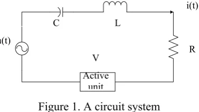
To demonstrate the effectiveness and application of the new OFRF based analysis method, a simple circuit system is studied in this section, which is shown in Fig 1.

Figure 1. A circuit system

There are two nonlinear components and one active unit in this circuit. The output property

of the capacitor satisfies = 1(

∫

i(t)dt+C1

(

∫

i(t)dt

)

3)

C

U , and the resistor (() ()3)

1i t

R t i R

U = + . In

this study, the active unit is designed to satisfyU =c1i(t)2

∫

i(t)dt+c2i(t)

(

∫

i(t)dt

)

2. The system

dynamics can be described by

( )

)

( 1 )

( 1 3

3

1 − =

∫

+

∫

+ −

− idt C idt

C V i R i R dt di L

u (24a)

For convenience, let the output be

∫

=D i t dt

y () (24b)

The task for this case study is to investigate how the nonlinear terms included both in passive and active unites affect the output and what the effect might be, and thus to provide a useful analysis for the design of corresponding nonlinear parameters to achieve a desired output frequency response.

For clarity in discussion, let x=

∫

idt, c3 =C1 C, c4 =R⋅R1,L=240, C=1/16000, R=296,

and D=16000, then (24) can be rewritten as

) ( 296

16000

240 3

4 3 3 2 2 2

1x x c xx c x c x u t

c x x

x&&=− − &− & − & − − & + (25a)

y=16000x (25b)

(25a) is a simple case of the NDE model (1) with M=3, K=2, c10(2)=240, c10(1)=296,

16000 )

0 (

10 =

C , c30(111)=c4, c30(110)=c1, c30(100)=c2, c30(000)=c3, c01(0)=−1, and all the other

parameters are zero. Therefore, what is interested in for this study is to analyse the effect of the nonlinear terms with coefficients c1, c2, c3 and c4 on the system output frequency

response. This may provide a useful insight into the nonlinear parameter design for a predefined output performance in the frequency domain. To achieve this objective, the procedure proposed in Section 3 are adopted to derive the OFRF of system (25), and the results in Section 4 will be used for the computation of the parametric characteristic of the

Active unit

V

C L

R u(t)

OFRF with respect to the nonlinear parameters c1, c2, c3 and c4. Moreover, though the

method proposed in this paper is suitable for a general input function u(t), yet for convenience in discussion, the input of system (25) is considered to be a sinusoidal function

) 1 . 8 sin( 100 )

(t t

u = . In the following, the procedure proposed in Section 3 is followed to

conduct an OFRF based analysis. To illustrate the new results more clearly and conveniently, the parameter c2 under the case of c1=c3=c4=0 is studied firstly in detail.

(1) Determine the parametric characteristics of OFRF

Note that all the interested nonlinear parameters belong to C30, and the other degrees of

nonlinear parameters are all zero. Thus Corollary 1 and 2 can be utilised directly. Therefore,

(

)

_⎟⎟ ⎠ ⎞ ⎜⎜ ⎝ ⎛ ⎥⎦ ⎥ ⎢⎣ ⎢ − − − ⋅ = − ⋅ ⎟⎟ ⎠ ⎞ ⎜⎜ ⎝ ⎛ ⎥⎦ ⎥ ⎢⎣ ⎢ − − − ⋅ = − − 2 1 2 1 ) ( ) 3 ( 1 2 1 2 1 )) , , ( ( 2 1 2 1 1 n n c n pos n n c j j H CE n n n

n ω L ω δ δ δ

⎣ ⎦ ⎥⎦ ⎤ ⎢⎣ ⎡ = ⎥ ⎥ ⎦ ⎤ ⎢ ⎢ ⎣ ⎡ = ⋅ ⊕ = = − ⎥⎦ ⎥ ⎢⎣ ⎢ − + − + − + ⎥⎦ ⎥ ⎢⎣ ⎢ − + − = 2 1 2 1 1 2 1 ) 1 ( 1 1 0 1 1 )) ( ( )) ( ( N q p N i q p q p N i c c c c c c H CE j Y CE L L ω ψ

where c=c2. To derive the detailed form for ψ , the largest order N should be determined first

according to Process B in Section 3.2. In order to have a larger range in which the

parameters can vary, in this case let (0,108)

2∈

c . Then the magnitude bound ofYn(jω)can be

evaluated as mentioned in Process B. However, for paper limitation, the detailed computation is omitted in this case. Simply, the largest N can be set to be a proper value after several trails. It can be verified that N=23 is enough for use in this case. Therefore,

⎣ ⎦

⎥⎦ ⎤ ⎢⎣

⎡

= _{1 c c}2 _c23−12

L

ψ =[1, c2, c22, c23, c24, c25, …, c211]

(2) Determination of the complex valued function Φ(jω) for OFRF

Following Process C, the matrix _[ T T_]T

1 ψρ

ψ _L

=

Ψ should be constructed first. Note that in

many cases, the parameters may be set to be very large values and cover a very large range. This will make the element values in the matrix Ψ extraordinarily large. Then when the inverse of matrix Ψ is computed, there may be some computation error involved in Matlab. To overcome this problem, ψ in (18b) can be rewritten as

⎣ ⎦ ⎣ ⎦ ⎥⎦ ⎤ ⎢⎣ ⎡ = ⋅ ⊕ = + − + − − ⎥⎦ ⎥ ⎢⎣ ⎢ − + − = 2 1 2 1 2 2 1 ) 1 ( 1 1

0 ( ())/ 1 ( / ) ( / ) ( / )

N N i q p q p N

i kCE H k k c k k c k L k c k

ψ

Then equation (9) can be rewritten as

[

][

]

T

T _{c k c k c k j k j k j}

j c

j

where_l=

⎣

N−1₂

⎦

_{. Moreover, the range for each parameter can be divided into several}

sub-range, and the final result is the combination of these results obtained for each sub-range. In

this case, let k=105, then 2 [0,1000]

2 =c _k ∈

c . Choose c2 to be the following values,

respectively, for the simulation study to construct T T T

]

[ψ1 Lψρ

=

Ψ , i.e.,

0.1,1,50,65,80,100,150,200,250,300,350,400,450,500,550,600,650,700,750,800,850,900, 950,980,1000. The output frequency response

)

(jω

YY =

[

Y(jω)1 Y(jω)2 L Y(jω)ρ

]

of system (25) at ω=8.1rad/s corresponding to different values of c2 can be obtained through

FFT of the time-domain output response. Then using (26), it can be derived from (14) that

[

]

T

T _{j k j k j}

j ) ( ) ( ) ( ) ( ω = ϕ1 ω ϕ2 ω L lϕl ω

Φ = (_ΨT_Ψ)−1_ΨT_⋅YY(_jω) _{. Therefore, the output}

frequency response function of system (25) with respect to nonlinear parameter c2 in the case

of c1=c3=c4=0 is obtained as

Y(jω;c2)= (2.060893505718041e+002 -2.402014548824790e+002i)

+ k-1 ( -5.14248529981906 + 5.35676372314361i) c2

+ k-2 (0.08589533966805 - 0.08827649204263i) c22

+ k-3 (-8.068953639113292e-004 +8.248154776018186e-004i) c23

+ k-4 (4.598423724418538e-006 -4.686570228695798e-006i) c24

+ k-5 (-1.679591261850433e-008 +1.708497491564935e-008i) c25

+ k-6 (4.056287337706451e-011 -4.120496550333245e-011i) c26

+ k-7 (-6.544911009113156e-014 +6.641760366680977e-014i) c27

+ k-8 (6.976300614229155e-017 -7.073928662624432e-017i) c28

+ k-9 (-4.713366512185836e-020 +4.776287453573993e-020i) c29

+ k-10(1.827866445826756e-023 -1.851299290299388e-023i) c210

+ k-11(-3.098310700824303e-027 +3.136656793561425e-027i) c211

Based on this function, (19) can be further computed as

L L L+ l l+ +

+ +

= 2 ₂

2 2 1 0 2

) ;

(j c p cp c p c p

Y ω

Note that this is an alternating series and it holds that pi > pi+1 and pi →0. Hence the

series will keep decreasing when c is going larger and within its radius of convergence. By following the similar method demonstrated above, the output frequency response functions of system (25) with respect to nonlinear parameters c1, c2, c3 and c4 under any cases can all

be obtained, for instance Y(jω;c1) , Y(jω;c3) , and Y(jω;c4) with the other nonlinear

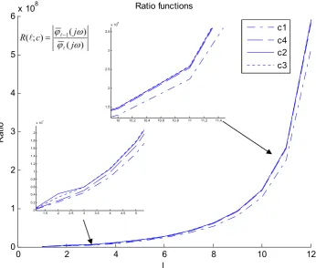
parameters zero if not appearing in the function. The results are shown in Figure 2-4.

Figure 2 shows that the variation of the magnitude of the output frequency response functions with respect to each nonlinear parameter. It can be seen that the larger the nonlinear terms are, the larger the effect they have on the system output frequency response is. However from both Figure 2 and Figure 3 it can also be seen that the system output frequency response is much more sensitive to the variation of the nonlinear parameters when they are small. Once the value of a nonlinear parameter is sufficient large, then the sensitivity will tend to be zero. Comparisons between these four nonlinear terms, it can be concluded that the system output frequency response is more sensitive to the variation of the nonlinear parameter c4 when the values are small; however when the values of each

nonlinear parameters are sufficient large, the system output spectrum is more sensitive to the nonlinear parameter c2. From Figure 4 it can be seen that the convergence of the output

frequency response functions are all very fast. This can also be understood that the energy disperse quickly with the nonlinear order going larger. It is noted that the ratio functions of c2 and c3 go up much faster than that of c1, especially c2. This implies that the system is more

robust with respect to c2 and the radius of convergence corresponding to c2 should be larger.

Simulation tests verify that the system is still stable when c2=1017 where the magnitude of

the output spectrum is 0.0216, while the system tends to be unstable when c1 tends to be

larger than 108.

From the analysis above for the four nonlinear parameters of nonlinear degree 3, respectively, it can be concluded that

(1) The system is more robust to the nonlinear parameters c2, c3 and c4, and less robust to c1;

(2) The system output spectrum is more sensitive to c4 and less sensitive to c3;

(3) If the output spectrum with respect to a nonlinear parameter is an alternating series satisfying pi > pi+1 and pi →0, then the system output spectrum may be reduced to

zero if additionally the radius of convergence for this parameter is sufficiently large; (4) Introduction of nonlinear terms into a linear system may greatly improve the

necessarily proportional to the increase of the values of the nonlinear parameters, and the stability of a nonlinear system is not necessarily deteriorated with the values of the nonlinear parameters increasing;

(5) Several simple nonlinear terms can work together to achieve a better performance.

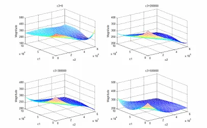
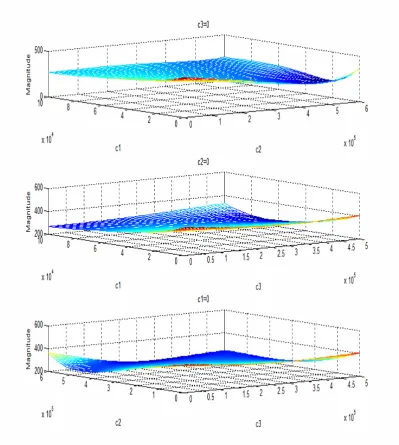
To demonstrate further the advantage of the OFRF based analysis and to show more clearly the effect on the system output spectrum from several nonlinear parameters together, the OFRF with respect to c1, c2 and c3, i.e., Y(jω;c1,c2,c3) is derived. Let

], 10 5 , 0 [ ], 10 6 , 0 [ ], 10 , 0

[ 5

3 5 2

5

1∈ c ∈ ⋅ c ∈ ⋅

c and c4=-500, then the largest order N of the output

spectrum can be determined to be 11 according to the evaluation of (10), and consequently (18b) can be obtained as (c=[c1,c2,c3])

⎣ ⎦

⎥⎦ ⎤ ⎢⎣

⎡

= _{1 c c}2 _c11−12

L

ψ =[1,c1,c2,c3,c12,c1c2,c1c3,c22,c2c3,c32,c13,c12c2,c12c3,c1c22,c1c2c3,

c23,c22c3,c2c32,c33,c14,c13c2,c13c3,c12c22,c12c2c3,c12c32,c1c23,c1c22c3,c1c2c32,c1c33,c24,c23c3,

c22c32,c2c33,c34,c15,c14c2,c14c3,c13c22,c13c2c3,c13c32,c12c23,c12c22c3,c12c2c32,c12c33,c1c24,

c1c23c3,c1c22c32,c1c2c33,c1c34,c25,c24c3,c23c32,c22c33,c2c34,c35].

Finally, following the same procedure, the OFRF Y(jω;c1,c2,c3)in this case can be obtained.

The results are shown in Figure 5-6. It can be seen that

(1) By using the OFRF, the output spectrum can be plotted and analyzed under different combinations of the nonlinear parameters c1, c2 and c3. This provides a straightforward

insight into the relationship between system output spectrum and model parameters which define nonlinearities.

(2) The OFRF is varying with different values of c1, c2 and c3. Thus the parameters

should be optimized in order to get the best output frequency response performance. The OFRF provides a useful basis for this kind of analysis and optimization.

From the discussions above, it can be concluded that the OFRF based analysis provides a novel, effective and useful approach to the analysis and design of nonlinear Volterra systems in the frequency domain.

6 Conclusions

some existing methods such as GFRF based analysis which is usually difficult to be used to obtain some quantitative information about a system, and involves too much recursive complicated computations which may even be difficult to be carried out when the involved nonlinearity order is too large, and describing function based methods which can only deal with harmonic input. Some fundamental results, techniques, and a general procedure for the determination and analysis of OFRF are provided to support the application of this novel frequency domain analysis method. A case study for a simple circuit system shows that the OFRF based analysis is a useful approach to the analysis, design and optimization of nonlinear Volterra systems in the frequency domain.

Acknowledgements

The authors gratefully acknowledge the support of the Engineering and Physical Science Research Council, UK and the EPSRC-Hutchison Whampoa Dorothy Hodgkin Postgraduate Award, for this work.

0 1 2 3 4 5 6 7 8 9

x 107 0

50 100 150 200 250 300 350

Nonlinear parameters c1,c2,c3 and c4

Ma

gn

itu

de

Output frequency response fuctions

c1

Simulation data c4

Simulation data c2

Simulation data c3

[image:22.595.93.457.387.688.2]

Simulation data

1 2 3 4 5 6 7 8 9 10 11 x 106 -15

-10 -5 0 5 10

Nonlinear parameters c1, c2 and c3

M

agn

itu

de of

t

he s

ens

iti

vi

ty

f

unc

tion

s (

10e

-5

)

Sensitivity of OFRF to nonlinear parameters

[image:23.595.98.452.78.374.2]

c1 c1 c2 c2 c3 c3

Fig. 2 Sensitivity function of the OFRFs with respect to c1 to c3 respectively

0 2 4 6 8 10 12

0 1 2 3 4 5 6x 10

8

l

Ra

tio

Ratio functions

c1 c4 c2 c3

Fig. 3 Ratio functions with respect to c1 to c4 respectively

1.5 2 2.5 3 3.5 4 4.5 5 0

0.2 0.4 0.6 0.8 1 1.2 1.4 1.6 1.8 2

x 107 10 10.2 10.4 10.6 10.8 11 11.2 11.4 1.5

2 2.5 3 3.5

x 108

c c j Y

∂ ∂ ( ω; )

c c j Y

∂ ∂ ( ω; )

) (

) ( ) ;

( 1

ω ϕ

ω ϕ

j j c

R

l l

[image:23.595.108.455.436.730.2]

[image:24.595.77.484.115.366.2]

[image:25.595.77.477.73.519.2]

Fig. 5 Output spectrums with respect to any two combinations of c1, c2 and c3

Appendices

Appendix A: Coefficient extraction (CE) operator (Jing et al 2006ab) Consider a series

σ σ f

c f

c f c

HCF = 1 1+ 2 2+L+ ∈Ψ

where the coefficients ci (i=1,…,σ ) are complex numbers, σ = C denotes the dimension of

with respect to the coefficients ci for i=1,…,σ . Define a Coefficient Extraction operator σ

C

→ Ψ

:

CE for this series such that

σ σ = ∈C

= c c c C

H

CE( CF) [ 1, 2,L, ]

where_Cσ_{is the σ-dimensional complex valued vector space. This operator has the following}

properties, also acting as operation rules: (1) Reduced vectorized sum “⊕”.

CE(HC1F1 +HC2F2)=CE(HC1F1)⊕CE(HC2F2)=C1⊕C2=[C1,C2′] , C2′ =VEC(C2 −C1∩C2) ,

where C1=

{

C1(i)1≤i≤ C1

}

,C2 =

{

C2(i)1≤i≤ C2

}

, VEC(.) is a vector consisting of all the

elements in set (.).C2′is a vector including all the elements in C2 except the same

elements as those in C1.

(2) Reduced Kronecker product “⊗”.

⎪⎭ ⎪ ⎬ ⎫

⎪⎩ ⎪ ⎨ ⎧

≤ ≤

= =

⊗ = ⊗

= ⋅

3

2 1 1 2 1 3 3 2

1

1

] ) ( , , ) 1 ( [ ) ( )

( ) ( )

( _{11 2 2 11 2 2}

C i

C C C C C C i C VEC C

C H

CE H

CE H

H

CE CF CF CF CF

L

which implies that there are no repetitive elements in C1⊗C2.

(3) Invariant. (a)CE(α⋅H_CF)=CE(H_CF) ∀α∈ℜbut is not a parameter of interest; (b)

C H

CE H

H

CE( CF1 + CF2)= ( C(F1+F2))=

(4) Unitary. If H_CFis not a function of ci for i=1…n, 1CE(H_CF)= .

When there is a unitary 1 in CE(HCF), there is a nonzero constant term in the corresponding series HCF which has no relation with the coefficients ci (for i=1…n). In addition, if H_CF=0, then CE(HCF)=0.

(5) Inverse. CE-1(C)=HCF.

(6) CE(HC₁F₁)≈CE(HC₂F₂) if the elements of C1 are the same as those of C2, where “≈” means equivalence, i.e., both series are in fact the same result considering the order of cifi in the series has no effect on the value of a function series HCF. This further implies that the CE operator is also commutative and associative, for instance,

1 2 2

1 ( )

)

(H ₁₁ H _{2 2} C C CE H _{2 2} H ₁₁ C C

CE CF + CF = ⊕ ≈ CF + CF = ⊕ . Hence, the results by the CE

operator with respect to the same purpose may be different but all correspond to the same function series and are thus equivalent.