Complex robot training tasks through bootstrapping system identification

This is a repository copy of

Complex robot training tasks through bootstrapping system

identification

.

White Rose Research Online URL for this paper:

http://eprints.whiterose.ac.uk/74638/

Monograph:

Akanyeti, O., Nehmzow, U. and Billings, S.A. (2008) Complex robot training tasks through

bootstrapping system identification. Research Report. ACSE Research Report no. 982 .

Automatic Control and Systems Engineering, University of Sheffield

[email protected] https://eprints.whiterose.ac.uk/

Reuse

Unless indicated otherwise, fulltext items are protected by copyright with all rights reserved. The copyright exception in section 29 of the Copyright, Designs and Patents Act 1988 allows the making of a single copy solely for the purpose of non-commercial research or private study within the limits of fair dealing. The publisher or other rights-holder may allow further reproduction and re-use of this version - refer to the White Rose Research Online record for this item. Where records identify the publisher as the copyright holder, users can verify any specific terms of use on the publisher’s website.

Takedown

If you consider content in White Rose Research Online to be in breach of UK law, please notify us by

Complex Robot Training Tasks through Bootstrapping

System

Identification

Otar Akanyeti

_{, Ulrich Nehmzow}

_{, and S A Billings}

1

Dept Computer Science, University of Essex

2

Dept Computer Science, University of Ulster, Ireland

Department of Automatic Control and Systems Engineering

The University of Sheffield, Sheffield, S1 3JD, UK

Research Report No. 982

Complex Robot Training Tasks through Bootstrapping System

Identification

Otar Akanyeti

, Ulrich Nehmzow

, and Steve Billings

Abstract— Many sensor-motor competences in mobile robotics applications exhibit complex, non-linear characteris-tics. Previous research has shown that polynomial NARMAX models can learn such complex tasks. However as the complex-ity of the task under investigation increases, representing the whole relationship in one single model using only raw sensory inputs would lead to large models. Training such models is extremely difficult, and, furthermore, obtained models often exhibit poor performances.

This paper presents a bootsrapping method of generating complex robot training tasks using simple NARMAX models. We model the desired task by combining predefined low level sensor motor controllers.

The viability of the proposed method is demonstrated by teaching aScitos G5_{autonomous robot to achieve complex route} learning tasks in the real world robotics experiments.

I. INTRODUCTION

One approach to generating controllers for robotics sensor-motor tasks, using non-linear mapping techniques, can be summarized as follows: The programmer demonstrates the desired behaviour to the robot by driving it manually in the target environment. During this run, the sensor pre-ception and the desired velocity commands of the robot are logged. Having thus obtained training data, the sensor based control models — which link the perception of the robot to the desired motor commands to achieve the de-sired task — are obtained using non-linear mapping tech-niques ([Demiris and Hayes, 1996] [Nehmzow et al., 2005], [Akanyeti et al., 2007a]) (see figure 1). Single model is usu-ally enough to identify the whole relationship successfully.

Desired Output Raw

Sensor

Perception Modelling Non−linear

Fig. 1. The general approach to generate controllers for sensor-motor tasks.

This approach has been extensively used by the mo-bile robotics community and some good results have been achieved in many different mobile robotics ap-plications ([Nguyen and Widrow, 1990], [Pomerleau, 1993], [Akanyeti et al., 2007b]). However as the complexity of the task under investigation increases, trying to represent the task in a single model, using only raw sensory inputs would lead to large models with many parameters to fit. Obtaining such models is difficult and usually such models exhibit poor performances.

1_{Dept. of Computing and Electronic Systems, University of Essex, UK}

2_{School. of Computing and Intelligent Systems, University of Ulster, UK}

3_{Dept. of Automatic Control and Systems Engineering, University of}

Sheffield, UK

Therefore it is common that the raw input readings are pre-processed with the aid of the programmer in order to decrease the dimensionality of the input space, and to extract higher level information from the sensory data in order to simplify the problem to certain extent. However pre-processing tenders the system identification process program-mer dependent, which can result in brittle models.

A. Generating Complex Tasks by Bootstrapping

We argue that it is important to have a formal, algorithmic method to extract high level input information, minimizing the use of human knowledge. In this paper we therefore propose a bootstrapping behaviour generation method which uses low level behaviours to generate more complex ones. The method has three phases:

Phase 1: For obtaining simple sensor-motor controllers, we use the main modelling approach given in (figure 1) [Akanyeti et al., 2007a]. Some examples of such low level reactive-controllers are obstacle-avoidance, door traversal, wall-following, etc.

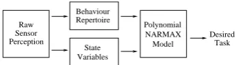
Phase 2: The controllers obtained at phase 1 are loaded to the robot in order to form a behaviour repertoire in the robot’s memory. For more complex tasks, we obtain a model using the NARMAX system identification methodology, which models the new task as a function of these previously acquired behaviours. Here, the composition of behaviours is done using state variables which contain information about the state of the environment and the robot (see figure 2).

Behaviour Repertoire

Desired Task Variables

State Perception

Sensor

Raw Polynomial

NARMAX Model

Fig. 2. The bootstrapping method of generating complex robot training

tasks.

Phase 3: Once we obtain the model, we test it on the robot in order to validate performance. If the new controller is successfull it is added to the repertoire so that it can be used to generate even higher level controllers in the future.

II. ARMAX/NARMAX MODELLING AND

EXPERIMENTALSETUP

a) Modelling Procedure: ARMAX (Auto-Regressive

Moving Average models with eXogenous inputs)

[Eykhoff, 1974], [Eykhoff, 1981] and NARMAX

(Nonlinear ARMAX) [Chen and Billings, 1989],

supervised parameter estimation methodologies for identifying both the important model terms and the parameters of unknown non-linear dynamic systems. These produce linear or nonlinear polynomial functions that model the relationship between some input and some output, both pertaining to the robot’s behaviour. A more detailed discussion of about the modelling technique is presented in [Korenberg et al., 1988], [Billings and Voon, 1986].

b) Experimental Setup: The experiments described in this paper were conducted in the 100 square meter circular

robotics arena of the University of Essex, using a Scitos

G5 mobile robot calledFOX. The robot is equipped with a

HOKUYO laser range finder. This sensor has a 4 m distance range, 240◦_{angular range and approximately 0.36}◦_angular

resolution. The robot also incorporates a colour video camera

with 640×480 pixels resolution which can deliver colour

images up to 60Hz.

III. SIMPLEBEHAVIOUR1: OBSTACLEAVOIDANCE

In the first experiment, we trainedFOX, to avoid obstacles towards the “obvious” side as shown in figure 3; if robot has more space on the right side, it turns to right, and if there is more space on the left, it turns to left.

OBSTACLE

ROBOT

OBSTACLE

ROBOT

(a) (b)

Fig. 3. Experiment 1. The desired obstacle avoidance behaviour. The

robot must choose the “obvious” side to avoid the obstacle in front. While approaching to the boxes if robot has more space on the right side, it turns right (b) and if there is more space on the left, it turns to the left (b).

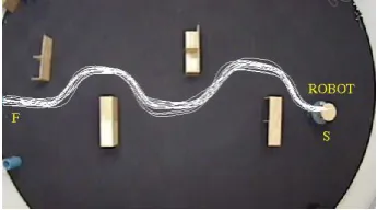
In order to teach the desired behaviour to FOX, the

programmer drove the robot in the training environment (figure 4) avoiding obstacles by turning the robot to the side having more space. During the experiments, the robot was started from the initial position S and stopped at the destination point F for 16 times. During each run, laser readings and the motor commands of the robot were logged in every 250 ms.

Having obtained the training data, we coarse coded laser readings into 11 sectors by averaging 62 readings for each

22◦ _{intervals. Coarse coded laser readings were clipped at}

1._{5m to avoid models taking far-away obstacles into account} that are irrelevant to obstacle avoidance.

We then modelled the angular velocity ω_o of the robot

as a function of coarse coded laser readings (u1−u11)

using ARMAX system identification methodology where the initial training parameters were Nu=0, Ny=0 and l=1.

The obtained model was a linear polynomial with 6 terms (table I).

Fig. 4. Experiment 1. The trajectory of the robot guided by the programmer. The robot was started from point S and avoided boxes along the route until it reaches the destination point F. The experiment was repeated 16 times and for each run the laser readings and the motor commands of the robot were logged in every 250ms. Note that trajectories of the robot was obtained using aViconmotion tracking system mounted in the arena which can deliver 3D data upto 100Hz with an accuracy better than 1mm.

ω_{o(n) = +0}.183−0.187·u4(n)−0.137·u5(n)

−0.021·u6(n)−0.045·u7(n) +0.265·u8(n)

TABLE I

EXPERIMENT1. THEARMAXMODEL LINKING THE LASER

PERCEPTION TO THE ANGULAR VELOCITY OF THE ROBOT FOR

AVOIDANCE BEHAVIOUR.

c) Model validation: We tested the steering speed model on the robot in three different test environments. During the experiments the linear speed of the robot was clamped to 0.1m/s.

In the first test environment, the robot was started from 20 different initial positions in front of two boxes put next to each other and was expected to avoid them from the “obvious” side where the robot had more space. The results (figure 5(a)) confirmed the expectation where the robot was able to avoid obstacles as desired.

1

(a) (b) (c)

Fig. 5. Experiment 1. The three environments where the obtained angular

speed modelω_{ogiven in table I was tested for obstacle avoidance behaviour.}

The results show thatω_{owas captured the general relationship between the}

laser perception and the motor commands of the robot to achieve the obstacle avoidance behaviour.

In the second (figure 5(b)) and third (figure 5(b)) test

1_{In three runs out of 20, when the robot was started from the mid-point}

environments, we tested if the obtained angular speed model captured the real essence of obstacle avoidance behaviour. The robot was started in front of the boxes arranged to simulate a right and a left corner and in both cases the robot was successfull to avoid the corners by turning the “obvious” side. Note that for both environment the robot was started from 16 different initial positions.

IV. SIMPLEBEHAVIOUR2: LEFT/RIGHTTURNING

ACCORDING TO THECOLOUR OF THEOBSTACLE

In the second experiment, we trained FOX in such a

way that it determined the turning direction according to the colour of the obstacle rather than choosing the

“obvi-ous” side. The experimental scenario here is: while FOX

approaches to an obstacle, it identifies the colour of the obstacle by a simple colour filtering algorithm, then i) if the colour of the obstacle is red, the robot avoids the obstacle by turning to right, and ii) if the colour of the obstacle is green, the robot escapes the obstacle by turning to left.

In order to obtain the training data set, we drove the robot in two environments: i) the first one contained boxes of red colour, where the robot was avoiding them by turning to right (figure 6(a)) and ii) the second environment contained green boxes where the robot was avoiding them by turning to left (figure 6(b)). In each environment, we conducted the experiments 10 times starting the robot from initial point S, stopping at the final point F.

(a) (b)

Fig. 6. Experiment 2. The trajectories of the robot in two training

environments; i) the first one contained boxes with red colour where the robot was avoiding them by turning to right (a) and ii) the second environment contained green boxes where the robot was avoiding them by turning to left (b))

During the experiments, we logged the coarse coded laser readings and the motor responses of the robot as well as the colour indexci(ci=1 for green,ci=2 for red boxes) of the

closest obstacle to the robot every 250 ms.

After logging this perception-action data, we modelled

the angular speed ω_{t of the robot using NARMAX system}

identification methodology as a function of the coarse coded laser readings (u1−u11) and the colour index of the detected

obstacle (ci). The initial training parameters were Nu =

0, Ny=0 and l =2 and the resultant NARMAX model

contained 21 terms (table II).

The resultant polynomial model ω_t is essentially the

combination of two polynomials, where each polynomial turns the robot to a different direction, and the transition between the two is performed using the terms including state variableci (the last two rows in table II).

ω_{t(n) = +3}.839−0.661·u4(n)−0.212·u5(n)

+0.650·u7(n)−2.413·u8(n)−0.093·u4(n)2

+0.150·u5(n)2−0.002·u7(n)2+0.050·u8(n)2

−0.202·u4(n)·u5(n)−0.098·u4(n)·u6(n)

−0.546·u4(n)·u7(n) +1.121·u4(n)·u8(n)

−0.249·u5(n)·u6(n) +0.076·u5(n)·u7(n)

−0.129·u6(n)·u7(n) +0.130·u6(n)·u8(n)

−1.469·ci(n) +0.263·ci(n)·u5(n)

+0.369·ci(n)·u6(n) +0.280·ci(n)∗u7(n)

TABLE II

EXPERIMENT2. THENARMAXMODEL FOR THE ANGULAR SPEED OF

THE ROBOT. THE MODEL IS A SECOND ORDER POLYNOMIAL INCLUDING

18TERMS. THE LAST TWO ROWS SHOW THE TERMS INCLUDING STATE

VARIABLEci.

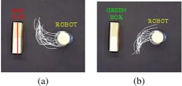
d) Model validation: As before we validated the per-formance of the obtained angular speed model by testing it on the robot. We put the robot in front of red and green boxes and let the model drive the robot. For each coloured box, the model was tested 16 times and the resultant trajectories of the robot are given in figure 7. They confirm that the model given in table II achieves the desired behaviour.

(a) (b)

Fig. 7. Experiment 2. The resultant trajectories of the robot guided by the

angular speed modelω_{t when it is confronting the: (a) red coloured boxes}

and (b) green coloured boxes. The results show that the obtained angular speed model was successful making the robot to turn the right direction according to the colour of the detected obstacle.

In order to quantify the performance of the angular speed

model ω_{t, we computed the strength of the association}

be-tween the colour of the detected obstacle and the direction of

the corresponding turning speed of the robot usingCramer’s

Vtest. To do so, we checked the sign of the resultant turning speed according to the colour of the detected obstacle during the test runs. When the robot detected a green obstacle, the resultantω_t>0 (indicating to turn left) 97.651% of the time, and when the detected obstacle is red,ω_t<0 (indicating to

turn right) 98._{837% of the time. The results showed that}

there is a significant correlation whereV=0._{96. Note that}

V varies between 0 and 1 corresponding to no association

and perfect association respectively.

V. COMPLEXBEHAVIOUR1: ROUTELEARNING

transition between behaviours is done using state variables containing information about the current state of the envi-ronment. We will now show that this can be used to achieve more complex tasks.

Scaling up from the first two experiments, the third task

was to generate a polynomial which can guideFOXto follow

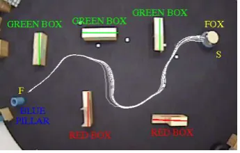
a particular route in order to reach a desired object. The experimental scenario is given in figure 8, the environment is populated with red and green boxes in order to guide the robot to the destination pointF, where the target object, blue pillar, is present.

60 cm 100 cm

ROBOT

PILLAR

RED BOX

GREEN BOX GREEN BOX

RED BOX

GREEN BOX

F

S

Fig. 8. Experiment 3. The experimental scenario where the desired task

is to teach the robot to follow a particular route in order to reach the blue pillar. Note that the environment is populated with red and green boxes to indicate the right direction to the robot to follow.

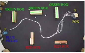
To collect the training data, the programmer drove the robot manually in the target environment (figure 9) 10 times starting the robot from the initial positionSand stopping the robot in front of the blue pillar (destination pointF). During the training, laser readings, camera images and the motor commands of the robot were logged in every 250 ms.

Fig. 9. Experiment 3. The trajectories of the robot guided manually by

the human operator in order to obtain the training data.

A. Bootstrapping from Low-Level Controllers

After logging the training data, as discussed in section I-A, we processed the laser readings and the raw images to extract three low level controllers which will then be fed to polynomial NARMAX models as inputs. These controllers are:

• Obstacle avoidance controller The first controller in

the behaviour repertoire guides the robot to avoid

ob-stacles. Here we used the polynomial model ω_o given

in table I obtained in experiment 1 (section III).

• Colour encoded turning controller The second one

turns the robot to right if the colour of the detected object is red and it turns the robot to left if the colour

is green. Here we used the polynomial model ω_{t given}

in table II, obtained during experiment 2 (section IV).

• Object seeking controller: We also implemented a

simple object seeking controller which looks for the nearest object in front of the robot and guides the robot towards it.

Having identified the controllers, we also obtained three state variables which will help the system identification process to link the low level controllers in order to achieve the desired task:

• di defines if the target object is detected or not; d=

0 represents target object is not detected, and di =1

represents target object is detected.

• oidefines if there is an obstacle close to the robot;oi=

0 represents there is no obstacle detected, and oi=1

represents the presence of an obstacle.

• ci states the colour of the detected obstacle; ci =1

represents green, ci =2 represents red, and ci = 0

represents all other colours.

e) Obtaining Polynomial Models: We then obtained

two polynomial models; one for the linear speedvr and one

for the angular speedω_r of the robot — as a function of the predefined behaviours (ω_o,ω_t andω_w) and the state variables (di,oi andci). The obtained models are given in table III.

vr(n) = +0.100−0._100·di(n) ω_r(_n) = +₀._{100·d(n) +1}._000·ω_w(_n)

−1._000·oi(n)·ω_w(_n) +₁._000·oi(n)·ω_o(_n)

−1.000·oi(n)·ci(n)·ω_o(n) +1.000·oi(n)·ci(n)·ω_t(n) +1.000·di(n)·oi(n)·ω_w(n)−1.000·di(n)·oi(n)·ω_o(n) +1.000·di(n)·oi(n)·ci(n)·ω_o(n)

−1.000·di(n)·oi(n)·ci(n)·ω_t(_n)

TABLE III

EXPERIMENT3. THE POLYNOMIAL MODELS FOR THE LINEARvrAND

ANGULAR SPEEDω_{rOF THE ROBOT.}

f) Models Validation: Having obtained the perception models vr andω_r, we tested them on the robot. We let the models drive the robot in the target environment 10 times. Figure 10 shows the resultant trajectories, where in each run the robot was successful to reach the target object.

VI. EXTENDEDBOOTSRAPPINGMETHOD

In experiment 3 we have demonstrated how simple NAR-MAX models can be used to achieve more complex tasks. One interesting question here is “what happens if the low level controllers found in the behaviour repertoire are not adequate to generate the desired task?”

Fig. 10. Experiment 3. The trajectories of the robot under the control of the perception models given in table III. The results show that the robot successfully reached the target object in each run.

data is controlled according to the state of the environment and the robot (figure 11).

Behaviour Repertoire

Perception Sensor

Raw

Model NARMAX Polynomial

Variables State

Desired Output

Fig. 11. The extended bootstrapping method of generating complex robot

training tasks. In the extended version we also give raw sensory data as inputs to the system.

A. Complex Behaviour 2: Modelling Complex Route Learn-ing Task

To demonstrate the extended method, we taught FOX to

follow a complex route of different stages (figure 12). First, the robot has to reach a blue pillar by correctly following the coloured objects. Once it reaches the pillar, it has to wait with zero linear and angular speeds until the pillar is removed from the environment (stage 2). Once the pillar is removed, the robot must complete the route by traversing the two consecutive door-like openings with 1 m wide each to reach the destination point F.

GREEN BOX

RED BOX PILLAR

1m

1m

2m 2m

ROBOT

S

F

W BOX

BOX

BOX BOX

Fig. 12. Experiment 4. The experimental scenario for the desired complex

route learning task.

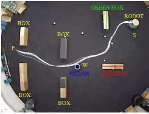
As before we obtained the training data by driving the robot manually in the target environment shown in figure 13. Starting the robot at initial position S, first we drove the robot to point W. Then the robot was stopped in front of the pillar until the pillar was removed by the human operator. We then

continued driving the robot to pass through two consecutive door-like openings. The experiments were repeated 10 times and for each run we logged the laser perception, camera images and the motor commands of the robot in every 250 ms.

Fig. 13. Experiment 4. The trajectories of the robot under the manual

control of the human operator training data collection.

g) Obtaining Sensor Based Models: After logging the training data, we fed the raw perception data to low-level controllers present in the behaviour repertoire of the robot to generate higher level inputs for the desired task. But this time we also coarse coded the laser readings into 11 sectors (u1 to u11) by averaging 62 readings for each 22◦ in order

to enrich the system inputs, since there is no ready door traversing controller in the behaviour repertoire of the robot. Also for the transition between the behaviours, we computed a state flag si which indicates if the blue pillar is removed

from the front of the robot (si=1) or not (si=0 ).

We then obtained two polynomial modelsvcandω_cusing

NARMAX system identification methodology as a function coarse coded laser readings (u1−u11), route following

con-trollers vr andωr obtained in section V, and state variable si. The obtained models are given in table IV.

vc(n) = vr+0.1·si(n)

ω_{c(n) = −0}.033+1.016·ω_{r(n) +0}.144·u4(n)

−0.088·u5(n) +0.004·u6(n)−0.131·u7(n)

+0._{014·u8(n) +0}._208·ω2

r(n)−0.026·u24(n)

+0.029·u25(n) +0.062·u27(n)2−0.025·u4(n)·u8(n)

+0.394·si(n)−1.051·si(n)·ω_r(_n)

−0.145·si(n)·u4(n)−0.060·si(n)·u5(n)

−0.040·si(n)·u6(n) +0.026·si(n)·u7(n)

TABLE IV

EXPERIMENT4. THE POLYNOMIAL MODELS FOR THE LINEAR AND

ANGULAR SPEED OF THE ROBOT FOR COMPLEX ROUTE LEARNING

BEHAVIOUR. THE LAST THREE ROWS SHOW THE TERMS INCLUDING

STATE VARIABLEsi.

where the robot completed the track successfully in each attempt.

Fig. 14. Experiment 4. The trajectory of the robot under the control of

the perception models given in table IV. The experiments were repeated 10 times and for each run the robot completed the track successfully to reach the destination point F without bumping into the boxes in each attempt.

Transparent Models: Having transparent models like the ones given in table IV has a number of advantages, for example the possibility to analyse the robot behaviour formally. Here, for instance, one can see that the model

of table IV ω_c has two components. The first one is the

colour based route following behaviour which was previously obtained in section V, taking the control of the robot when state flagsiequals 0. The second behaviour is a door traversal

controller activated whensi=1.

The separability of the behaviours enabled us to add door traversal controller to the behaviour repertoire of the robot. In this way we do not only obtain models to achieve the desired task, but we also extract new low level controllers from the polynomial model in order to enrich the behaviour repertoire of the robot.

VII. CONCLUSION ANDFUTUREWORK

This paper introduces a bootstrapping method of gener-ating complex robot training tasks using polynomial NAR-MAX structures. The method is based on obtaining hierar-chical polynomial models which model the desired task by combining predefined low level sensor motor controllers and raw sensory data in a judicious way.

The method uses the advantage of polynomial models being truly linear in the parameters [Chen et al., 1990]. This allows us to combine different low level controllers in a single polynomial in order to achieve more complex tasks. The transition between these controllers is done using state variables which contain information about the state of the environment.

ACKNOWLEDGMENTS

We express our thanks to Emre ¨Ozbilge for his

contri-bution to this paper. We also gratefully acknowledge that the RobotMODIC project is supported by the Engineer-ing and Physical Sciences Research Council under grant GR/S30955/01.

REFERENCES

[Akanyeti et al., 2007a] Akanyeti, O., Kyriacou, T., Nehmzow, U., Iglesias, R., and Billings, S. (2007a). Visual task identification and

characterisa-tion using polynomial models. Robotics and Autonomous Systems.

[Akanyeti et al., 2007b] Akanyeti, O., Nehmzow, U., Weinrich, C., Kyria-cou, T., and Billings, S. (2007b). Programming mobile robots by

demon-stration through system identification. InECMR, Freiburg, Germany.

[Billings and Chen, 1998] Billings, S. and Chen, S. (1998). The deter-mination of multivariable nonlinear models for dynamical systems. In

Leonides, C., (Ed.),Neural Network Systems, Techniques and

Applica-tions, pages 231–278. Academic press.

[Billings and Voon, 1986] Billings, S. and Voon, W. S. F. (1986).

Corre-lation based model validity tests for non-linear models. International

Journal of Control, 44:235–244.

[Chen and Billings, 1989] Chen, S. and Billings, S. (1989).

Representa-tions of non-linear systems: The narmax model. International Journal

of Control, 49:1013–1032.

[Chen et al., 1990] Chen, S., Billings, S. A., Cowan, C. F. N., and Grant, P. M. (1990). Practical identification of narmax models using radial basis

functions. International Journal of Control, 56:6:1327–1350.

[Demiris and Hayes, 1996] Demiris, J. and Hayes, G. (1996). Imitative

learning mechanisms in robots and humans. In Proc. 5th European

Workshop on Learning Robots, pages 9–16, Bari, Italy.

[Eykhoff, 1974] Eykhoff, P. (1974). System Identification: parameter and

state estimation. Wiley-Interscience, London.

[Eykhoff, 1981] Eykhoff, P. (1981). Trends and Progress in System

Identification. Pergamon Press.

[Korenberg et al., 1988] Korenberg, M., Billings, S., Liu, Y. P., and McIl-roy, P. J. (1988). Orthogonal parameter estimation algorithm for

non-linear stochastic systems.International Journal of Control, 48:193–210.

[Nehmzow et al., 2005] Nehmzow, U., Kyriacou, T., Iglesias, R., and Billings, S. (2005). Self-localisation through system identification. In Proc. of ECMR 05 - European Conference on Mobile Robots 2005. Springer Verlag.

[Nguyen and Widrow, 1990] Nguyen, D. and Widrow, B. (1990). The

truck-backer upper: An example of self-learning in neural networks. IEEE Control Systems Magazine, 10:2:18–23.

[Pomerleau, 1993] Pomerleau, D. (1993).Neural Network Vision for Robot