Theoretical and numerical estimation of ship-to-ship hydrodynamic interaction effects

Theoretical and numerical estimation of ship-to-ship hydrodynamic

interaction effects

Zhi-Ming Yuan

a

, Chun-Yan Ji

b,n

, Atilla Incecik

a

, Wenhua Zhao

c

, Alexander Day

a a

Department of Naval Architecture, Ocean and Marine Engineering, University of Strathclyde, Glasgow, UK

b_{School of Naval Architecture and Ocean Engineering, Jiangsu University of Science and Technology, Zhenjiang, China} c

Centre for Offshore Foundation Systems (M053), The University of Western Australia, 35 Stirling Highway, Crawley, WA 6009, Australia

a r t i c l e i n f o

Article history:

Received 8 May 2015 Received in revised form 9 May 2016

Accepted 17 May 2016

Keywords:

Hydrodynamic interaction Rankine source method Far-field wave pattern Boundary element method Ship-to-ship problem Forward speed effects

a b s t r a c t

The main objective of this paper is to investigate theoretically and numerically how much interactions are expected between two ships travelling in waves. The theoretical estimation is based on asymptotic far-field wave patterns produced by a translating and oscillating source. The far-field wave pattern is governed by the parameter

τ

¼

ω

eu0/g;For values of the parameter

τ

40.25 there exist a fan-shaped quiescent region in front of the vessel. As

τ

increases,the range of the fan-shaped quiescent region will be expanded. The critical line between the quiescent and wake region can be estimated by the asymptotic expressions theoretically. It is expected that there is no hydrodynamic interaction if the two ships are located in each other's fan-shaped quiescent region. But due to the near-field local waves produced by the 3-D ships, the critical line could be different from that estimated from asymptotic wave pattern. Therefore, we developed a 3-D panel method based on Rankine-type Green function to in-vestigate the hydrodynamic interaction effects for several combinations of parameters, including oscil-lation frequency, forward speed and transverse distance between two ships. Finally, the critical line calculated numerically was presented and compared to the theoretical estimation.

&2016 The Authors. Published by Elsevier Ltd. This is an open access article under the CC BY license (http://creativecommons.org/licenses/by/4.0/).

1. Introduction

Interest in the prediction of the hydrodynamic interactions between two advancing ships has grown in recent years as the ships have to pass each other in close proximity in harbour areas and waterways with dense shipping traffic. The behaviour of two ships in waves with speed effect is of special concern to the Navy, that is, for underway replenishment, and for other commercial purposes.

Fang and Kim (1986) firstly took forward speed into con-sideration in ship-to-ship problem. They utilized a 2-D procedure, including the hydrodynamic interaction and an integral equation method, to predict the coupled motions between two ships ad-vancing in oblique seas. They found that the roll motion was re-duced while the ships were advancing. However, due to the 2-D assumptions, some deficiencies including the special treatment of the convective term still exist. Chen and Fang (2001) extended Fang's method (Fang and Kim, 1986) to 3-D. They used a 3-D Green function method to investigate the hydrodynamic problems be-tween two moving ships in waves. It was found that the

hydrodynamic interactions calculated by 3-D method were more reasonable in the resonance region, where the responses were not as significant as predicted by 2-D method. However, their method was only validated by model tests with zero speed. More rigorous validation should be carried out by further experiments. McTag-gart et al. (2003)andLi (2007)used the model test data fromLi (2001)to verify their numerical programmes, which was based on 3-D Green function method. The numerical predictions and ex-periments showed that the presence of a larger ship could sig-nificantly influence the motions of a smaller ship in close proxi-mity. But the numerical prediction of roll motion was not accurate.

Xu and Faltinsen (2011) used the model test data from Ronæss (2002)to verify their numerical programme based on 3-D Rankine source method. They applied an artificial numerical beach to sa-tisfy the radiation condition. They found that the hydrodynamic peaks and spikes were related to the resonance modes in the gap between the hulls. However, they also failed to predict the roll motion precisely. Within the frame work of Green function,Xu and Dong (2013)developed a 3-D translating-pulsating (3DTP) source method to calculate wave loads and free motions of two ships advancing in waves. Model tests were carried out to measure the wave loads and the free motions for a pair of side-by-side arranged ship models advancing with an identical speed in head regular waves. Both the experimental and the numerical predictions Contents lists available atScienceDirect

journal homepage:www.elsevier.com/locate/oceaneng

Ocean Engineering

http://dx.doi.org/10.1016/j.oceaneng.2016.05.032

0029-8018/&2016 The Authors. Published by Elsevier Ltd. This is an open access article under the CC BY license (http://creativecommons.org/licenses/by/4.0/).

n_{Corresponding author.}

showed that hydrodynamic interaction effects on wave loads and free motions were significant. Most recently,Yuan et al. (2015a,

2014a,2015b)developed a 3-D Rankine source panel method to investigate the hydrodynamic interactions between two ships travelling in shallow water. They used a new modified Sommerfeld radiation condition which was applicable to a wide range of for-ward speeds, including very low forfor-ward speed problem where the parameter

τ

(

τ

¼

ω

eu0/g,

ω

e is the encounter frequency,u0 is the forward speed, and g is the gravity acceleration) is smaller than 0.25. Their method was validated through model experi-ments and a very large sway force was predicted when the transverse distance between two ships equalled to the wave-length. They also found that the hydrodynamic interactions be-tween two ships were caused by the scattered waves.

The hydrodynamic interaction between two advancing ships is very important. Because of the hydrodynamic interactions, even relatively small wave can induce large motions of the smaller ship due to the nearness of the larger ship. In order to minimize the hydrodynamic interactions, we attempt to establish a rapid ap-proach tofind the relationship between the minimum spacing and the parameter

τ

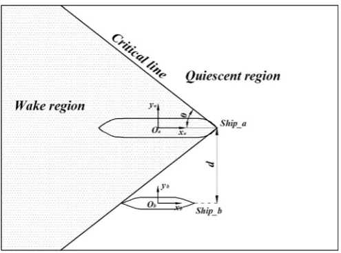
. The minimum spacing here is referred as the minimum transverse distance between two ships that the hydro-dynamic interaction is not expected. The optimum hull spacing of a family of multihulls was firstly investigated by Tuck and La-zauskas (1998). They used a thin-ship theory to optimize the multihull con_figurations for minimum wave-making. The opti-mum configurations were determined for two, three and four-hulled vessels, with and without longitudinal stagger. The gener-ated wave amplitude, wave resistance and total drag were calcu-lated and compared in their study.Battistin (2000)andYang et al. (2002)also carried out hydrodynamic optimization for a trimaran. However, these studies mainly considered the calm-water case, in order to minimise wave making.Day and Doctors (2001) devel-oped a rapid method to estimate the near- and far-field wave wake. They applied this method to the optimization of a monohull and a catamaran. But the multihulls were treated as a rigid body with 6 degrees of freedom (DoF). No attempt was made to opti-mise the hydrodynamic interactions between two ships (12 DoF) advancing in waves, since the motions of the ships could make the problem more complex. The main aim of the study presented in this paper is to establish a rapid method to evaluate the hydro-dynamic interaction between two ships advancing in waves, in order to provide an optimum configuration of two ships. No at-tempt is made here to optimise the shape of individual hulls.

2. Theoretical estimation of the critical line

2.1. Background

For a single marine vessel advancing in calm-water, the so-called Kelvin wake can be observed. It is set up by a ship in steady motion and to be confined within a wedge of semi-angle sin1_{(1/3) in deep water. Lighthill (1978) used the stationary} phase method to investigate this Kelvin angle. It can be observed from the Kelvin wake that the free surface can be divided into two regions by a critical line: wake region confined within the Kelvin angle and quiescent region outside the Kelvin angle. For the ships travelling in waves, except the Kelvin wave system, there exist two (

τ

40.25) or three (

τ

o0.25) unsteady wave systems due to the oscillation of the ship (Becker, 1958;Wehausen, 1960).

Similar to the steady wave problem, the free surface of an os-cillating and translating body can also be divided into two regions: wake region confined within a semi-wedge angle

θ

and quiescent region outside

θ

. However, for the unsteady ship motion, the range of the wedge is not a constant value. It varies with the parameter

τ

(Lighthill, 1967;Noblesse, 2001;Noblesse and Hendrix, 1992). For the parameter

τ

40.25, there exists a fan-shape quiescent region in front of the vessel. As

τ

increases, the range of the fan-shape quiescent region will be expanded.Kashiwagi and Ohkusu (1989,

1991)used the asymptotic wave contour to estimate the side-wall effect. They also extendedNewman (1978) uni_fied slender-ship theory and developed a new method to calculate the side-wall effect numerically. The critical line obtained numerically was presented and compared to the results estimated from asymptotic wave contour.Faltinsen (2006)derived a wave angle to investigate the wave interference between the waves generated by each hull of a multihull vessel. However, this wave angle was not validated from numerical calculation. In order to investigate how much the hydrodynamic interaction would be minimised if Ship_b is located in the quiescent region of Ship_a (as shown inFig. 1), a massive numerical calculations are required to analyse several combina-tions of parameters, including oscillation frequency, forward speed and transverse distance between two ships. This is the main ob-jective of the present study. Before the numerical calculation, a theoretical estimation should be established based on the asymptotic wave contour. In the present paper, we will use the Havelock form of Green function to investigate the far-field wave patterns generated by a translating and oscillating source in

in-finite water depth and then establish a rapid estimation of the critical line between the quiescent and wake region.

2.2. Far-field wave patterns

In order to obtain the critical line between the quiescent and wake region, the formulations of far-field asymptotic wave pat-terns should be established. The far-field unsteady wave pattern had been made more than half a century ago byHanaoka (1953)

[image:2.595.304.552.55.239.2]

and Eggers (1957). Becker (1958) also investigated the far-field wave pattern produced by a harmonic pulsating source. He pro-vided a curves of equal phase for the various systems of waves formed. The 3-D frequency-domain analysis of theflow about a ship advancing in waves was pioneered byChang (1977). Similar numerical work can be found byInglis and Price (1982),Wu and Eatock Taylor (1987,1989),Rahman (1990), Iwashita (1997). No-blesse and Hendrix (1992)derived the far-field wave patterns of a ship advancing in waves by using a stationary phase method. They derived the so-called cusp angle for different wave systems. The far-field behaviour of a 3-D pulsating source of Michell type with forward speed was also studied byMiao et al. (1995)by using the Fourier transformation and contour integration technique. More recent research on far-field wave patterns and their characteristics

were presented byXu et al. (2013)by using a Havelock form Green function method.

According toIwashita (1997)andXu et al. (2013), the Havelock form of Green function is given in the following form

⎛ ⎝ ⎜ ⎞ ⎠ ⎟ π π = − ′ + ( ) ( ) G

r r k T X Y Z

1 4

1 1 i

2 0 , , 1

where

}

′ = ( − ′) + ( − ′) + ( ∓ ′) ( )

r

r x x 2 y y 2 z z 2 2

⎡ ⎣⎢ ⎤⎦⎥ ⎡ ⎣⎢ ⎤ ⎦⎥

∫

∑

π ϖ

τ θ θ

∇ ( ) = − ( − ) ∇ ( ) − _{( )} π = −

T X Y Z k

I k d

1 _{, ,} i

2 1

1

1 4 cos ₃

i j i

ij i j

0 , 1 2 1 0 ⎡ ⎣ ⎢ ⎢ ⎢ ⎤ ⎦ ⎥ ⎥ ⎥ ⎡ ⎣ ⎢ ⎢ ⎤ ⎦ ⎥ ⎥ ⎡⎣ ⎤⎦ ⎡ ⎣ ⎤⎦ ⎫ ⎬ ⎪ ⎪ ⎪ ⎪⎪ ⎭ ⎪ ⎪ ⎪ ⎪ ⎪ _{( )} ϖ ϖ ϖ θ θ ϖ ϖ

ϖ ϖ π

θ τ θ τ θ

( ) = ( ) ∇ ( ) = ( − ) ( ) − ( ) ≡ ( ) + = − + ( − ) − ( = = ) ϖ − 4

I k k F k

I k k F k

k F k e E k iH k

i j

i cos 1 i sin

1

1

2 1

2 cos 1 2 cos 1 1 4 cos

1, 2; 1, 2 ,

ij i j i i j

ij i j j i i j

i j

i j ki j i j ij

i i

0

1 2 ₀

0 1

2

⎡⎣ ⎤⎦

ϖ = + θ+ ( − ) θ = ( ′ + )

= ( − ′) = ′ −

−

Z X Y Z k z z

X k x x Y k y y

i cos 1 sin , ,

,

j j 1 0

0 0

∫

ϖ ( ) = = ϖ ∞ −

E k e

t dt k

g u , i j k t 1 0 02 i j

The control factors are defined as

⎪ ⎪ ⎪ ⎪ ⎧ ⎨ ⎩ ⎧ ⎨ ⎩ ⎡⎣ ⎤⎦ ϖ ϖ ϖ ϖ ϖ

ϖ θ ν

= − ( ) ≤ ( ) <

( ) <

= ( ) ≤ ( ) >

( ) ≤ ∈

H k k

k

H k k

k

1 Re 0, Im 0

0 Im 0 ,

1 Re 0, Im 0

0 Im 0 , 0, ;

j j j j j j j j 1 1 1 1 1 2 2 2 ⎪ ⎪ ⎪ ⎪ ⎧ ⎨ ⎩ ⎧ ⎨ ⎩ ⎡ ⎣⎢ ⎤⎦⎥ ϖ ϖ ϖ

ϖ θ ν

π = ( ) <

( ) < =

− ( ) ≤

( ) > ∈

H k

k H

k k

1 Im 0

0 Im 0,

1 Im 0

0 Im 0 , 2 ;

j j j j j j 1 1 1 2 2 2 ⎪ ⎪ ⎪ ⎪ ⎧ ⎨ ⎩ ⎧ ⎨ ⎩ ⎡ ⎣⎢ ⎤⎦⎥ ϖ ϖ ϖ ϖ θ π π = ( ) ≥

( ) < =

( ) ≥ ( ) < ∈

H k

k H

k k

1 Im 0

0 Im 0,

1 Im 0

0 Im 0 2,

j j j j j j 1 1 1 2 2 2

(x, y, z) and (x′, y', z′) denotes the position vector of thefield point and source point respectively. Then the free-surface eleva-tion can be expressed as

⎡⎣ ⎤⎦ ⎡ ⎣ ⎢ ⎛_⎝⎜ ⎞_⎠⎟ ⎤ ⎦ ⎥ ζ Ξ ω ( ′ ′ ′ ) = ( ′ ′ ′) = + ∂ ∂ ( ) ω ω − = − =

x y x y z t x y x y z e

g i G u

G x e

, , , , , Re , , , ,

Re 1

5

i t z

e i t

z 0 0 0 e e

where

Ξ

is the spatial expression of the free-surface elevation. By substituting Eqs.(1)–(4)into Eq.(5), the time independent wave shape function can be written as

∫

∫

∫

∫

∫

∑

∑

∑

∑

∑

( )

ζ θ θ θ θ θ θ

θ θ θ θ

( ′ ′ ′) = ( ) + ( ) + ( ) + ( ) + ( ) ν ν ν π ν π π π = = =

= = 6

x y x y z F d F d F d F d F d

, , , , j j j j j j j j j j 1 2

0 1 ₁ 2

0 2 ₁ 2 1 1 2 _/2 2 1 2 /2 2 where ⎡⎣ ⎤⎦ ( ) θ

ω ϖ θ ϖ ϖ

π τ θ

( ) = ( − ) ( ) + ( ( ) − ) − − − 7

F k k F k u k F k k

g

1 i cos

4 1 4 cos

ij i

i e j j i j

1 0 0 0 0 0

1 2 ⎧ ⎨ ⎪ ⎩ ⎪ ⎛_⎝⎜ ⎞_⎠⎟ ν τ τ τ =

( < )

( > )

( ) −

0, 0.25

cos 1

4 , 0.25 8

1

In the far-field, asX2_þY2_-1,ekϖ_{E k( ϖ)}

j

1

j _and

ϖ

1

in Eq.(4)tend to be zero (Takagi, 1992), and Eq.(7)can be reduced to

θ ω θ

π τ θ

( ) = ( − ) ( + )

− ( )

ψ

+

F k k H u k k

g e

1 cos

2 1 4 cos 9

ij i

i ij e i _{k Z i}

0 0 0

i ij

The phase function ψ can be defined as

⎡⎣ ⎤⎦

ψ =_{k X cos} θ+ ( − )₁ −_{Y sin} θ _{( )}

10

ij i j 1

By denoting κi= −ki cos θ when ωe≠0and u≠0(the

dis-cussion on the case of ωe=0and u=0can be found inXu et al.

(2013)), Eq.(9)can be written as

κ κ τ ω κ

π κ τ

( ) = ( − ) ( − )

( + ) ( )

κ τ ψ

( − ) +

F k H uk

g e

2 11

ij i i ij e i

i

Z i

0 3 0

i 2 ij

where

ψ = −_Xκ + ( − )₁ −_Y (κ − ) −τ κ _{( )}

12

ij i j 1 i 4 i2

It is well known within the frame work of stationary phase method that the main contribution to the wave term comes from the points where dψij/dκi=0in the far-field asX2þY2-1. Thus, we can obtain the following expression:

⎡⎣ κ τ κ⎤⎦

κ τ κ

= ( − ) ( − ) −

( − ) − ( )

−

X 1 Y 2

13

j i i

i i

1

3

4 2

Let the source point locate at (x′, y′, z′)¼(0, 0, z′), zo0. By substituting Eq.(13)into Eq.(12), the parametric equations can be expressed as ⎫ ⎬ ⎪ ⎪ ⎭ ⎪ ⎪

ψ κ τ κ

κ τ κ τ

ψ κ τ κ

κ τ κ τ

= ( − ) − ( − ) ( + ) = ( − ) ( − ) − ( − ) ( + ) ( ) k x k y 2 1 14 ij i i i i j ij i i i i 0 3 3 0 4 2 3

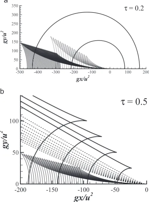
The constant-phase curves defined by Eq.(14)are depicted in

Fig. 2for a set of values ofψijwith increment equal to 2

π

. It can be

found inFig. 2(a) that at

τ

o0.25, there are three distinct wave systems: one ring wave system, which are approximately elliptical in shape, and two Kelvin fan wave systems confined within two distinct wedges, which can be referred as “outer and inner V waves”. The ring waves are dense in the positivex-axis and sparse in the negativex-axis. At

τ

40.25, as shown inFig. 2(b), the up-stream portion of the ring waves do not exist. The wave-pattern plots for values of

τ

_-0.25+_and

τ

_-0.25−_{can be found inNoblesse}

and Hendrix (1992). It should also be noted from Eq.(14)that only concentric circle ring waves will exist whenu0¼0, which presents the feature as a 3-D pulsating source without forward speed. An-other interestingfinding at the case ofu0≠0 and

ω

e¼0 is that the ring waves vanish and the inner and outer V waves merge together as Kelvin waves. Furthermore, as

κ

i-

τ

,x2þy2-1, and the in-tervals _1o

κ

io

τ

and

τ

o

κ

io

ν

5 (the value of

ν

5 will be discussed further on) corresponds to two branches of the fan waves, which can be called inner and outer fan waves respectively, as shown inFig. 3.

2.3. Semi-wedge angle and the minimum spacing

not exist, since the ring waves could cover the entire computa-tional domain. Therefore, in ship-to-ship problem, the minimum spacing cannot be identified and we are only concerned with the case of

τ

40.25 in the present study.

Fig. 3 shows the typical wave patterns at

τ

40.25. It can be observed that both of the ring waves and inner V waves have a cusp, which corresponds to the semi-wedge angle. Let's denote the coordinates of these cusps as (xr,yr) and (xi,yi) respectively, the corresponding semi-wedge angles can be written as

⎡

⎣ ⎢ ⎢

⎤

⎦ ⎥ ⎥ ⎡

⎣ ⎢ ⎢

⎤

⎦ ⎥ ⎥ ⎫

⎬ ⎪ ⎪ ⎪

⎭ ⎪ ⎪ ⎪

θ ν τ ν

ν τ ν

θ ν τ ν

ν τ ν

= ( − | | ) = − ( − ) − ( − ) −

= ( − | | ) = − ( − ) − ( − ) −

( )

− −

− −

y x

y x

tan / tan

2

tan / tan

2

15

r r r

i i i

1 1 5

4 52

5 3 5

1 1 6

4 62

6 3 6

The values of ν5andν6can be found inNoblesse and Hendrix

(1992)as

(

)

ν = − − + ( − ) + τ ± τ+ +

( )

c c

c

2 1 2 48

2 1 /2 16

5,6

2 2

where

⎡

⎣

(

)

(

)

⎤⎦

τ τ τ

= ( − ) + + − _{( )}

c 16 2 11/3 1 4 1/3 1 4 1/3 /2 ₁₇

It should also be noted that asκi-

τ

, the corresponding

semi-wedge angle for the inner fan wave could be expressed as ⎡

⎣

⎢ ⎤

⎦ ⎥ θ

τ

= ( − )

− ( )

− −

tan 1 1

16 1 18

f 1 j 1

2

The semi-wedge angles defined by Eqs.(15)and(18)are de-picted inFig. 4. The semi-wedge angle of the outer V waves is also presented. The expression of

θ

ois the same as that of

θ

r, as defined in Eq.(15). It should be noted that

θ

oonly exists at

τ

o0.25, while

θ

rand

θ

fexists at

τ

40.25. The semi-wedge angle of the inner V waves exists at the entire range of

τ

. It can also be observed from

Fig. 4that at

τ

_¼0, the semi-wedge angles of the outer and inner V waves merge together as Kelvin wedge 19.47°. When it refers to ship-to-ship problem, as shown inFig. 1, two values of

τ

are of particular interest:

τ

¼0.272 (the analytical expression is 2/27, which can be found inChen and Noblesse (1998)) and

τ

¼1.62. At

τ

o0.272, the semi-wedge angle

θ

r490°. In this case, the hydro-dynamic interactions between two ships are inevitable and the minimum spacing could not exist. Another critical case is

τ

¼1.62. As

τ

41.62, the semi-wedge angle

θ

ro19.47°. In this case, the hydrodynamic interactions and the minimum spacing are domi-nated by the steady waves. The quiescent region could exist out-side the Kelvin wedge. In the range of 0.272_o

τ

_o1.62, the quiescent region is deterred by

θ

r, since

θ

iand

θ

fare confined within the semi-wedge angle of the ring waves.

[image:4.595.37.281.61.392.2]

FromFig. 1, the minimum spacing between two ships with the same forward speed can easily be obtained. Let's denote the length of the larger and smaller ships as La and Lb respectively, the minimum spacing between two ships can be written as

[image:4.595.33.283.437.601.2] [image:4.595.306.551.552.723.2]

Fig. 2.Far-field wave patterns for a translating and pulsating source point located at (0, 0,z′),z′o0.(a)τ¼0.2; and (b)τ¼0.5.

Fig. 3.Typical wave patterns for the case ofτ40.25.

θ = ( + ) ( )

( )

d 1 L L

2 a b tan 19

Considering

θ

iand

θ

fare confined within the semi-wedge an-gle

θ

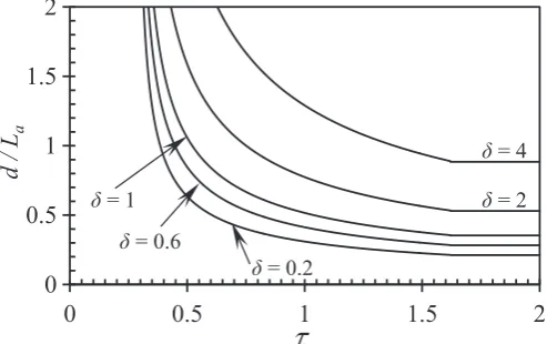
r, by substituting Eq. (15) into Eq. (19), the dimensionless minimum spacing can be written as

⎧

⎨ ⎪ ⎪⎪

⎩ ⎪ ⎪ ⎪

τ

δ ν τ ν

τ ν ν τ

δ τ

=

∞ ( ≤ )

( + ) ( − ) −

( − ) + ( < < )

( + ) ( ) ( ≥ )

( ) ∘

d L/

, 0.272

1

2 1 2 , 0.272 1.62

1

2 1 tan 19.47 , 1.62 20

a

5 4 52

53 5

whereδ=L Lb/ ais the ratio of the length of Ship_b to Ship_a, andν5 is defined in Eq.(16). From Eq.(20), it can be seen that the di-mensionless minimum spacing is only determined by

δ

and

τ

.

Fig. 5shows the dimensionless minimum spacing with different

δ

values. It can be observed that as the ratio of the length of Ship_b to Ship_a increases, the distance between the two ships must be increased to minimize the hydrodynamic interactions.

3. Numerical validations

In order to validate the present assumption, we used MHydro, which is based on 3-D Rankine source panel method, to in-vestigate the hydrodynamic properties of thefloating bodies.Yuan et al. (2015a,2014a)gave the details about using MHydro to solve the ship-to-ship with forward speed problem. The method de-veloped and the results obtained have been validated by experi-mental measurements. The same method and numerical pro-gramme will be used in the present study, and only some general descriptions about the numerical methodology will be summar-ized here.

3.1. Numerical methodology

The corresponding right-handed coordinate systems are shown inFig. 6. The body coordinate systemsoa-xayazaandob-xbybzbare

fixed on Ship_a and Ship_b respectively with their origins on the mean free surface, coinciding with the corresponding centre of gravity (CoG) in respect toxandycoordinates when both of the ships are at their static equilibrium positions.oa-zaandob-zbare both positive upward. The inertia coordinate system o-xyz with origin located on the calm free surface coincides with oa-xayaza when the ship has no unsteady motions.O-XYZis the earth-fixed coordinate system with its origin located on the calm free surface

and OZaxis positive upward. The incident wave direction is

de-fined as the angle between the wave propagation direction andX -axis.

β

¼180° corresponds to head sea;

β

¼90° corresponds to beam sea.ddenotes the transverse distance between two ships whileu0is the forward speed. In the computation, the motions and forces of Ship_a and Ship_b are concerted to the local co-ordinate system in which the origin is at the centre of gravity of each ship.

It is assumed that the surrounding fluid is inviscid and in-compressible, and that the motion is irrotational, the total velocity potential exists which satisfies the Laplace equation in the whole

fluid domain. Let t denote time and ⇀ = (x x y z, , ) the position vector. The velocity potential provides a description of theflow as

⎡

⎣ ⎤⎦

∑

ψ φ η φ η φ

η φ η φ

(→ ) = (→) − + [ (→) + (→) ]

+ [ (→) ] + [ (→) ] =

( )

ω ω

ω ω

=

− −

− −

t u x e e

e e j

x x x x

x x

, Re

Re Re , 1, 2, ... , 6

21

s

j j a

j

a i t

j b

j

b i t

i t i t

0

1 6

0 0 7 7

e e

e e

where

φ

sis the steady potential and it is neglected in the present study;φ_jaandφ_jb(j¼1,2,…,6) are the spatial radiation potentials in six degrees of freedom corresponding to the oscillations of Ship_a and Ship_b respectively and

η

j(j¼1,2,…6)is the corresponding motion amplitudes (

η

1, surge;

η

2, sway;

η

3, heave;

η

4, roll;

η

5, pitch;

η

6, yaw);

η

7¼

η

0is the incident wave amplitude;

φ

7is the spatial diffraction potential;

φ

0is the spatial incident wave po-tential and

ω

e is the encounter frequency. Generally, the body boundary conditions can be treated separately by the diffraction and radiation problems as follows:

1) Body boundary conditions for the diffraction problem

φ φ

∂ ∂ = −

∂

∂ ( )

n n Sa 22

7 0

φ φ

∂ ∂ = −

∂

∂ ( )

n n Sb 23

7 0

2) Body boundary conditions for the radiation problem (Ship_a is oscillating while Ship_b isfixed)

φ ω ∂

∂n = −i n +u m S (24)

j a

[image:5.595.310.559.53.251.2]

e ja 0 ja a Fig. 5.Dimensionless minimum spacing between two advancing ships atδ¼0.2,

0.6, 1, 2, and 4.

[image:5.595.45.292.567.722.2]

φ ∂

∂n =0S (25)

j a

b

3) Body boundary conditions for the radiation problem (Ship_b is oscillating while Ship_a isfixed)

φ ω ∂

∂n = −i n +u m S (26)

j b

e bj 0 jb b

φ ∂

∂n =0S (27)

j b

a

where→n = (n n n1, 2, 3)is the unit normal vector directed inward on body surface. The mjdenotes thej-th component of the so-calledm-term and for the slender vessels, it can be expressed by

( ) = ( )

( ) = ( − ) ( )

m m m

m m m n n

, , 0, 0, 0

, , 0, , 28

1 2 3

4 5 6 3 2

The free surface boundary for both diffraction and radiation problem can be written as:

φ

ω φ ω φ φ

∂

∂ − +

∂ ∂ +

∂

∂ = = ( )

g

z 2i u x u x 0, j 1, 2, ...7 29

j

e j e

j j

2

0 02

2

2

The radiation condition for both diffraction and radiation pro-blem is satisfied by using Sommerfeld radiation condition with forward speed correction, which can be found by Yuan et al. (2014a,2014b)andDas and Cheung (2012).

Once the unknown diffraction potential

φ

7and radiation po-tential

φ

jare solved, the time-harmonic pressure can be obtained from Bernoulli's equation:

⎛ ⎝

⎜ ⎞_⎠⎟

ρη ω φ φ

= + ∂

∂ = … ( )

p i u

x , j 0, 1, , 7 30

j j e j

j

0

(b)

(a)

[image:6.595.86.503.58.271.2]

Side wall 1

Ship_a

Side wall 2

Fig. 7.A single ship advancing in a towing tank with two vertical side walls. (a) Model test condition; (b) panel distribution and computational domain of numerical model. For the numerical model, there are 6324 panels distributed on the half of the computational domain: 404 on the body surface, 4800 on the free surface, 480 on the control surfaces and 640 on the vertical side walls. The computational domain is truncated at L upstream, 2L downstream.

[image:6.595.79.513.324.512.2]

where

ρ

is thefluid density. The hydrodynamic forces produced by the oscillatory motions of the vessel in the six degrees of freedom can be derived from the radiation potentials as given in the fol-lowing (Yuan et al., 2015a)

⎡⎣ ⎤⎦

⎡⎣ ⎤⎦

∬

∑

∑

∑

η η ω ω η

ω ω η

= ⋅( + ) = +

+ + = …

( )

= =

=

F p n dS A i B

A i B , i 1, 2, , 6

31

iRa

j S

j a

i j

a j b

j

e ijaa ijaa j a

j

e ijab ijab j b

1 6

1 6

2

1 6

2

a

⎡⎣ ⎤⎦

⎡⎣ ⎤⎦

∬

∑

∑

∑

η η ω ω η

ω ω η

= ⋅( + ) = +

+ + = …

( )

= =

=

F p n dS A i B

A i B , i 1, 2, , 6

32

iRb

j S

j b

i j

a j b

j

e ijba e ijba j a

j

e ijbb e ijbb j b

1 6

1 6

2

1 6

2

b

where Aijaais the added mass of Ship_a ini-th mode which is

in-duced by the motion of Ship_a inj-th mode;Aijabis the added mass

of Ship_a ini-th mode which is induced by the motion of Ship_b in

j-th mode; Aijbais the added mass of Ship_b ini-th mode which is

induced by the motion of Ship_a inj-th mode; Aijbb is the added

mass of Ship_b in i-th mode which is induced by the motion of Ship_b in j-th mode;Bis the damping and the definition of the subscripts used are the same as those of the added mass.

The wave excitation forces can be obtained by the integration of incident and diffraction pressure as

∬

= ( + )

( )

F p p n dS

33

iWa

Sa 0 7 i

∬

= ( + )

( )

F p p n dS

34

iWb

S_b 0 7 i

The wave elevation on the free surface then can be obtained from the dynamic free surface boundary condition in the form

( ) ζ = ω (η φ +η φ) + ∇(φ − )⋅∇(η φ +η φ ) =ζ + ζ

= … 35

i

g g u x i

j

1

,

0, 1, , 7

[image:7.595.47.287.60.231.2]

j e ja ja jb jb s 0 ja ja jb jb Rj Ij

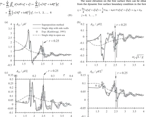
Fig. 9.Heave added mass and its components obtained by using superposition method.

-0.1

-0.05

0

0.05

0.1

0.15

1

1.5

2

2.5

3

3.5

4

-0.1

-0.05

0

0.05

0.1

0.15

0.2

0.25

0.3

0.35

1

1.5

2

2.5

3

3.5

4

0.1

0.2

0.3

0.4

-0.4

-0.3

-0.2

-0.1

0

0.1

0.2

1

1.5

2

2.5

3

3.5

4

-0.5

0

0.5

1

1.5

2

2.5

3

3.5

4

1

1.5

2

2.5

3

3.5

4

Superposition method Single ship with side walls Exp. (Kashiwagi, 1991) Single ship in open sea

33

/

A

ρ

V

A

35

/

ρ

VL

53

/

A

ρ

VL

2

55

/

A

ρ

VL

0.25

τ

=

0.25

τ

=

0.25

τ

=

0.25

τ

=

/

e

L g

ω

[image:7.595.46.548.316.720.2]

τ

whereζRjis the real part ofj-th model, andζIjis the imaginary part.

3.2. Validations

Before we carry out massive numerical calculations, a rigorous validation of the numerical programme should be conducted. Unfortunately, due to the complexities involved in the model test of two ships advancing in waves, only very limited model test data is available from the published resources.McTaggart et al. (2003)

andLi (2007)presented some experimental data of ship-to-ship with forward speed in waves based on their model tests carried out at the Institute for Marine Dynamics (IMD) in St. John's, Newfoundland. Similar work was also conducted by Ronæss (2002)and her model test was carried out at the Marine Tech-nology Centre in Trondheim, Norway. More recently,Xu and Dong (2013)carried out experimental tests to measure the wave loads and the free motions for a pair of side-by-side arranged ship models advancing with an identical speed in head regular waves. The validations of the present numerical programme MHydro against the model test results fromMcTaggart et al. (2003)and

Ronæss (2002)can be found inYuan et al. (2015a,2014a). In their validations, the heave and pitch RAOs of both ships were well predicted. However, they failed to predict the roll motion due to the viscus effects. In the present study, we are not going to make any efforts to calculate the motion RAOs. One of the reason has been demonstrated above as the viscus effect. Besides, the motion responses are not able to reflect the hydrodynamic interactions directly. For example, the motion responses are also determined by the mass and restoring force matrix, as well as the incident wave forces. And in most of the frequency range, the motion

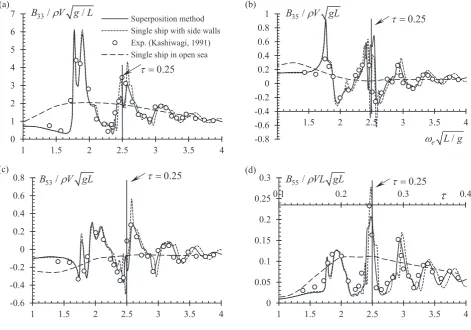
responses are dominated by these components rather than the radiation and diffraction forces. Therefore, in the present study, we are particularly interested in the hydrodynamic coef_ficients, which can directly reflect the hydrodynamic interaction. Without con-sideration of speed effects,Kashiwagi et al. (2005)published his model test results of the diffraction and radiation forces of a rec-tangular box and Wigley hull interacted in waves. We used his model test results to validate MHydro in zero speed case (Yuan et al., 2015a). Taking the forward into consideration, Kashiwagi and Ohkusu (1989,1991)conducted model test to investigate the ship and side wall interference. Kashiwagi (1993a, 1993b) also published some experimental results of the wave exciting forces and hydrodynamic coefficients about a catamaran. In the present study,Kashiwagi and Ohkusu (1991)model test results of side wall effects will be used here to validate the numerical programme. Based on the assumption that the ships involved in ship-to-ship problem are arranged side-by-side and the geometry and the speed of the ships are exactly the same, a single ship with side walls problem shown in Fig. 7 can be replaced by ship-to-ship problem shown inFig. 8. The existence of side wall 2 inFig. 7(a) is equivalent of replacing it with a mirror. The images of side wall 1 and Ship_a make the single ship with side walls problem exactly the same with ship-to-ship problem shown inFig. 8(b). Therefore, the superposition method used in the present study can be vali-dated through the model test of side wall effects conducted by Kashiwagi (1991).

[image:8.595.54.526.58.388.2]

The model used here is a half-immersed prolate spheroid of lengthL¼2.0 m and breadth B¼0.4 m. The model test was con-ducted in the towing tank (60 m length, 4 m breadth, 2.3 m in depth) of Nagasaki Institute of Applied Science. The model was

advancing at a Froude number Fn¼0.1 in the waterway of BT /L¼2.0, whereBTis the transverse distance between the ship and side wall. Two numerical simulations are performed by using MHydro. The first simulation adopts the same situation as that

used in the model test and the panel distribution and computa-tional domain of numerical model is shown inFig. 7(b). The cor-responding numerical results are referred as‘Single ship with side walls’hereafter. The second simulation is based on superposition method and two ships with side walls are modelled. The panel distribution and computational domain of numerical model is shown in Fig. 8(b), and the corresponding numerical results are

0

0.03

0.06

0.09

0.12

0.15

0

0.5

1

1.5

2

2.5

0

0.1

0.2

0.3

0.4

0.5

0.6

0

0.5

1

1.5

2

Superposition method

Single ship with side walls

Exp. (Kashiwagi, 1991)

Single ship in open sea

3

/

0 w

F

_{η ρ}

gA

5

/

0 w

F

_{η ρ}

gA L

/

L

λ

0.25

τ

=

0.25

τ

=

[image:9.595.43.288.58.390.2]

Fig. 12.Wave exciting forces of a half-immersed prolate spheroid ofB/L¼1/5 in waterway ofBT/L¼2.0 (Fn¼0.1). (a) Heave wave exciting force; and (b) pitch wave exciting moment.Awis the water plane area.

Table 1

Main dimensions of Wigley III hull.

Length,L(m) 3

Breadth,B(m) 0.3

Draught,D(m) 0.1875

Displacement,V(m3

) 0.078

Centre of rotation above base, KR (m) 0.1875 Centre of gravity above base,KG (m) 0.17 Radius of inertia for pitch,kyy(m) 0.75

Fig. 13.The computational domain of the numerical model. There are 12,090 pa-nels distributed on the entire computational domain: 600 on each body surface of Wigley hull, 9450 on the free surface and 1440 on the control surface. The com-putational domain is truncated at L upstream, 2L downstream, 0.5L sideways in the portside and 3L sideways in the starboard referred to Ship_a.

Table 2

Main parameters for each case.

Speedu0 (m/s)

Spacing d(m)

Staggered dis-tances(m)

Parameterτ Semi-wedge angleθ(°)

Case 1 1.22 1.2 0 0.88 30

Case 2 1.22 2.2 0 0.88 30

Case 3 1.22 2.2 1.5 0.38 30

Case 4 0.636 2.2 0 0.38 60

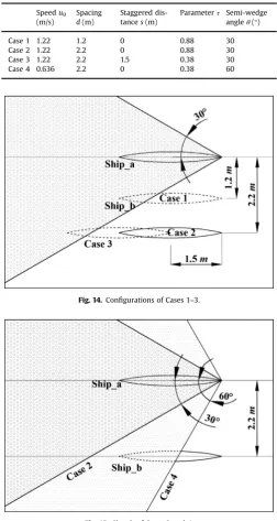
[image:9.595.310.563.77.551.2]

Fig. 14.Configurations of Cases 1–3.

[image:9.595.47.287.451.646.2]

Fig. 15.Sketch of Cases 2 and 4.

Table 3

Wave exciting forces on both ships of Cases 1–3.

Surge Sway Heave Roll Pitch Yaw

[image:9.595.312.562.592.659.2]

referred as‘Superposition method’. It should be noted that in both of the numerical simulations, the mesh size and the truncation of the free surface are consistent.

The hydrodynamic coefficients (for example, the added massA) obtained from the model tests and numerical simulation of single ship represent the total hydrodynamic coefficients of Ship_a di-rectly. However, the hydrodynamic coefficients of Ship_a obtained by using the superposition method consist of two components which can be written as A¼Aaa_þAab_{, whereA}aa _{represents the} added mass of Ship_a when Ship_a is oscillating while Ship_b is

fixed, andAabrepresents the added mass of Ship_a when Ship_a is

fixed while Ship_b is oscillating.Aaa_{can be obtained by solving the} boundary value problem from Eqs.(24)and(25), whileAab_{can be} obtained by solving the boundary value problem from Eqs.(26)

and(27). The heave added mass and its components are shown in

Fig. 9.Aab_{represents the effect of side wall 1 and it is the main} contribution of the negative added mass at certain frequencies.

Figs. 10and11show the hydrodynamic coef_ficients. Generally, the agreement between‘Superposition method’and‘Single ship with side walls’is satisfactory. Some discrepancies between‘ Su-perposition method’and‘Single ship with side walls’can be ob-served at high frequency range, which can be attributed to the numerical dispersion and damping (Kim et al., 2005) introduced by the constant panel method. The numerical dispersion and damping are mainly determined by the parameter

ε

(

ε

¼

λ

/dx, where

λ

is the wavelength anddx is the mesh size on the free surface). The numerical dispersion and damping are not noticeable at

ε

420. However, as

ε

o20, the numerical dispersion and damping become evident. In the present study, the wavelength

λ

is small at high frequency range. But as the unified mesh is applied, the parameter

ε

becomes very small. Therefore, the numerical dispersion and damping are inevitable. The numerical dispersion and damping becomes even more evident in ship-to-ship problem, since the free surface is larger than that in a narrow tank. The waves produced by Ship_a have to propagate a long distance until they strike Ship_b, and during this propagation, the numerical dispersion and damping occurs. However, in single ship with two side walls problem (the mesh size on the free surface is exactly the same as that in ship-to-ship problem), the free surface is smaller. The re_flected waves from the wall only travel a short distance, then they can strike the ship model. Therefore, the numerical dispersion and damping are not as obvious as that in ship-to-ship problem. The numerical dispersion and damping modify the wa-velength and amplitude during the propagation of the radiated waves (or reflected waves) and this is the main reason for the different phase and amplitude between the results obtained by two numerical methods at high frequency range. There are still some discrepancies that are found at 0.24o

τ

o0.27, which can be

attributed to the complicated waves trapped in the narrow gap between the side walls in the vicinity of the critical frequency. However, the general agreement between‘Superposition method’ and‘Single ship with side walls’is still satisfactory which indicates that the present method is capable to predict the hydrodynamic interactions between two ships with the same speed. As the parameter

τ

o0.25

(

ωe L g/ <2.5

)

, the hydrodynamic coefficients (radiation forces)fluctuate violently away from the open sea re-sults. As

τ

o0.25, the radiated waves from the mirrored spheroid (or the reflected waves from the side walls) can propagate to the domain where the spheroid is located and strike the spheroid. The agreement between the present calculations and experiments is very satisfactory even at parameter

τ

o0.25, which indicates the radiation condition included in the present numerical programme MHydro is capable to predict the hydrodynamic properties of the advancing ships even at parameter

τ

o0.25. As the parameter

τ

increases, the hydrodynamic coefficients gradually approach the open sea results and hydrodynamic interaction (or the side wall effects) trend to diminish.Fig. 12shows the wave exciting forces of a half-immersed prolate spheroid ofB/L¼1/5 in waterway ofBT /L¼2.0 (Fn¼0.1). Both of the heave force and pitch moment agree well with the experimental measurements. A very large spike can be observed at

λ

/L¼1.47, which corresponds to

τ

¼0.25. In the present study, we are particular interested in the range of

τ

40.272, where the semi-wedge angle

θ

exists and the minimum spacing can be determined by Eq.(20).

3.3. Case study

The validated numerical programme MHydro is used in this session to examine the reliability of the theoretical estimation of the minimum spacing. A series of case studies are designed here based on two identical Wigley III hulls advancing side by side in head waves with the same forward speed. Thus,

δ

in Eq. (20)is

fixed at 1, and then the dimensionless minimum spacing in Eq.

(20)is only determined by parameter

τ

. The main dimensions of Wigley III model is shown inTable 1. The computational domain and discretization of the boundaries is presented inFig. 13.

[image:10.595.32.283.80.130.2]

The incident wavelength to ship length ratio of

λ

/L¼1 in head sea corresponds to the critical conditions in ship design. In this case, the incident wave frequency

ω

0¼4.53 rad/s. Four typical cases, as shown inTable 2, are investigated in the present study to verify our assumption. These cases can be divided into two cate-gories, in order to make the comparisons conclusive. The _first category involves Cases 1–3. The basic principle for this category is that the forward speed isfixed at the same value atu0¼1.22 m/s. Therefore, according toFig. 4, the corresponding semi-wedge an-gle is 30°. But the positions of the ships are different. In Case 1, the spacing is 1.2 m, which means part of Ship_b is located in the wake region of Ship_a. In Case 2, the spacing is 2.2 m, which indicates that Ship_b is entirely located in the quiescent region of Ship_a. In Case 3, the spacing keeps the same as that in Case 2. But Ship_b is staggered at 1.5 m downstream. Thus, the stern of Ship_b will also be covered by Ship_a's wake. The configurations of thefirst cate-gory are depicted inFig. 14. The second category involves in Cases 2 and 4. The basic principle for this category is that the positions of

Table 4

Wave exciting forces on both ships of Cases 2 and 4.

Surge Sway Heave Roll Pitch Yaw

[image:10.595.35.556.684.746.2]

Single ship (u0¼0.636 m/s) 0.055 0.002 0.172 0.00013 0.277 0.002 Case 2 0.056 0.005 0.17 0.00027 0.279 0.005 Case 4 0.05 0.06 0.161 0.0024 0.263 0.045

Table 5

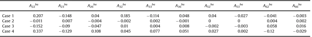
Added mass of Ship_b induced by the unit motion of Ship_a.

A22ba A23ba A26ba A32ba A33ba A36ba A52ba A53ba A62ba A66ba

Case 1 0.207 0.148 0.04 0.185 0.114 0.048 0.04 0.027 0.041 0.003

Case 2 0.011 0.007 0.004 0.002 0.002 0.001 0 0 0.004 0.002

Case 3 0.152 0.09 0.047 0.01 0.004 0.008 0.002 0.003 0.058 0.016

the ships in Case 4 are kept identical to that in Case 2, which has been described previously. The only difference between these two cases lies on the forward speed. In case 2, the forward speed is

fixed atu0¼1.22 m/s and the corresponding semi-wedge angle is 30°. Therefore, Ship_b would be entirely located in the quiescent region of Ship_a. But in Case 2, the forward speed isu0¼0.636 m/s. According toFig. 4, the corresponding semi-wedge angle is 60°, which means the major part of Ship_b would be located in Shi-p_a's wake. The sketch of Cases 2 and 4 is shown inFig. 15.

3.3.1. Wave exciting forces

The results of the wave exciting forces of Cases 1–3 are shown in Table 3. The results of the single ship are also included for comparison. The non-dimensionalisation for surge, sway and heave is made by using

η

0C33; the non-dimensionalisation for roll, pitch and yaw is made by using

η

0K0C55, where

η

0is the incident

wave amplitude, and C33and C55represent the restoring coeffi -cients in heave and pitch direction respectively. In Cases 1 and 2, the wave exciting forces on both ships are the same. But in Case 3, the staggered configuration violates the symmetrical property of theflowfield. As a result, the wave exciting forces of Ship_a and Ship_b are different, and they are listed individually inTable 3. In head wave condition, the best way to examine the hydrodynamic interactions is by calculating the sway, roll and yaw exciting forces. Theoretically, the sway, roll and yaw exciting forces of single ship must be zero due to the symmetrical characteristics of the incident

flow and body surface. But in numerical simulation, these forces

[image:11.595.42.562.80.138.2]

fluctuate around zero, which could attribute to the numerical er-rors. However, in Cases 1 and 3 (Ship_b), the wave exciting forces in sway, roll and yaw directions are very large. These forces on Ship_b are produced by the diffracted waves from Ship_a, since Ship_b in Cases 1 and 3 are partly located in the wake region of

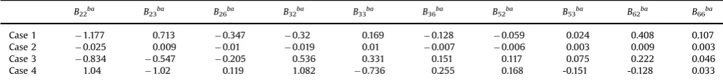
Table 6

Damping of Ship_b induced by the unit motion of Ship_a.

B22ba B23ba B26ba B32ba B33ba B36ba B52ba B53ba B62ba B66ba

Case 1 1.177 0.713 0.347 0.32 0.169 0.128 0.059 0.024 0.408 0.107

Case 2 0.025 0.009 0.01 0.019 0.01 0.007 0.006 0.003 0.009 0.003

Case 3 0.834 0.547 0.205 0.536 0.331 0.151 0.117 0.075 0.222 0.046

Case 4 1.04 1.02 0.119 1.082 0.736 0.255 0.168 -0.151 -0.128 0.033

Case 1

Case 2

Case 3

Case 4

R7

/ L:

-0.13 -0.10 -0.07 -0.05 -0.02 0.01

0.04

0.06

0.09

0.12

ζζ

[image:11.595.74.533.84.552.2]

Ship_a. But in Case 2, the wave exciting forces in these three di-rections are very small, which indicates that the diffracted waves from Ship_a could hardly influence theflowfield around Ship_b. Moreover, in Case 3, the wave exciting forces on Ship_a are almost identical to those of single ship case, which indicates that theflow

field around Ship_a could not be disturbed by the existence of Ship_b. The above findings are consistent with our assumption, and it can be concluded that in head waves, if both of the ships are located at each other's quiescent region, the diffracted interactions can be minimized.

The comparisons in Table 3 are based on the same forward speed (the same semi-wedge angle).Table 4presents some results with different forward speeds. Even though the configurations of Cases 2 and 4 are the same, the discrepancies between the cal-culated forces in sway, roll and yaw are signi_ficant. In Case 2, the diffracted waves produced by Ship_a are confined within a rela-tively smaller semi-wedge angle, and Ship_b is entirely located in the quiescent region. As a result, the wave exciting forces in sway, roll and yaw are very small. But as the forward speed decreases, the semi-angle becomes larger, and the quiescent region is shrunk. As a result, in Case 4, Ship_b will be partly covered by the dif-fracted wave field from Ship_a. Consequently, the wave exciting forces in sway, roll and yaw directions are significant, as shown in

Table 4. These results also coincide with our theoretical assumption.

3.3.2. Hydrodynamic coefficients

The added mass and damping of Ship_b induced by the unit motion of Ship_a are presented in Tables 5 and 6 respectively. These hydrodynamic coefficients reflect the influence from the radiated waves due to the existence of the other ship. The non-dimensionalisation for added mass with subscript of 22, 23, 32, and 33 is made by

ρ

V; the subscript of 26, 36, 52, 53 and 62 is made by

ρ

LV; the subscript of 66 is made by

ρ

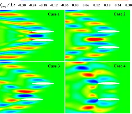
L2_{V. The} non-di-mensionalisation for damping with subscript of 22, 23, 32, and 33 is made byρV g L/ ; the subscript of 26, 36, 52, 53 and 62 is made by ρVL g L/ ; the subscript of 66 is made by ρVL2 g L/ _{. From the} results of Case 2, it can be found that the radiated waves produced by the unit motion of Ship_a could hardly in_fluence the hydro-dynamic properties of Ship_b. While in the other three cases, the hydrodynamic interaction on Ship_b is significant due to the dis-turbance of the radiated waves from Ship_a. The above conclu-sions are consistent with our theoretical assumption, which in-dicates that if the ship is located in the quiescent region of the other ship, the hydrodynamic interactions could be minimized.

3.3.3. Wave pattern

Figs. 16and17present the diffracted and radiated wave pat-terns for different cases. Because of the existence of Ship_a, the symmetrical property of theflowfield around Ship_b in Cases 1, 3 and 4 is violated. In these cases, the diffracted or radiated waves

Case 1

Case 2

Case 3

Case 4

R3

/ L:

-0.30 -0.24 -0.18 -0.12 -0.06 0.00 0.06 0.12 0.18 0.24 0.30

[image:12.595.77.510.76.451.2]

ζζ

produced by Ship_a could propagate to the body surface of Ship_b. But in Case 2, the nearfieldflow around Ship_b could hardly be disturbed by the existence of Ship_a. Even though the positions of the ships in Cases 2 and 4 are the same, the wave patterns in these two cases are different. In Case 2, the diffracted and radiated waves are confined within a relatively smaller semi-wedge angle. But in Case 4, due to the smaller value of

τ

, the waves are ex-panded to cover a larger fan-shape region. These observations coincide with our theoretical assumption. Fig. 18 gives the dif-fracted and radiated wave profiles at port and starboard of Ship_b. It can be found that in Cases 1, 3 and 4, the wave elevation at port and starboard of the stern region of Ship_b is different. This ex-plains why the sway, roll and yaw forces in these cases are very large. But in the fore region, the wave profiles tend to be identical to each other. It indicates that the waves produced by Ship_a could only propagate to the stern region of Ship_b in these cases. But in Case 2, the wave elevation at port and starboard of Ship_b is al-most the same. Only a very small discrepancy can be observed in the stern area. It indicates that the quiescent region calculated by the present stationary phase method is not absolutely calm water. Due to the continuity of the pressure distribution on the free surface, the wave elevation could not suddenly drop to zero when the waves propagate across the critical line (the line corresponds to the semi-wedge angle, which is used to divide the wake and quiescent regions, as shown inFig. 1). However, the wave elevation in the predicted quiescent region is not evident.

4. Hydrodynamic interaction diagram

It can be concluded from the numerical case study that the stationary phase method provides a general depiction of the wave propagation in the far-field. The critical line between the quiescent and wake region estimated from the far-field wave pattern can be

generally adopted to estimate whether the hydrodynamic inter-action is significant. However, the conclusion above is general and partial. The factors which determine the hydrodynamic interaction include several combinations of parameters: oscillation frequency, forward speed and transverse distance between two ships. Meanwhile the stationary phase method is not able to estimate accurately how much interactions are expected between two ships travelling in waves. Therefore, an accurate estimation of the cri-tical line is desired, which requires numerous simulations varying Froude number, frequency and transverse distance. A similar ap-proach which was adopted by Kashiwagi and Ohkusu (1991)to investigate the side-wall effects is introduced here to investigate ship-to-ship hydrodynamic interaction effects. In Kashiwagi and Ohkusu (1991) study, the side-wall effects are estimated by the difference between the hydrodynamic coefficients with side-wall and in the open sea. But in the present study, a more sophisticated parameter will be used to determine the hydrodynamic interac-tion effects. This parameter can be eitherAijaborAijaa. As discussed above, the superscript ‘ab’ directly reflect the interaction effect from the existence of the other ship. The coefficients with super-script‘ab’are referred as the external-induced components while the superscript‘aa’denotes the self-induced ones. For single ship case, the self-induced components do not exist.

Fig. 19shows the external-induced components of the hydro-dynamic coefficients, which is non-dimensionlized by the single ship results. Strictly speaking, there should be 36 independent components of each set of external-induced hydrodynamic

coef-ficients if the two ships are not identical. Even in case of two identical ships, there are 21 independent components contained in the external-induced hydrodynamic coefficient matrix (Aijab=Ajiab, i¼1,2,…,6;j¼1,2,…,6). In order tofind the region where there is no hydrodynamic interaction, all of these components should be zero. In the numerical calculation, due to the numerical error,

-0.4

-0.2

0

0.2

0.4

0.6

0.8

1

-0.5

-0.3

-0.1

0.1

0.3

0.5

Case 1

ζR3/ η0

ζR7/ η0

Portside

Starboard

ζ / η

₀

-0.3

-0.2

-0.1

0

0.1

0.2

0.3

0.4

-0.5

-0.3

-0.1

0.1

0.3

0.5

Case 2

ζR7/ η0

ζR3/ η0

ζ / η

₀

-0.4

-0.3

-0.2

-0.1

0

0.1

0.2

0.3

-0.5

-0.3

-0.1

0.1

0.3

0.5

Case 3

ζR7/ η0

ζR3/ η0

ζ / η

₀

-0.6

-0.4

-0.2

0

0.2

0.4

0.6

-0.5

-0.3

-0.1

0.1

0.3

0.5

Case 4

ζR3/ η0

ζR7/ η0

X / L

[image:13.595.64.536.58.360.2]

ζ / η

₀

these components are impossible to be zero, even for single vessel in open sea. Therefore, we have to set a permissible error. If the calculation values are bellow this permissible error, no hydro-dynamic interaction is expected. In the present study, the per-missible error is defined as 0.2%. Coincidently, the calculated re-sults are quite consistent and convergent, even though the dif-ferent componentsfluctuate with different amplitudes. Therefore, we only display four typical components inFig. 19. FromFig. 5we canfind the assumptive critical

τ

¼0.521 estimated from the

far-field asymptotic wave pattern at d/L¼1. Theoretically, no

hydrodynamic interactions are expected at

τ

40.521. However, the numerical calculations presented in Fig. 19 shows a significant hydrodynamic interaction effect at

τ

¼0.521, and some compo-nents even experience an increasing trend at

τ

40.521. The hy-drodynamic interaction effects gradually diminish and the ex-ternal-induced hydrodynamic coefficients are convergent to the permissible error. AtFn¼0.15, the curves are convergent to the permissible error at

τ

¼0.677. As the Froude number increases, the convergent point is extended to

τ

¼0.773 atFn¼0.2 and

τ

¼0.909 atFn¼0.25. It indicates as the Froude number increases, the actual quiescent region will shrink.

FromFig. 19it can be found that for any given Froude number, we can always_find a critical frequency. Therefore, we can de-termine the critical lines showing the existence of the hydro-dynamic interaction effects as a function of Froude number, fre-quency and transverse distance. Results are shown in Fig. 20, wherex-axis is the g L/ /ωe=Fn/τ,y-axis isFn. The ratio ofytoxis parameter

τ

. In the present numerical calculation, as the two ships are in the same length (

δ

¼1), for a given value ofd/L, the critical parameter

τ

is unique. Therefore, the dashed lines inFig. 20are linear and they represent the critical line estimated from the asymptotic far-field wave theory. The solid curves are the calcu-lated critical lines, which approach the dotted lines at high fre-quency, where the wavelength is relatively small compared to the transverse distance between two ships and the theoretical esti-mation is valid. As the encounter frequency decreases, the dis-crepancies become evident and the range of hydrodynamic inter-action effects expands. The difference between the dashed lines and solid curves is due to the effect of the near-field non-radiation local waves in the vicinity of the ships.

[image:14.595.36.280.56.579.2]

The permissible error can be various, for example, 1%. From

Fig. 19it can be found the critical parameter

τ

shifts to a smaller value and the discrepancies between the dashed lines and solid curves become small. However, the selection of the permissible error must be very careful. It should not be very large, for example 5%, otherwise the curves of the hydrodynamic coefficients will be subject to fluctuations before they tend to convergent. On the other hand, the results of different components will be incon-sistent and individual diagrams are required.

5. Conclusions

In this paper, we presented a method based on Havelock form of the Green function to predict the far field wave pattern

-20%

-10%

0%

10%

20%

3

3.4

3.8

4.2

4.6

0.45

0.49

0.53

0.57

0.61

0.65

0.69

Assumptive critical line between quiescent and wake region

Calculated critical line

0.4

0.5

0.6

0.7

0.8

-20%

-10%

0%

10%

20%

2

2.5

3

3.5

4

Assumptive critical line

Calculated critical line

e

L

/

g

-15%

-5%

5%

15%

25%

1.6

1.9

2.2

2.5

2.8

3.1

3.4

3.7

4

0.4

0.5

0.6

0.7

0.8

0.9

1

Assumptive critical line

Calculated critical line

Fig. 19.External-induced hydrodynamic coefficients of identical Wigley hulls atd/ L¼1. (a)Fn¼0.15; (b)Fn¼0.2; (c)Fn¼0.25. The results are non-dimensionlized by the corresponding values of single vessel in open sea, and the superscript‘s’ofA_ijs

[image:14.595.305.551.60.234.2]

orBijsdenotes the single vessel results.