Deep residual neural network for EMI event classification using bispectrum representations

Deep Residual Neural Network for EMI Event

Classification Using Bispectrum Representations

Imene Mitiche

, Mark David Jenkins

, Philip Boreham

Alan Nesbitt

, Brian G. Stewart

and Gordon Morison

∗ _{School of Engineering and Built Environment}

Glasgow Caledonian University, Glasgow, United Kingdom † _{Institute of Energy and Environment}

University of Strathclyde, Glasgow, United Kingdom ‡_{Innovation Centre for Online Systems}

Bere Regis, United Kingdom

Abstract—This paper presents a novel method for condition monitoring of High Voltage (HV) power plant equipment through analysis of discharge signals. These discharge signals are mea-sured using the Electromagnetic Interference (EMI) method and processed using third order Higher-Order Statistics (HOS) to obtain a Bispectrum representation. By mapping the time-domain signal to a Bispectrum image representations the problem can be approached as an image classification task. This allows for the novel application of a Deep Residual Neural Network (ResNet) to the classification of HV discharge signals. The network is trained on signals into 9 classes and achieves high classification accuracy in each category, improving upon our previous work on this task.

I. INTRODUCTION

Electromagnetic Interference (EMI) measurement is a method utilised for Partial Discharge (PD) detection in High-Voltage (HV) systems [1]. PD is an electrical discharge that occurs due to failure in an insulation medium [2], which if neglected, could cause equipment breakdown resulting high maintenance or replacement costs. EMI diagnosis involves EMI signals measurement followed by experts analysis in order to identify presence of faults or insulation degradation in the HV equipment including cables, generators, motors, transformers etc. [3]. This technique captures PD as well as other discharge sources such as Corona, Arcing etc. The current EMI diagnosis method is manual, this means larger time spent on data acquisition and analysis is unavoidable, which implies high remuneration. Furthermore, this method is not practical for continuous monitoring. There may also be a lack in trained and experienced EMI experts and interpretation of EMI data could be challenging [4].

A proposed solution in this paper is to develop an auto-matic fault diagnosis model based on state-of-the-art signal processing techniques. A literature review on PD detection and classification techniques is provided in [5]–[7]. The summary of these papers includes a comparison of PD measurement methods and covers a large number of feature extraction and classification techniques that were proposed for PD

This paper is structured as follows. Section 2 defines the feature extraction and classification algorithms employed in this work. Section 3 introduces the experimental set-up with a brief description on EMI data collection. Section 4 presents the classification results in terms of classification accuracy and confusion matrices. Finally, Section 5 draws conclusions from this research with future plans.

II. FEATURE EXTRACTION AND CLASSIFICATION ALGORITHMS DESCRIPTION

A. Bispectrum Analysis

In time-domain HOS analysis, the first-order moment of a discrete signalx[n];n= 1, ..., Nis the meanµand its second-order moment is the varianceσ2_{, both are defined in Equation}

1 and 2 respectively.

µ=E(x[n]). (1)

σ2=E(x[n]x[n+τ1]). (2)

The third-order moment of the signal is defined as:

γ=E(x[n]x[n+τ1]x[n+τ2]). (3)

whereτ1andτ1are time lags. Assuming that the signalx[n]

is zero mean, then the second- and third- order cumulants are equal to the respective moments [16]. In frequency-domain definition, the third-order cumulant spectrum, known as the Bispectrum, is the Fourier Transform (FT) of the third-order moment which can be defined as:

B(f1, f2) = N

X

τ1=1

N

X

τ2=1

N

X

n=1

x[n]x[n+τ1]x[n+τ2]

·e−j2π·(f1τ1+f2τ2)_{. (4)}

Letn+τ1=mandn+τ2=k, by rewriting Equation 4 and

splitting the exponent, Bispectrum can be reformulated as:

B(f1, f2) ={ N

X

m=1

x[m]e−j2πf1m_{} · {}

N

X

k=1

x[k]e−j2πf2k_}

· { N

X

n=1

x[n]e+j2π(f1+f2)n_}=X(f

1)X(f2)X∗(f1+f2). (5)

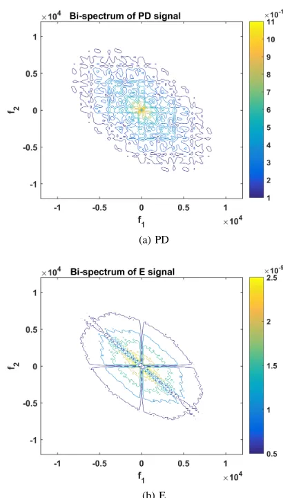
where X(f) is the FT and X∗(f)is the complex conjugate of X(f). The Bispectrum is a complex measure that contains both magnitude and phase information, unlike the power spec-trum. The Bispectrum reveals its content in two independent frequenciesf1andf2. Figure 1 shows an example Bispectrum

contour map of PD and E signals. The time domain of the two signals is provided in Figure 2. It is observed that both time signals have similar content in terms of pulses which may be challenging for their classification. However, the Bispectrum of these two signals reveals a unique signature for each signal type.

(a) PD

(b) E

Fig. 1. Bispectrum image of PD and E events

B. Deep Residual Network

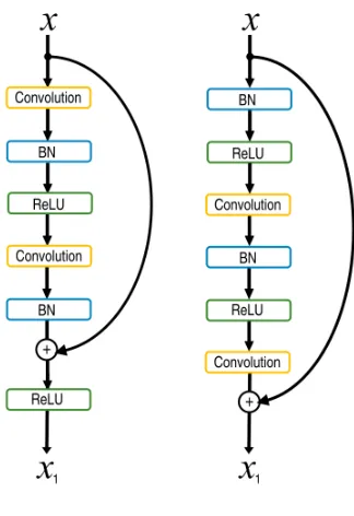
The application of Deep Residual Networks (ResNets) [17] to the image classification problem has become very popular since the use of a very deep networks to achieve state-of-the-art results on challenges such as ImageNet [18]. A residual network differs from a standard Convolutional Neural Network (CNN) through the implementation of identity skip connec-tions or shortcuts. These shortcut connecconnec-tions have been shown to reduce the potential for vanishing/exploding gradients [19] and reduce training loss and error [17]. To exploit the power of ResNet architectures in image classification, this work attempts to use the image representation of the Bispectrum of the time domain signal for classification. The residual network utilised in this work is based on the 34 layer ResNet from [17]. Figure 3 shows two possible configurations of what will be referred to as residual blocks. These blocks consist of a combination of convolutions, Batch Normalisations (BN) and ReLU Activations [20] as well as a shortcut connection with associated addition. These residual blocks are used to build the complete ResNet-34 architecture as detailed in Table I.

(a) PD time-series

(b) E time-series

Fig. 2. Time-domain signal of PD and E events

(a) Standard Configuration (b) Pre-Activation

Fig. 3. Residual Block Configurations

TABLE I

STRUCTURE OF THERESNET-34 ARCHITECTURE WHERE ARESIDUAL BLOCK CAN BE SUBSTITUTED FOR ANY SUITABLE BLOCK

CONFIGURATION SUCH AS THOSE INFIGURE3

Layer Kernel Depth Stride Operation

1 7x7 64 2 Conv

2 3x3 - 1 MaxPool

3 3x3 64 1 Residual Block x 3 4 3x3 128 1 Residual Block x 4 5 3x3 256 1 Residual Block x 6 6 3x3 512 1 Residual Block x 3 7 Average Pool, Fully Connected, SoftMax

upon the original sturcture of the residual blocks by utilising a pre-activation configuration. By applying the BN and ReLU functions before the convolutions, the pre-activation residual block structure (shown in Figure 3b) has been shown to reduce test error as well as prevent overtraining of the model. This is the residual block structure implemented in this work with learning rate of 0.01.

III. EMIDATA ACQUISITION AND EXPERIMENTAL SET-UP

EMI measurement follows the method specified in the CISPR 16 (Committee International Special des Perturbations Radioelectriques) Standard [22], which involves a quasi-peak detector with various filter bandwidths over a frequency span. Examples include the B filter which operates over 150kHz-30MHz, with a 6dB bandwidth of 9kHz, and the C filter from 30-300MHz with a 6dB bandwidth of 120kHz. The quasi-peak detector has a sampling time of 1 second per selected frequency and it is fast enough to capture the discharges intensity [23]. Further details on EMI measured frequency spectrum can be found in [3], [23], [24]. EMI time resolved signals can be retrieved from the frequencies of interest in the spectrum. The signals are subsequently analysed by EMI experts with the aim of identifying the presence of any discharge source [25], based on past accumulated experience of fault diagnosis and forensic confirmation. The signals in this paper were measured during the assets’ operation by means of High Frequency Current Transformer (HFCT) which is connected around the neutral earth cable of the asset. The signals are recorded at a sampling rate of 24kHz on a PD Surveyor 200 (PDS200) instrument which operates following the CISPR16 standard for EMI filter types. The PDS200 is able to detect and analyse Radio Frequency Interference (RFI) in addition to EMI radiations in the lower frequency range [50kHz-1GHz].

Fig. 4. Time series Classification approach using Bi-Spectrum image feature and ResNet-34 Neural Network

Fig. 5. Overall experimental set-up, from EMI data measurement, EMI expert analysis and labelling, to the proposed classification approach

of 9 events (classes) known as Arcing (A), Corona (C), Data Modulation (DM), Exciter (E), PD, Process Noise (PN), Random Noise (RN), minor PD (mPD) and micro Sparking (mS). The second stage involves the application of signal processing techniques including feature extraction and the ResNet-34 to the measured and labelled EMI signals. Here, the magnitude of the Bispectrum is extracted from each signal to obtain relevant information. Pre-processing such as image scaling is also performed in order to aid the learning process. The network is trained on 14,000, validated on 2000 and tested on 2000 BiSpectrum images from 9 classes. The model is implemented using Keras and Tensorflow and training takes approximately one hour on an NVIDIA Titan Xp GPU with 12GB RAM.

IV. CLASSIFICATION RESULTS

Experiment results are presented in terms of classification accuracy as well as confusion matrix, since 9 classes are presented to the developed model. Table II presents results from each run output of a 10 validation folds and the average performance. It is observed that the highest classification

ac-TABLE II

CLASSIFICATION ACCURACY RESULTS

Run No. Acc. %

1 97.23

2 95.10

3 97.23

4 89.82

5 86.24

6 93.33

7 89.14

8 92.81

9 85.55

10 95.97 Average acc. % 92.24

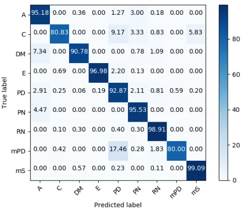
curacy was achieved in the first and third runs with 97.23%, as underlined in the table. Whereas, the lowest accuracy obtained is 85.55%. Yet, it has been found that the overall performance is consistent and the average accuracy surpasses the 90% score which is excellent for a classification of 9 different classes. In order to better understand the obtained performance results, the average confusion matrix is illustrated in Figure 6. The major misclassification is seen between mPD and PD with 17.46% of mPD being classified as PD. This could be because mPD is a subset fault type of PD. In fact mPD represents the occurrence of PD at lower repetition rate and discharge level which makes their classification ambiguous.

V. CONCLUSION

Fig. 6. Average Confusion Matrix calculated over the 10 validation folds

REFERENCES

[1] J. E. Timperley, D. Buchanan, and J. M. Vallejo, “Electric generation condition assessment with electromagnetic interference analysis,”IEEE Transactions on Industry Applications, vol. PP, pp. 1–1, 2017. [2] F. Kreuger, Industrial High Voltage: 4. Coordinating, 5. Testing, 6.

Measuring. Delft University Press, 1992.

[3] J. E. Timperley and J. M. Vallejo, “Condition assessment of electrical apparatus with emi diagnostics,”IEEE Transactions on Industry Appli-cations, vol. 53, pp. 693–699, 2017.

[4] C. V. Maughan, “Electromagnetic interference (emi) testing of electrical equipment,” in2011 Electrical Insulation Conference (EIC)., 2011, pp. 340–344.

[5] W. J. K. Raymond, H. A. Illias, A. H. A. Bakar, and H. Mokhlis, “Partial discharge classifications: Review of recent progress,” Measurement, vol. 68, pp. 164 – 181, 2015.

[6] M. Wu, H. Cao, J. Cao, H. L. Nguyen, J. B. Gomes, and S. P. Krishnaswamy, “An overview of state-of-the-art partial discharge anal-ysis techniques for condition monitoring,” IEEE Electrical Insulation Magazine, vol. 31, pp. 22–35, 2015.

[7] M. Mondal and G. Kumbhar, “Detection, measurement, and classifica-tion of partial discharge in a power transformer: Methods, trends, and future research,”IETE Technical Review, vol. 0, pp. 1–11, 2017. [8] I. Mitiche, G. Morison, A. Nesbitt, P. Boreham, and B. G. Stewart,

“Classification of partial discharge emi conditions using permutation entropy-based features,” in 2017 25th European Signal Processing Conference (EUSIPCO), 2017, pp. 1375–1379.

[9] I. Mitiche, G. Morison, A. Nesbitt, M. Hughes-Narborough, P. Boreham, and B. G. Stewart, “Classification of partial discharge signals by combining adaptive local iterative filtering and entropy features,” in2017 IEEE Conference on Electrical Insulation and Dielectric Phenomena., 2017, pp. 335–338.

[10] S. Li and Y. Liu, “Feature extraction of lung sounds based on bispec-trum analysis,” in2010 Third International Symposium on Information Processing, 2010, pp. 393–397.

[11] A. Lanat, G. Valenza, C. Mancuso, and E. Scilingo, “Robust multiple cardiac arrhythmia detection through bispectrum analysis,”Expert Sys-tems with Applications, vol. 38, pp. 6798 – 6804, 2011.

[12] N. Kumar, K. Khaund, and S. M. Hazarika, “Bispectral analysis of eeg for emotion recognition,”Procedia Computer Science, vol. 84, pp. 31 – 35, 2016, proceeding of the Seventh International Conference on Intelligent Human Computer Interaction (IHCI 2015).

[13] D. Bhalke, C. R. Rao, and D. Bormane, “Hybridisation of mel frequency cepstral coefficient and higher order spectral features for musical

instru-ments classification,” Archives of Acoustics, vol. 41, pp. 427 – 436, 2016.

[14] D. G. Bhalke, C. B. R. Rao, and D. S. Bormane, “Musical instrument classification using higher order spectra,” in2014 International Confer-ence on Signal Processing and Integrated Networks (SPIN), 2014, pp. 40–45.

[15] F. A. H. Jinying, S. B. P. Hongxia, and T. C. B. Shihua, “Bispectrum entropy feature extraction and its application for fault diagnosis of gearbox,” inInternational Conference on Fuzzy Systems, 2010, pp. 1–6. [16] K. C. Chua, V. Chandran, U. R. Acharya, and C. M. Lim, “Application of higher order statistics/spectra in biomedical signalsa review,”Medical Engineering and Physics, vol. 32, pp. 679 – 689, 2010.

[17] K. He, X. Zhang, S. Ren, and J. Sun, “Deep residual learning for image recognition,” inProceedings of the IEEE conference on computer vision and pattern recognition, 2016, pp. 770–778.

[18] O. Russakovsky, J. Deng, H. Su, J. Krause, S. Satheesh, S. Ma, Z. Huang, A. Karpathy, A. Khosla, M. Bernsteinet al., “Imagenet large scale visual recognition challenge,”International Journal of Computer Vision, vol. 115, pp. 211–252, 2015.

[19] C. Szegedy, W. Liu, Y. Jia, P. Sermanet, S. Reed, D. Anguelov, D. Erhan, V. Vanhoucke, A. Rabinovichet al., “Going deeper with convolutions,” in2015 IEEE Conference on Computer Vision and Pattern Recognition (CVPR), 2015, pp. 1–9.

[20] V. Nair and G. E. Hinton, “Rectified linear units improve restricted boltz-mann machines,” inProceedings of the 27th international conference on machine learning (ICML-10), 2010, pp. 807–814.

[21] K. He, X. Zhang, S. Ren, and J. Sun, “Identity mappings in deep residual networks,” in European Conference on Computer Vision. Springer, 2016, pp. 630–645.

[22] CISPR/CIS/A - Radio-interference measurements and statistical meth-ods, EMC 33.100.10 - Emission, 2015.

[23] J. E. Timperley, “Comparison of pda and emi diagnostic measurements [for machine insulation],” inConference Record of the the 2002 IEEE International Symposium on Electrical Insulation (Cat. No.02CH37316), 2002, pp. 575–578.

[24] J. E. Timperley, J. M. Vallejo, and A. Nesbitt, “Trending of emi data over years and overnight,” in 2014 IEEE Electrical Insulation Conference (EIC), Philadelphia, USA, 2014, pp. 176–179.

[25] J. E. Timperley, “Audio spectrum analysis of emi patterns,” in 2007 Electrical Insulation Conference and Electrical Manufacturing Expo, Nashville, USA, 2007, pp. 39–41.