A Theoretical Approach to Molecular Design: Planar-Tetracoordinate Carbon

Theoretical Methods

2.1 Introduction 51

2.2 Basic Concepts 53

2.2.1 The Schrödinger Equation 53

2.2.2 The Born–Oppenheimer Approximation 54 2.2.3 Orbitals and the Basis Set Expansion 55

2.2.4 The Variational Theorem 56

2.3 Single-Determinant Methods 56

2.3.1 Hartree–Fock (HF) Theory 56

2.3.2 Electron Correlation 58

2.4 Multireference Methods 64

2.4.1 Active Space Considerations 64

2.4.2 Including Dynamic Correlation 65

2.5 Basis Sets 66

2.5.1 Split-Valence and Mixed Basis Sets 67 2.5.2 Polarization and Diffuse Functions 68

2.5.3 Pople Basis Sets 68

2.5.4 Correlation-Consistent Basis Sets 69

2.6 Hierarchy of Ab Initio Methods 70

2.7 Density Functional Theory 71

2.7.1 Kohn–Sham Theory 71

2.7.2 Functionals 72

2.8 Semi-empirical Procedures 74

2.9 Potential Energy Surfaces 75

2.9.1 Geometry Optimization 75

2.9.2 Normal Mode Analysis 76

2.9.3 Zero-Point Energies 76

2.10 Molecular Properties 77

2.10.1 Symmetry 77

2.10.2 Strain Energies 77

2.10.3 Heats of Formation 79

2.10.4 Proton Affinities 79

2.10.5 Ionization Energies 80

2.11 Computational Resources 80

2.11.1 Software 80

2.11.2 Hardware 80

2.11.3 Resource Usage 81

2.12 Notation and Abbreviations 84

2.13 Units 86

References 86

2.1 Introduction

Computational quantum chemistry has become an invaluable tool for the

con-sidering individual molecules as a group of particles that can be treated using the

equa-tions of quantum mechanics (which treat particles like waves). Its value was given the

ultimate accolade in 1998 when the Nobel Prize in Chemistry was awarded to “John A.

Pople for his development of computational methods for use in quantum chemistry” and

“Walter Kohn for his development of the density functional theory”.

In practice, any natural system interacts with its environment to some extent and so

any complete solution is effectively infinite and clearly intractable. Fortunately, it is

possible to simplify most systems by limiting them to some natural boundary. For the

chemist, and in particular the organic chemist, this boundary falls naturally at the

molec-ular level. The natural boundary in this case is a consequence of the large difference

between the strength of covalent bonds and intermolecular forces.† As a result, chemical

systems which involve either individual molecules or a small number of interacting

mol-ecules (a chemical reaction) can be readily treated using quantum mechanical

tech-niques. The systems that have been examined in this work (saturated hydrocarbon cage

compounds) all fall into the category of well-bounded covalent molecules and are thus

well-suited to study by the computational techniques outlined in this chapter.

However, it turns out that the resulting equations are insoluble for all but the very

simplest systems, i.e. exact solutions are available for systems of only one or two

parti-cles.1 To solve the resulting equations for all other systems requires the use of various

approximations, and in most cases the use of computers to calculate the solution. The

so-called ab initio methods‡ achieve this using only the laws of quantum mechanics, along with the fundamental constants of nature, e.g. the speed of light and Planck’s

con-stant, and various rigorously defined mathematical approximations.§ The methods

known as semi-empirical use a number of empirically derived parameters for each of the

atoms, which are determined by fitting calculated results to experimental data. This

†

This is obviously not the case in all situations. Solvation has the effect of blurring the boundary between a discrete molecule and its environment. However, rather than attempting to treat the entire system as one large quantum system, ways are being developed to treat the boundary and apply the effects of the environ-ment as a continuum or other non-quantum system.

‡

The term “ab initio” was first used in this context by Emeritus Professor David Craig of the Australian National University.6

§

enables more drastic simplification of the quantum mechanical equations but in doing so

introduces both some degree of prejudice towards the systems used in the

parametriza-tion, and an incompleteness or inflexibility in the treatment that has been found in

prac-tise to sometimes lead to poor results outside the ‘test set’ used for the parametrization.

Because the complexity and the size of the problem, and as a result, the time to

compute a solution, increases rapidly with the size of the system, increasing levels of

approximation are required to treat ever larger systems. However, the steady advance in

computer technology, which is well described by Moore’s Law,† has meant that ever

larger molecules can be investigated by the methods described hereafter.

This chapter presents a brief overview of the theoretical methods used in this thesis.

More detailed discussions of these and other methods can be found elsewhere.1–4

2.2 Basic Concepts

2.2.1 The Schrödinger Equation

The state of almost any system can be described by the time-independent

Schrödinger equation,5 _{which is most simply written as,}

HΨ = EΨ (2-1)

where H is the Hamiltonian, a differential operator representing the total energy

(described below), Ψ is the wavefunction and E is the total energy of the system. The Hamiltonian operator (H) can be divided into two components, corresponding to the

kinetic and potential energy, i.e.

H = T + V (2-2)

where T and V are the kinetic and potential energy operators, respectively.

For a molecular system, the Hamiltonian operator can be written in atomic units as

†

follows,3

(2-3)

where i and j represent the ith and jth electrons, a and b are the ath and bth nuclei, M_a is the mass of the ath nucleus relative to that of an electron, Z_a is the charge on nucleus a, and r_xy is the distance between the particles x and y. The first two terms represent the kinetic energy of the electrons and nuclei, respectively, while the remainder represent

the potential energy.

2.2.2 The Born–Oppenheimer Approximation

The complexity of Equation 2-3, and hence the difficulty of determining a solution,

can be reduced somewhat by employing a simple approximation, known as the

Born–Oppenheimer (or adiabatic) approximation.7 Since the nuclei are much heavier

than the electrons, it is reasonable to suggest that the electrons can adjust rapidly to any

change of the nuclear configuration, i.e. we assume that the electronic distribution

depends on the instantaneous positions of the nuclei and not on their velocities. This

allows separation of the Hamiltonian (Equation 2-3) into nuclear and electronic

compo-nents, which allows calculation of the energy (an effective electronic energy) at fixed

nuclear configurations. The electronic Hamiltonian is shown in Equation 2-4 below,

(2-4)

The hypersurface describing the variation of energy with nuclear position for a given

electronic state is known as the potential energy surface (PES).

Although the Born–Oppenheimer approximation allows for considerable

simplifi-cation, the resulting equations still have no analytic solutions except for one-electron

systems (e.g. H₂+). In order to make these methods applicable to systems of chemical

interest, approximations for treating the electron many-body problem must also be

included.

H = − ∇i

2

2

i=1 N_e

∑

2M_a

a=1 N_n

∑

r_ia

a=1 N_n

∑

N_e

∑

r_ij +

Z_aZ_b r_ab

b>a N_n

∑

N_n

∑

N_e

∑

∑

H= − ∇i

2

2

i=1 N_e

∑

r_ia

a=1 N_n

∑

N_e

∑

r_ij

j>i N_e

∑

2.2.3 Orbitals and the Basis Set Expansion

2.2.3.1 The Molecular Orbital Approximation

The essence of the molecular orbital approach is to further simplify the Schrödinger

equation (Equation 2-1) by assuming that the motion of each electron is independent.

Although this does not give an accurate description of the electron it serves as a useful

approximation and the correlation of motions between electrons can be dealt with in

other ways (as will be seen later). The wavefunction of the system can then be

expressed as a product of one-electron wavefunctions, referred to as spin-orbitals. Each

spin-orbital χ, is the product of a spatial function (ψ), which is dependent on the posi-tion of the electron (and whose square gives the probability distribuposi-tion of the electron

in space), and a spin function, indicating the spin state of the electron.

Because electrons are fermions the total electronic wavefunction must be

antisym-metric (change sign) with respect to interchange of any two electron coordinates. A

simple product of spin-orbitals is not adequate. The Pauli exclusion principle, which

states that no two electrons can have all quantum numbers equal, is a direct consequence

of the antisymmetry requirement. A wavefunction that does have the antisymmetry

requirement and which obeys the Pauli principle can be formed from the determinant of

the n-electron spin-orbital matrix,

(2-5)

where χ_i(j) indicates electron j occupying the spin orbital χ_i and the prefactor is a nor-malization constant. Expansion leads to a sum of products of spin orbitals. This

expres-sion is commonly referred to as a Slater determinant.8

2.2.3.2 Basis Set Expansions

In practice, the spatial component of a spin-orbital is expanded in terms of a finite

set of one-electron basis functions (φ_µ) which are usually atom centered. The molecular

Ψ = 1

n!

χ1(1) χ2(1) L χn(1) χ1(2) χ2(2) L χn(2)

M M M

orbitals can now be written as,

(2-6)

where c_µi are the molecular orbital expansion coefficients, which represent the contribu-tions from each of the basis funccontribu-tions to the molecular orbital. When the atomic orbitals

of the substituent atoms are used as basis functions, the method is known as a linear

combination of atomic orbitals (LCAO).

2.2.4 The Variational Theorem

The variational theorem1–4 states that the energy (E_approx) of an approximate

wave-function (Ψ_approx) is an upper bound to the exact energy (E_exact), i.e.

(2-7)

This allows an iterative approach to optimizing the molecular orbital coefficients (c_µi) in order to obtain the minimum total energy. This will give the best wavefunction possible

within the constraints of the approximations used. Methods that calculate the energy

utilizing Equation 2-7 are said to be variational.

2.3 Single-Determinant Methods

2.3.1 Hartree–Fock (HF) Theory

Applying the variational theorem (Equation 2-7) to an approximate N-electron

wavefunction formed by the methods described above gives the Roothaan–Hall

equa-tions,9

(2-8)

where F_µv is the Fock matrix, ε_i is the energy of the molecular orbital ψ_i and S_µv is the overlap matrix. Since the Fock matrix F_µvis itself dependent on the orbital coefficients

c_µi,these equations are not linear and must be solved iteratively until convergence of the energy and the orbital coefficients is achieved.

ψi = cµiφµ

µ =1 N

∑

E_approx = Ψapprox

*

HΨ_approx dτ

∫

Ψ_approx* _Ψ

approx dτ

∫

c_µi µ =1

N

This approach was first proposed by Hartree10 and Fock11 and is referred to as

Har-tree–Fock (HF) theory. Because the molecular orbitals are derived from their own

effec-tive potential, this technique is also often referred to as self-consistent-field (SCF)

the-ory (although it is one of many procedures that make use of such an iterative approach

to achieving self-consistency in the electronic probability distribution).

If the Roothaan–Hall equations are formulated in such a way that each spatial

molecular orbital should contain two electrons, one of α and one of β spin, the resulting wavefunction is known as a restricted Hartree–Fock (RHF) solution. This procedure

works well for most ground-state molecules where the electronic configuration is

well-described as a closed-shell singlet state. The majority of the calculations conducted in

this work fall into this category. It has been necessary to consider open-shell states in a

number of cases.† The Roothaan–Hall equations can be reformulated to remove the

restriction that all spatial molecular orbitals be doubly-occupied. The most direct way

of doing this, known as the unrestricted Hartree–Fock (UHF) method, defines two sets

of Roothaan–Hall equations (the Pople–Nesbet equations12), one describing the α -elec-trons and one for the β-electrons. Allowing the spatial components of the spin-orbitals to vary, including those that are doubly-occupied, makes it possible for unpaired spins to

interact differently with the α- and β-electrons in the ‘doubly-occupied’ orbitals, even though this is ‘unphysical’. When this occurs, the resulting wavefunction is no longer

an eigenfunction of <S2> (the expectation value of the spin-squared operator) because it is effectively including contributions from other high-lying spin states of the molecule.

The added flexibility in the density distribution of the electron can also be seen as a

weak form of electron correlation (see Section 2.3.2 on page 58). There is another

for-mulation known as restricted open-shell Hartree–Fock (ROHF) which we have not used

in this work but which is well described elsewhere.1–4

There are two fundamental limitations to the Hartree–Fock method. In the first

place, it ignores relativistic effects, but since these effects are only important for heavier

atoms (e.g transition metals), they need not concern us here. The second, more serious

limitation, is its neglect of electron correlation. Methods for including electron

correla-†

tion are discussed below.

2.3.2 Electron Correlation

As has been seen, the HF equations replace the real electron–electron interaction

with an average interaction in which each electron ‘sees’ only the ‘field’ generated by

the other electrons. This does not account for direct interactions between pairs of

elec-trons. This pair-wise electron interaction is termed electron correlation and is often

sep-arated into Coulomb and Fermi correlation terms, which correspond to opposite-spin

and like-spin correlating terms, respectively. Although the contribution of electron

cor-relation to the total energy is relatively small, it often plays an important part in

chemi-cal processes. There are many ways of dealing with electron correlation and a number

of these will be described below.

2.3.2.1 Full Configuration Interaction (FCI)

The solution to the Hartree–Fock equations for an N-basis function system is a set of N spin orbitals (χ_i). For an n-electron molecule/system only the lowest n of these orbitals are occupied, the remainder being referred to as virtual orbitals. This

occupa-tion scheme, or configuraoccupa-tion, is only one of a set of N!/((N–n)!n!) possible configura-tions. Other configurations can be obtained by exciting electrons from occupied to

vir-tual orbitals. If a single electron is promoted, a singly-excited configuration results, if

two electrons are promoted this gives rise to a doubly-excited configuration. These

excitations are usually abbreviated as singles (S), doubles (D), triples (T) etc.

In order to improve the Hartree–Fock wavefunction, the full configuration

interac-tion (FCI) method adds variainterac-tionally determined amounts of all possible configurainterac-tions

to the Hartree–Fock wavefunction,

(2-9)

where Ψ₀ represents the Hartree–Fock wavefunction, Ψ_i (i > 0) represent the various other configurations of this wavefunction and a_i is the amplitude of the configuration. This wavefunction represents the most accurate that is possible within the limits of the

basis set used. The FCI wavefunction is variational and size-consistent. In the limit of

Ψ_FCI Ψ₀ a_iΨ_i

i>0

∑

an infinite basis set, the FCI method gives the exact solution to the time-independent

Schrödinger equation. However, in practice, the computational cost of this method

makes it practical for treatment of only relatively small systems and even then with only

modest basis sets.13 The limitation on basis set size is perhaps the most critical factor

here because an adequate treatment of electron correlation requires considerable

flexibil-ity in the electron densflexibil-ity distribution that can only be gained from employing a

reason-ably large basis set (this is certainly the case when the gaussian-type† functions

gener-ally employed in calculations today are used (see Section 2.5 on page 66)).

2.3.2.2 Truncated CI Methods (CI and QCI)

The main contribution to the cost of computing an FCI solution is the immense

number of configurations involved (this number rises factorially with the number of

electrons and the number of basis functions). One obvious method of reducing the cost

of including electron correlation this way is not to include all possible configurations.

This results in methods such as CIS (single excitations) (which only gives improvement

to the wavefunctions for excited states because all matrix elements between the HF

wavefunction and singly-excited determinants are zero), CID (double excitations), CISD

(single and double excitations), etc. These methods are, however, not size consistent

(nor size extensive).‡

The quadratic configuration interaction (QCI) family of methods was introduced to

overcome the problem of size consistency.14 These methods achieve size consistency by

adding various terms to the CISD wavefunction. The resulting QCISD wavefunction

contains contributions from single and double, as well as some quadruple excitations.

Although this method is size consistent, it is not variational.

The QCISD wavefunction does not consider triple excitations, which can be

impor-tant in some systems. The direct inclusion of triples (QCISDT) would make the

calcula-†

There has been much discussion as to the applicability of gaussian-type functions compared with Slater-type functions (which have the correct form for hydrogenic orbitals). Recent work suggests that gaussians (which allow for much simpler integral evaluation) may even be superior in molecular systems.

‡

tion prohibitively expensive for larger systems. Hence, in the QCISD(T) method, the

triple excitations are included in an approximate, and much cheaper, perturbative

treat-ment.

2.3.2.3 Couple Cluster Methods (CC)

The methods known as couple-cluster (CC) methods15 take an approach to treating

electron correlation which does not explicitly deal with configuration interaction. In

these methods, the HF wavefunction is corrected using a coupled cluster scheme (or

cluster operator, T) which in practise needs to be truncated.1–4 The couple-cluster meth-ods are based on an exponential wavefunction ansatz; the exact, non-relativistic

ground-state molecular wavefunction, Ψ_exact, is written as,

Ψ_exact = exp(T)Ψ_HF (2-10)

where Ψ_HF is the normalized Hartree–Fock wavefunction, and exp(T) is written as a Taylor-series expansion,

(2-11)

and the cluster operator (T) is the sum of the n-particle excitation operators (T_n),

T = T₁ + T₂ + … + T_n (2-12) where n = 1, 2, 3 … N (and N is the total number of electrons in the system). These excitation operators (T) act on the HF reference wavefunction (Ψ_HF) to generate all nth excited Slater determinants (Φ). For example,

(2-13)

(2-14)

where the expansion coefficients t are referred to as amplitudes, i and j are indices for the occupied orbitals and a and b are indices for the virtual orbitals.

T

( )

exp 1 T T

2

2! --- T

3

3!

---+… T

k

k!

---k=0

∞

∑

= + + +

=

T₁Ψ_HF ta

iΦ a i a vir

∑

∑

T₂Ψ_HF tab_ijΦab_ij

a<b vir

∑

i<j occ

∑

The resulting methods, like both the QCI and MP methods (see Section 2.3.2.4 on

page 61), are size extensive. The truncations in most common usage are couple-cluster

doubles (CCD), where T = T₂, and couple-cluster singles doubles (CCSD), where T =

T₁ + T₂. Larger expansions can only be used on relatively small systems. Accurate treatment of electron correlation has been found to require the inclusion of triple

excita-tions. CCSD includes some contribution for triples but a full treatment of the triples

(CCSDT) is found to be too computationally time consuming on most systems of

chem-ical interest and so a perturbative correction is generally employed. This method,

referred to as CCSD(T), is found to be an excellent approximation to the full CI

wave-function.

CCSD and CCSD(T) methods include a few extra terms over the corresponding

QCI methods, QCISD and QCISD(T), and are therefore more complete. They require

comparable amounts of computer time to generate solutions, and give similar results

(except for a few cases where QCI is found to give an inferior result). For this reason,

the CC methods should generally be preferred over QCI calculations.

2.3.2.4 Many Body Perturbation Theory (MBPT)

Perturbation theory provides another method of accounting for electron

correla-tion, the most common form in use being Møller–Plesset (MP) perturbation theory.16,17

The notion employed in many-body perturbation theory is that the correct solution

should be in some sense close to a known solution. As its name implies, perturbation

theory is concerned with finding the change in the energy that occurs as the result of a

slight perturbation of the system. In Møller–Plesset (MP) perturbation theory, this is

achieved by writing the Hamiltonian as a sum of the Hartree–Fock Hamiltonian (H₀)

and a perturbation (H′),

H(λ) = H₀ + λH′ (2-15)

where λ is a dimensionless expansion parameter. The perturbed Schrödinger equation is then written,

H(λ)Ψ= E(λ)Ψ (2-16)

energy can be expanded as a Taylor series,

Ψ(λ) = Ψ(0) + λΨ(1) + λ2Ψ(2) + … (2-17)

E(λ) = Ψ(0) + λΕ(1) + λ2Ε(2) + … (2-18)

With λ set to one, these expressions are truncated to various levels (e.g. second-order truncation in the energy expression includes terms to λ2E(2)), giving the MPn series.

The expression for the second-order energy correction, which is the first

contribu-tion to the correlacontribu-tion energy, involves a sum over doubly-excited determinants and can

be written explicitly as,

(2-19)

where i and j are indices for the occupied molecular orbitals, a and b are indices for the virtual molecular orbitals, ψ_n are the molecular orbitals, and ε_n are the expectation val-ues of the Fock operator (F) in the MO basis.

(2-20)

The MP2 energy typically includes about 80–90% of the correlation energy and is

the most economical way of computing electron correlation. The third order term in the

energy also only contains terms from doubly-excited determinants. Qualitatively, the

MP2 contribution can be taken to describe the correlation between electron pairs while

the MP3 contribution describes the interaction between pairs.1

The main problem with the MP methods is the assumption that the perturbation is

small. If the underlying HF solution is poor then the correction terms are large. This in

turn requires the inclusion of a greater number of terms to achieve the desired level of

accuracy. Further, convergence (through inclusion of further terms in the expansion) is

generally found to oscillate somewhat, such that the MP2 energy slightly overestimates

the correction, MP3 leads to an underestimate of the correction and so on (Figure 2-1).

E(MP2) [〈ψiψj|ψaψb〉–〈ψiψj|ψbψa〉]

2

ε_i+ε_j–ε_a–ε_b

---a<b vir

∑

i<j occ

∑

=

MP methods have also been extended to apply to UHF and ROHF wavefunctions

and are called UMPn and ROMPn (or simply RMPn). UMPn is generally expected to give a higher energy than the corresponding ROMPn result. However, which of the two is more accurate depends on the system being considered. Also, for various reasons

UMP methods are simpler to implement than ROMP and the availability of ROMP

gra-dients is limited to very few packages. In this work we have only used the UMP2

method.

In considering the MPn methods as a way of treating the problem of including elec-tron correlation, the MPn methods have an advantage over CI methods in that they are size consistent. However, they are not variational.

2.3.2.5 The Frozen-Core Approximation (FC)

The frozen-core approximation is a specific case of a more general treatment based

on the idea of forming a correlation window. In such treatments orbitals that are not

expected to have a large effect on electron correlation are removed from the correlation

treatment. Although the chemical core orbitals contribute significantly to the total

energy, they rarely have much effect on chemical processes, which generally involve

effects in the valence orbitals. The frozen-core approximation removes from the

corre-lation treatment, the chemical core orbitals (none for hydrogen, 1s for the first-row

Figure 2-1. MP convergence on the energy typically oscillates to some degree.

HF

MP2

MP4 MP3

Energy

Limiting Value for a given

atoms, 2s and 2p for the second-row atoms, etc.). This has proven to save significant time in computations without greatly affecting the accuracy of results such as relative

energy calculations and is applicable to all electron correlation treatments.

2.4 Multireference Methods

Multireference or multiconfigurational self-consistent-field (MCSCF) methods are

especially well-suited to problems like the dissociation of a bond.1,18,19 In these

meth-ods, a CI window is defined which leads to a list of determinants or configuration state

functions (CSFs). As in the case of CI, the coefficients of the determinants are

opti-mized. However, the MOs used in constructing the determinants are also included in the

optimization. Allowing this orbital relaxation does not recover much of the electron

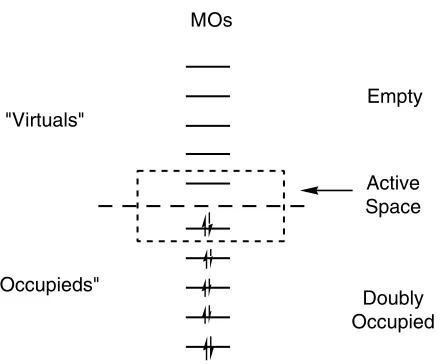
cor-relation and it is normal to use a relatively small number of determinants in the window

or active space (Figure 2-2).† The energy lowering introduced by adding this extra

flexi-bility to the wavefunction so that a better qualitative description is possible is usually

referred to as non-dynamic (or sometimes static) electron correlation. This type of

cor-relation is the result of allowing for near-degeneracy or partial occupancy of the MOs.

The rest of the correlation energy is termed dynamic. An MCSCF wavefunction that

includes the minimal number of determinants to allow for the correct qualitative

descrip-tion recovers only the static correladescrip-tion. In the extreme case, where the active space

includes all MOs, the MCSCF wavefunction is equivalent to full CI and all the dynamic

correlation is also recovered.

2.4.1 Active Space Considerations

The major problem involved in using MCSCF techniques is defining the active

space. This problem has a number of facets. Firstly, a decision needs to be made about

which configurations to include in the MCSCF procedure. The most common MCSCF

technique in use at present is known as the complete-active-space self-consistent-field

(CASSCF) method. Unlike restricted active space (RAS) methods, CASSCF includes in

the SCF procedure all the proper symmetry-adapted configurations resulting from all

†

excitations within the active space. Secondly, based on the problem at hand, one needs

to decide which MOs (both doubly-occupied and empty) are to be included in the active

space.18 Deciding how many orbitals, and which orbitals, to include is not always

straightforward. In order to reduce the time required to compute solutions the active

space is generally chosen to be as small as possible and still give a qualitatively correct

description of the region of a molecule that is being considered. For example, a simple

C–C bond cleavage may be well-described by a [2,2]-CASSCF (which includes two

electrons in two orbitals). However, an inappropriate selection of active space can lead

to an unbalanced description and caution must be used to select the appropriate active

space. One solution is to include all valence electrons (and the corresponding set of

orbitals) in the active space. However, the factorial rise in the number of configurations

generated from the full CI within the active space limits [n,m]-CASSCF to about 12 or 14 electrons/orbitals.

2.4.2 Including Dynamic Correlation

Because MCSCF only recovers a small proportion of the electron correlation, it is

usually necessary to account for the dynamic electron correlation through either

multi-reference configuration interaction (MRCI), which includes all single and double

excita-tions from all reference configuraexcita-tions (i.e. MRCISD), or a perturbative treatment such

Figure 2-2. MCSCF techniques define an active space and determinants resulting from excitations within this space are then included in the SCF procedure.

"Virtuals"

"Occupieds"

MOs

Active Space

Doubly Occupied

as second-order complete active space perturbation theory (CASPT2), which is one of a

number of implementations of many-body perturbation theory as applied to MCSCF.

MRCI calculations are often corrected for a contribution from the quadruples using a

multireference equivalent of the Davidson correction.20 This Davidson-corrected MRCI

is usually written MRCI+Q and has the advantage of size extensivity.

2.5 Basis Sets

As described earlier, molecular orbitals are usually described as a linear

combina-tion of known atomic-centered funccombina-tions. This approach of breaking an unknown

func-tion into a set of known funcfunc-tions is an approximafunc-tion because the basis set is inevitably

incomplete. Increasing the size and/or scope of a basis set until it approaches complete

ness allows for a systematic improvement in the resulting solution (which may however

be incorrect due to other approximations made in the method).

Typically, basis functions are atom-centered although this need not be true. Two

types of atom-centered functions are commonly used. Slater-type orbitals21 (STOs) are

characterized by an exp(–ζr) radial dependence. STOs are the exact solutions to the hydrogen atom problem and therefore provide a good description of atomic

wavefunc-tions, and importantly, they reproduce the correct behavior at the nucleus, where a cusp

should exist. However, gaussian-type orbitals (GTOs), which are characterized by an

exp(–ζr2) radial dependence,22 are by far the most commonly used basis functions. This is a consequence of the cost of calculating the two-electron integrals, which is much less

for GTOs than for STOs. It is expected that more GTOs than STOs will be needed to

properly describe a given wavefunction, both because of the incorrect behavior at the

nucleus and because GTOs are expected to fall-off too rapidly at long distances from the

nucleus. However, the greater efficiency of integral evaluation makes them the basis

functions of choice. In order to improve the properties of an individual basis function,

gaussian-type basis functions are often expressed as a linear combination of primitive

gaussian functions,

(2-21)

where the coefficients (d_µι) and the exponents (ζ) for each of the primitive gaussians (g_i)

φ_µ = d_µi

i

are chosen so as to better represent a true atomic orbital. This type of basis function

(φ_µ), known as a contracted gaussian, is used exclusively in this work and represents a mechanism for improving the form of the basis functions without increasing the

num-ber of basis functions. Keeping the total numnum-ber of basis functions to a minimum is

cru-cial because the time to compute a given system usually rises rapidly (in some cases to

the seventh power) with the number of basis functions.

2.5.1 Split-Valence and Mixed Basis Sets

Selecting a set of basis functions for use in describing the molecular orbitals

(Equation 2-6) generally involves some degree of chemical intuition. To start with, it is

recognized that hydrogen and helium have no core electrons while atoms in the first row

have clearly defined core and valence electrons.

Split-valence basis sets make use of a contraction scheme like that described in

Equation 2-21, and the notion of core and valence electrons, to divide up the primitives

into two components. By reducing the number of basis functions used to describe the

core (by grouping primitives as a single function), this scheme allows more basis

func-tions, and therefore flexibility, to be given to the chemically important valence orbitals

while keeping the total number of basis functions to a minimum. Double-split-valence

or valence-double-zeta (VDZ) basis sets have one basis function per core orbital and

two basis functions per valence orbital, while triple-split-valence or valence-triple-zeta

(VTZ) basis sets have one basis function for each core orbital and three basis functions

per valence orbital. Increasing the number of functions used to describe the valence

electron distribution allows, to some extent, for radial electron correlation. Common

examples of VDZ basis sets are 6-31G23 and cc-pVDZ,24 while 6-311G25 is a

well-known example of a VTZ basis set.

Another method for reducing the total number of basis functions required in a

par-ticular calculation relies on using more basis functions per atom in the chemically

important or difficult-to-describe region of the system. In these so-called mixed basis

sets one might use a 6-311G type basis for atoms in the important region while a 6-31G

basis is used for atoms in less important regions of the molecule. For large systems this

calcula-tion.† Mixed basis sets must be used with caution because they may, if not properly

used, bias a calculation and/or create artefacts.

2.5.2 Polarization and Diffuse Functions

The basic VDZ and VTZ basis sets discussed above (6-31G and 6-311G) do not

allow for polarization of the electron distribution around the nucleus. The electron

dis-tribution can be polarized by interactions with other atoms. In order that the basis set is

flexible enough to accurately describe any charge polarization, so-called polarization

functions are employed. Polarization functions are higher angular momentum functions,

which can combine with other functions in the basis set to allow charge polarization.

These functions also have the effect of allowing for angular electron correlation (i.e.

they allow for non-spherical distributions of the electrons about a nucleus). Basis

func-tions of high angular momentum are very important in correlation treatments.

Diffuse functions are used to properly describe the outlying regions of the

mole-cule. These functions are low angular momentum functions (s and p) with low expo-nents (ζ), i.e. they extend further away from the nucleus. Diffuse functions are gener-ally needed to properly describe species with loosely bound electrons such as anions or

species containing lone pairs.

2.5.3 Pople Basis Sets

The Pople basis sets used in this work have a straightforward nomenclature scheme.

The notation 6-31G means that 6 primitive gaussians are used for each core orbital and

two functions containing three and one primitives are used for each of the valence

orbit-als. In similar fashion 6-311G means that 6 primitive gaussians are used for each core

orbital and three functions containing three, one and one primitives are used for each of

the valence orbitals. Most Pople basis sets start with 6-31G or 6-311G and then extend

them by adding diffuse (+) and/or polarization functions. Details of the nomenclature

†

are best explained through a number of examples:

6-31G(d)23 As for 6-31G described above with the addition of d -func-tions on heavy atoms (i.e. non-hydrogen atoms).

6-311G(d,p)25 The 6-311G basis with addition of d-functions on heavy atoms and p-functions on hydrogen.

6-311+G(2d,p)25,26 As above with the addition of diffuse (s- and p-) functions on heavy atoms and replacing the single set of d-functions with two well-spaced sets of d-functions (one set closer in and the other further out from the nucleus than the single set

in 6-311G(d,p)).

6-311++G(3df,2p)25,26 The 6-311G basis with the addition of diffuse (s- and p-) functions on all atoms, three sets of d-functions and one set of f-functions on heavy atoms, and two sets of p-functions on hydrogen.

These basis sets are relatively small (compared with the correlation-consistent basis

sets described below) and provide considerable flexibility in the choice of basis set size.

They have also been used extensively so their performance in a wide variety of

molecu-lar situations is well-known. For these reasons, we have used these basis sets almost

exclusively.

2.5.4 Correlation-Consistent Basis Sets

The correlation-consistent basis sets24 were designed with the aim of recovering the

correlation energy of the valence electrons. In essence, a step up in quality, for example,

from double-zeta (DZ) to triple-zeta (TZ), involves adding one set of functions to each

of the types already represented plus one set of the next higher orbital angular

momen-tum. The smallest correlation-consistent basis set is referred to as

correlation-consis-tent polarized valence-double-zeta (cc-pVDZ), the next is cc-pVTZ and so on. The

number of contracted functions for first row atoms/hydrogen used in each of these basis

sets is [3s,2p,1d/2s,1p] and [4s,3p,2d,1f/3s,2p,1d]. These basis sets can also be

aug-mented by the addition of diffuse functions (aug-). In this case, one extra set of

func-tions with the same angular momentum as those funcfunc-tions already represented is added

sim-ply AVQZ) basis represents a [6s,5p,4d,3f,2g/5s,4p,3d,2f] basis. Similarly, the

aug-cc-pV5Z (or simply AV5Z) basis represents a [7s,6p,5d,4f,3g,2h/6s,5p,4d,3f,2g] basis. We

have used these basis sets where very large basis sets which approached the basis set

limit were desired.

2.6 Hierarchy of Ab Initio Methods

The relationship between basis set and electron correlation level is summarized in

the Pople diagram3 shown in Figure 2-3.

At the top of Figure 2-3 are various treatments of electron correlation, with

Har-tree–Fock, which includes no electron correlation, at the far left. Successively more

accurate treatments of electron correlation are shown from left to right until FCI, which

takes into account all the electron correlation within the limits of the basis set used, is

reached. Going downwards, the basis sets become successively larger until an infinite

basis set is reached. As we go down the diagonal of the figure, the calculations become

more accurate until the exact solution to the non-relativistic Schrödinger equation is

reached at the bottom right-hand corner. Since the increased accuracy also results in a

Figure 2-3. Pople diagram illustrating the progression of ab initio methods to the exact solution to the time-independent Schrödinger equation (under the Born–Oppen-heimer approximation).

increasing basis set siz

e

more complete electron correlation treatment

HF MP2 MP4 QCISD CCSD(T) MRCI … FCI

6-31G(d)

6-31G(d,p)

6-311G(2d,p)

6-311+G(3df,2p)

aug-cc-pVQZ

aug-cc-pV5Z

infinite basis Exact

Solution

…

greater computational cost (often increasing in dramatic fashion), a balance must be

struck between the desired accuracy and computational cost.

2.7 Density Functional Theory

2.7.1 Kohn–Sham Theory

The density functional theory (DFT) approach to solving the time-independent

electronic Schrödinger equation rests on the proof by Hohenberg and Kohn27 which

showed that the ground-state electronic energy is determined completely by the electron

density (ρ) with a one-to-one correspondence. Unfortunately this proof does not give any clues as to the functional form of this correspondence between energy and density.

By comparing with the equations of wave mechanics (and assuming the Born–

Oppenheimer approximation), it is clear that the functional can be divided into three

parts, a term for kinetic energy (ET[ρ]), one for the Coulombic attraction between nuclei and electrons (EV[ρ]), and one for interactions between electrons, which in turn can be readily divided (with reference to HF theory) into Coulomb (EJ[ρ]) and exchange (EK[ρ]) terms (with correlation implicitly assumed in all terms).

E[ρ] = ET[ρ] + EV[ρ] + EJ[ρ] + EK[ρ] (2-22)

The use of DFT theory in computational quantum chemistry has been facilitated by

a reformulation (by Kohn and Sham28) of the problem of determining the functional

form of the relationship between the energy and density. In this reformulation, Kohn

and Sham introduced an orbital approach by writing the approximate density (ρ(r)) in terms of a set of auxiliary one-electron functions (Equation 2-23).

(2-23)

Further, the kinetic energy is calculated under the assumption of non-interacting

electrons (ETs[ρ]) (a similar approach to that used in HF theory). Equation 2-22 can

ρ( )r ψ_i( )r 2

i=1 N

∑

then be rewritten in the more customary form,

E[ρ] = ETs[ρ] + EV[ρ] + EJ[ρ] + EXC[ρ] (2-24)

where EXC[ρ] is called the exchange–correlation term and by definition includes all con-tributions not accounted for in the first three terms. If the density is expressed as in

Equation 2-23 (and in practice the one-electron functions are rewritten as a linear

com-bination of atomic-centered orbitals), then the functional connection between the density

and the energy for the first three terms of Equation 2-24 is known and the problem is

reduced to finding the functional form for EXC[ρ]. If the exact form for this term could be deduced, then an exact solution to the energy would result. Unfortunately, the exact

form is not known, and what is worse, no means for systematically improving the

func-tional is evident. As a result, all trial funcfunc-tionals must be compared with experimental

results in order to determine their accuracy. It is in this sense that many people do not

consider DFT implementations truly ab initio.

2.7.2 Functionals

The exchange–correlation term (EXC[ρ]) is usually divided into separate exchange (EX[ρ]) and correlation (EC[ρ]) terms, although there is no requirement to proceed in this manner. As a first approximation, it has then been assumed that the density can be

treated locally as a uniform electron gas. This leads to what is called the local density

(LDA) or local spin density (LSDA) approximation. The resulting expressions for EX

and EC are usually referred to as Slater or simply S (because of the similarity of the expression for the exchange term with that proposed by Slater29 in his Xα method) and VWN (after Vosko, Wilks and Nusair30 for their analytic interpolation formula for the

correlation energy of a uniform electron gas), respectively. The LSDA approximation,

although quite simple, performs remarkably well (even though it gives relatively large

errors in the exchange and correlation energies) and is generally considered to do as

well as HF theory.

Improvements over the LSDA approach have come from including dependency on

not only the density but also the gradient of the density in the exchange and correlation

terms. Becke31 has proposed such a correction to the LSDA exchange term. The

pop-ular gradient-corrected functionals for the correlation term is that proposed by Lee, Yang

and Parr32 and is referred to as LYP. This functional is derived from fitting four

parame-ters to data for the helium atom. The resulting gradient-corrected DFT method (B-LYP)

has proven very popular.

Further improvements in the functional result from application of what is called the

adiabatic connection formula (ACF).1 This leads to methods that are termed hybrid

methods because they use a suitable combination of both the exact exchange (of a

sys-tem of non-interacting electrons, i.e. the HF exchange) and a functional exchange term.

The most widely used hybrid method is a three-parameter method33 and is referred to as

B3-LYP,

(2-25)

where ∆B refers to Becke’s gradient correction to the LSDA exchange and the other terms are as detailed above. The three parameters a, b and c are fitted to experimental

data.† This method has been found to give remarkably good results in many situations

(often in good agreement with CCSD(T)) and is the DFT method used exclusively in

this work. However, like all functionals, its performance is only really known for

sys-tems similar to those for which it has been tested thoroughly. As a method for

explor-ing the structure and energies of novel molecular systems (where no experimental data

are available), it is clearly inferior to methods which can be systematically improved, or

at the very least it needs to be tested in such cases against high-level calculations on

model systems.

If confidence can be gained in the performance of a particular functional, DFT can

be a very powerful technique because the computational cost (in terms of compute time)

of even the hybrid methods is considerably less than any other method that allows for

electron correlation.

†

Although there are a number of parameters in both the Becke three-parameter model and the LYP corre-lation functional which are fitted to experimental data, these methods are not usually referred to as semi-empirical. For a discussion of the semi-empirical methods used in this work see Section 2.8 on page 74.

2.8 Semi-empirical Procedures

Unlike molecular mechanics1 (MM) or force-field methods, which treat molecules

as a classical system of particles whose interaction is described by a parametric force

field equation, the so-called semi-empirical methods1 are based on a quantum

mechani-cal description of the molecule. The central assumption taken in the semi-empirimechani-cal

methods34 is the zero differential overlap (ZDO) approximation. This approximation

sets to zero all products of basis functions which depend on the same electron

coordi-nates when located on different atoms.† The result of this is that the overlap matrix

becomes a unit matrix, one-electron integrals involving three centers are set to zero, and

the most numerous two-electron integrals, i.e. all three- and four-center two-electron

integrals, are neglected. The remaining integrals are then replaced with parameters. It

is this parametrization (usually done by comparing with experimental results) which

leads to the name semi-empirical. The various semi-empirical methods differ as to how

many integrals are neglected and how the parametrization is done. To further simplify

the problem, all core electrons are accounted for by reducing the nuclear charge, so only

valence electrons are considered. And finally, a minimum basis set (of s and p

Slater-type functions) is employed.

The most common semi-empirical methods in use at present (and used in this work)

are the methods referred to as Austin model 135 (AM1), and modified neglect of

diatomic overlap, parametric method 336 (PM3).‡

For our purposes, these methods have been used in place of MM methods to find

starting geometries for novel saturated hydrocarbon cage compounds because they were

found to give superior geometries at the central quaternary carbon atom; MM methods

were found to predict pyramidalization and loss of symmetry at the central carbon atom

while AM1 and PM3 gave geometries of correct symmetry (for closed-shell species)

with errors in the bond angles within the accepted limits for these methods (3.5° and

4.0°, respectively).1 Energies from these calculations have not been considered.

†

Note that it is the product of basis functions and not the integral over these products that is set to zero.

‡

2.9 Potential Energy Surfaces

As a consequence of the Born–Oppenheimer approximation, a chemical system is

viewed as a set of nuclei moving on a potential energy surface which is (at each point in

space) a solution to the electronic Schrödinger equation.

2.9.1 Geometry Optimization

For almost all computational problems, it is impractical to calculate the entire

potential energy surface (PES). It is often more convenient to locate points of interest

on the surface, which are usually stationary points. These points are characterized by all

the derivatives with respect to the 3N – 6 (for a non-linear molecule) internal coordi-nates being equal to zero, i.e.

where i = 1, 2, 3 … 3N – 6. (2-26)

There are two types of stationary points that of most interest to chemists. The first

are local minima, corresponding to equilibrium structures. The second are first-order

saddle points, which correspond to transition structures. The two types of stationary

points can be distinguished by examining the eigenvalues of the Hessian, or

force-con-stant matrix, formed by the second derivatives of the energy with respect to the

coordi-nates,

where i, j = 1, 2, 3 … 3N – 6. (2-27)

Equilibrium structures are characterized by having no negative eigenvalues of the

Hes-sian, while first-order saddle points have one negative eigenvalue.

Efficient geometry optimization techniques,1,37,38 for both minima and saddle

points, are implemented into the GAUSSIAN 98 system of programs.39 These allow

sta-tionary points to be located in a relatively straightforward manner for methods that have

readily available analytic first derivatives (HF, B3-LYP, MP2, QCISD, etc.). These

tech-niques employ either an approximate second-derivative matrix (which is updated using

information from the first derivatives and nuclear displacements) or no second-derivative

matrix. As a consequence, true minima must be verified by calculation of the second

∂E

∂r_i =0

∂2

E

derivatives at the optimized geometry, i.e. where the first derivatives are all zero (to

some level of accuracy). The HF, B3-LYP and MP2 methods are among those

imple-mented in GAUSSIAN 98 which allow ready optimization and characterization of the

resulting stationary points.

2.9.2 Normal Mode Analysis

Vibrational frequencies can be calculated by diagonalization of the force constant

matrix (Equation 2-27), calculated by analytic or numerical second derivatives. The

resulting values are known as normal-mode frequencies. An equilibrium structure is

characterized by all frequencies being real while a first-order saddle point or transition

structure has one imaginary frequency.

The harmonic approximation used in the calculation of normal mode frequencies

leads to systematic errors; the calculated frequencies are usually larger than

experimen-tally determined frequencies because of anharmonic contributions to the observed

fre-quencies and inadequacies in the calculations.40,41 Consequently, the calculated

frequen-cies are often scaled to take into account the effects of the neglect of anharmonicity,

incomplete electron correlation and basis set deficiencies. Scaling factors for many

methods and basis sets (which have been determined by comparison with a wide range

of experimental data) are available.40

2.9.3 Zero-Point Energies

Because nuclei are not a set of classical particles but form a quantum system, the

true energies of a system of nuclei at any given point on the PES require a correction

which takes into account the zero-point vibrational energy associated with that

geome-try. When determining or comparing results from MO calculations with experiment (for

example heats of formation), it is necessary to add to the calculated energies a correction

for this zero-point energy. The zero-point vibrational energy (ZPVE) is given by

(2-28)

where ν_i are the scaled vibrational frequencies in appropriate units. It should be noted ZPVE 1

2

---h ν_i

i

∑

that the optimum scaling factors for frequencies and zero-point energies often differ.40

2.10 Molecular Properties

2.10.1 Symmetry

Although symmetry is not strictly a molecular property it is indeed a geometric

property of many molecular systems. We have found in this work that the use of

molec-ular symmetry wherever possible has been of tremendous advantage. Because many

computational algorithms are able to make use of molecular symmetry (for example this

leads to block diagonalization of the overlap matrix), this can significantly reduce the

time needed for calculations on a system. In principle, compute time is reduced by a

factor of two for each order of symmetry (so D₂ symmetry reduces the computational cost by a factor of eight). In practice, sparse matrix techniques and other algorithmic

improvements give better savings in compute time for molecules with little or no

sym-metry so the gain from making use of symsym-metry is somewhat less but it can still be quite

considerable for high symmetry structures like dimethanospiro[2.2]octaplane (2-1).†

2.10.2 Strain Energies

The concept of strain is inexact. However, it is extremely useful conceptually.42 It

generally refers to the increase in energy of a molecule that results from structural

devia-tions from the ‘norm’. The effects of strain are generally discussed in terms of bond

angle and bond length distortions, torsional effects, non-bonded interactions and so on.

All of these effects refer to structural variation that can be seen to raise the energy of a

molecule. The main problem with a rigorous definition of strain is that a reference point

must be chosen. The usual definition of strain in hydrocarbon systems takes the

mole-cules methane, ethane, propane, isobutane and neopentane to be strain-free. Essentially

this defines the reference energy for methane and primary through to quaternary carbon

centers. This definition can be extended to include further compounds (for example

ole-†

fins) by defining further reference compounds (in the case of simple olefins one would

need to include propene and 2-methylpropene).

Such a definition of strain for saturated hydrocarbons, in which the strain energy is

given relative to the simple hydrocarbons (listed above), leads to a direct method for the

calculation of strain energies (SE).43 This involves writing a homodesmic reaction in which the target molecule is broken down into the unstrained hydrocarbons. For

exam-ple,

spiropentane + 6 ethane neopentane + 4 propane (2-29)

The associated total strain energy (SE) of spiropentane is the negative of the enthalpy (–∆Hhomod) of the resulting reaction (Equation 2-29). Such a reaction is termed homo-desmic because the number of primary, secondary, tertiary and quaternary carbon atoms

and the number of bonds between atoms of the same hybridization on each side of the

reaction are balanced. The aim in such a scheme is to maximize the cancellation of

errors in the calculation of the enthalpy change. In order to obtain a true reaction

enthalpy, the calculated energies are corrected for the ZPVE (as described above). The

resulting entropies at 0 K are corrected to 298 K using the formula,

(2-30)

where, (2-31)

(RT for linear molecules) (2-32)

(2-33)

assuming ideal gas behavior (N is Avogadro’s number and h is Planck’s constant). As with calculation of the ZPVE, scaled, calculated frequencies are used to calculate

∆H_vib(T), but a scale factor appropriate for reproducing temperature corrections is used.

Strain energies calculated in this way represent the total strain energy (SE) of a molecule. In this work we have found it useful in some cases to calculate strain energies

∆H T( ) = H_trans( )T +H_rot( ) ∆T + H_vib( )T +RT

H_trans( )T 3

2 ---RT

=

H_rot( )T 3

2 ---RT

=

∆H_vib( )T Nh νi ehνi⁄kT –1

( )

---i

∑

that are more localized to a certain region of a molecule by deducting the strain energy

inherent in the remainder of the molecule. Such schemes are explained in detail where

used.

2.10.3 Heats of Formation

Heats of formation allow for the relative energies of molecules to be compared in

an absolute sense. They also allow for comparison between calculation and

experi-ment. The method used for the calculation of heats of formation in this work is based

on that of Schulman and Disch.43 The heat of formation is determined from the

calcu-lated enthalpy of the same homodesmic reactions used to calculate the total strain

energy (e.g. Equation 2-29) together with the experimental heats of formation of the

unstrained hydrocarbons used to balance the homodesmic reactions. Again using the

example of spiropentane, the expression for the calculated heat of formation (at 298 K)

can be written,

∆H_fcalc(spiro) = SEcalc + ∆H_fexp(neo) + 4∆H_fexp(pro) – 6∆H_fexp(eth) (2-34)

where SEcalc, the total strain energy, is calculated as described above, and the labels neo, pro and eth refer to neopentane, propane and ethane, respectively.

2.10.4 Proton Affinities

Knowledge of the energetics of the reaction in which a molecule attracts a proton

has many applications in chemistry. Very strong bases can be used in reactions as

pro-ton sinks or to remove a propro-ton from a molecule to enable further reactivity. One way of

expressing this property is as a gas-phase proton affinity (PA). Gas-phase proton affini-ties (PA) can be determined as the negative of the enthalpy of the protonation reaction,44

B_(g) + H+_(g) BH+_(g) (2-35)

2.10.5 Ionization Energies

The first adiabatic ionization energy (IE) indicates the ease or difficulty of remov-ing a sremov-ingle electron from a molecule. Knowledge of the strength with which electrons

are bound to a molecule is important in designing systems where electron transfer is

facilitated. Adiabatic ionization energies are calculated as the negative of the enthalpy

change in the following reaction,

B_(g) B+_(g) (2-36)

where B is the molecule in question. If B is a ground-state closed-shell system then B+

will be an open-shell doublet state and will need to be treated with a method suitable for

dealing with open-shell systems. In our calculations of ionization energies we have used

the UMP2 method. Correction of the energy difference for ZPVE and to 298 K allows

for comparison against experimentally determined IEs.

2.11 Computational Resources

2.11.1 Software

The main software package used for the ab initio calculations in this work was GAUSSIAN 98.39 The SPARTAN system of programs45 was used extensively for

visualiza-tion purposes and for initial structure design studies. This initial design stage usually

involved making use of SPARTAN’s semi-empirical algorithms (in almost all cases AM1

was preferred). Calculations employing higher-level correlated techniques (CCSD(T),

MRCI, etc.) were carried out using the MOLPRO system of programs.46 One of the two

numerical MP2 second derivatives reported here was calculated using GAMESS.47

2.11.2 Hardware

The majority of calculations in this work were performed using the Fujitsu

VP-2200, VPP-300, SUN E4500 and SGI PowerChallenge of the Australian National

Uni-versity Supercomputing Facility (ANUSF) and various IBM RS/6000 workstations

situ-ated at the Research School of Chemistry, Australian National University. A large

pro-portion of the B3-LYP calculations were run on the IBM SP systems at the Maui High

2.11.3 Resource Usage

In the discussion so far, we have alluded on occasion to the cost in terms of

com-puter time required to generate solutions for the various methods. Generating solutions

can become computationally very expensive either for very high-level correlated

meth-ods (like CCSDT), or when the number of basis functions employed becomes large,

either through use of a large basis set or when large systems (with many atoms) are

being examined. For large systems (like, for example, the spiroalkaplanes (2-2)) even methods which we have indicated as being relatively cheap, like MP2, can become

com-putationally expensive. As a result, whether or not a method can be used, or a system

can be studied, often depends on the efficient implementation of a method on a

particu-lar computer platform. The algorithms used, and the implementation of those

algo-rithms, on each computer platform, can have a major effect on what problems can be

attempted with any given hardware. To the pure theoretician the matter of

implementa-tion may seem a trivial matter of writing computer code. In practise this is anything but

simple. The task of implementation is complicated in part because their may not be a

unique way of defining a method (e.g. perturbation methods applied to MCSCF).

Fur-ther complications arise from the need or desire to tune or optimize the code to get

max-imum performance from the available hardware. Thus the rapid pace of hardware

devel-opment acts as both a boon and a bane; the increased performance of new generations of

computer technology allow much larger problems to be examined but the introduction of

new hardware designs makes carefully-tuned codes rapidly obsolete.

A further problem that becomes obvious as larger systems are considered is that

Moore’s Law (see Section 2.1 on page 51) only predicts a doubling of processing speed

for each year or so, while the computational cost of most methods increases with a much

higher power. For example, the compute time to solve MP2 gradients formally

increases with the order ON4, where O is the number of occupied orbitals and N is the

number of basis functions, while a CCSD(T) energy calculation scales as O3V4, where V

represents the number of virtual orbitals.48 This means that the size of systems being

examined with these correlated techniques can only increase gradually from

year-to-year.

The introduction of linear scaling techniques for HF and DFT methods, such as

tyranny of exponential scaling in compute times. However, these methods all appear to

introduce considerable up-front cost and the break-even point is usually somewhere

beyond 50 atoms.† Further, DFT is the only method to date which includes electron

cor-relation and which can be treated with these techniques. This suggests a bright future

for DFT, especially if a means of systematically improving functionals can be derived.

Attempts to study relatively large systems (in this work molecules as large as 25

carbon atoms and 24 hydrogens have been considered in detail using correlated ab ini-tio techniques) involve considerable effort in choosing the most efficient algorithms and maximizing usage of the available compute time. As an example, even the modest

increase in molecular size from spiro[2.2]octaplane (C₂₁H₂₄) (2-2) to dimethano-spiro[2.2]binonaplane (C₂₅H₂₄) (2-3), an increase of exactly four carbon atoms, leads to an increase in the compute time for an MP2/6-31G(d) gradient calculation (see

Section 2.12 on page 84) in C₁ symmetry using GAUSSIAN 9839 (which we find to be the most efficient package for single-processor MP2 calculations) of about 100%, i.e. a

dou-bling of the compute time. This equates to an extra 5 days of compute time on an RS/

6000 processor or 15 hours on a single VPP-300 processor.

The full ramifications of such large compute times can be seen when one considers

the time required to compute the MP2 second derivatives for

dimethanospiro[2.2]octa-plane (2-1) and dimethanospiro[2.2]binonaplane (2-3). These calculations were done numerically (using a double differencing method) rather than analytically for two

rea-sons. Firstly, the analytic second derivatives can not be restarted during the calculation

†

This is quite variable and actually depends on the three-dimensional shape of a system. The initial set-up cost for such linear-scaling calculations is least for linear systems (like all-E-dodecahexaene), greater for planar systems (for example a graphite fragment) and greatest for globular systems (like the alkaplanes or proteins).

2-2