International Journal of Innovative Technology and Exploring Engineering (IJITEE) ISSN: 2278-3075,Volume-8, Issue-10, August 2019
Abstract: Tracking the location of target nodes/objects plays a vital role in disaster management and emergency rescue operations. The wireless sensor network is an easiest and cheapest solution to track the target nodes/objects in emergency applications. Use of GPS installed devices in wireless sensor networks is one of the solutions to track the target node’s location. Installing GPS device on every target node is very expensive and the GPS device drains the battery power, and increases the size of sensor nodes. Localization is an alternative solution to track the target node’s location. Many localization algorithms are available to track/estimate the target node’s location coordinates, but the accuracy of the estimated target nodes is poor. A new localization technique is proposed in this work to improve the accuracy of the estimated location of the target nodes. The proposed technique uses two anchor nodes, and parameters like linear vector segments, received signal strength, and angle of arrival measures in the location estimation process. This work has been simulated in MATLAB. The proposed algorithm outperforms the existing localization techniques.
Index Terms: Angle of Arrival, GPS, Localization, Received Signal Strength.
I. INTRODUCTION
Interconnected wireless sensor nodes form a wireless sensor network. Each and every sensor node in the sensor network may consist of various hardware modules such as RF transceivers, micro controller, memory and power unit [1]. In general, every sensor node in the network collects data and transfer the data to the sink node or central node for further activities [2]. Every node in wireless sensor networks has computing capability and also processing capability to process the data itself. Many applications use wireless sensor network services in order to monitor, control, and analyze their activities [3]. Many applications (automation) in the real world need wireless sensor networks for controlling many activities [4]. The location information of the sensor nodes can be used in many applications [5]. The data collected by the sensor network can be less useful if it does not have location information [6]. Placing the GPS device on each and every sensor node in the sensor network is a very time-consuming process, and very costly. Localization is an alternate solution in WSN to get the target node’s location information [7]. There are two localization techniques available in WSN; namely anchor based and anchor free
Revised Manuscript Received on August 05, 2019
Mamidi Kiran Kumar, Department of Computer Science and
Engineering, JNTUH College of Engineering Hyderabad, Hyderabad, India.
V. Kamakshi Prasad, Department of Computer Science and
Engineering, JNTUH College of Engineering Hyderabad, Hyderabad, India.
localization techniques. An anchor is a node in the sensor network, and which knew its location information already. Based on the computational technique, localization techniques are classified into two types; namely Centralized and Decentralized. The Fig 1, illustrates the classification of localization techniques. In the centralized localization techniques, a network has a high computational sink-node or base station, and all other sensor nodes transfer their data to the sink-node. Whereas in decentralized localization technique, each and every sensor node in the sensor network can also process data along with collecting data [8].
Figure-1: Localization Algorithms-Classification Decentralized localization techniques are divided into two classes; namely Range based localization and Range free localization techniques. The range based localization techniques use RSS (Received Signal Strength), AOA (Angle of Arrival), TOA (Time of Arrival) and TDOA (Time difference of Arrival) distance measures in localization. The range-free localization techniques use Proximity, Known locations, and Hop count distance measures in localization [9]. Centroid and DV Hop (Distance Vector Hop), and APIT (Approximation Point in Triangle) are the range free localization techniques [10]. Trilateration, Multilateration, and Triangulation are range-based localization techniques [11]. The accuracy of the estimated value of the target node is very poor in the range free localization techniques, but the accuracy is very high in range based techniques [12] [13]. A
novel range based localization algorithm, namely Triangular
Areas Segmentation-based Localization Technique (TASLT) is proposed to achieve better accuracy for WSN, and it uses a lookup table and static
DALT: Double Anchor-Based Localization
Technique for Wireless Sensor Networks using
RSS and AoA Measures
vectors in location estimation process [14]. The challenges in the TASLT method like a poor accuracy and the use of a lookup table, can be addressed in this paper. We proposed a range-based localization technique which does not use lookup table and improves the localization accuracy by using dynamic linear vector segments.The proposed localization technique uses coordinates of the two anchor nodes, AoA based linear vector segments, and the distances between the target node and the anchor nodes for determining the target node location. The main idea behind the proposed method is to improve the accuracy of the estimated target node location coordinates in a simple manner. The performance of the proposed method can be measured using the metrics such as total error, average error, and accuracy. The proposed method has been simulated in MATLAB-14a. It performs much better than traditional localization methods. The main contributions of this paper are:
1) A localization algorithm based on two anchor nodes. 2) Collection of RSSI and AOA measures at every
anchor node for developing and computing the required things for the next phases.
3) Creation of dynamic vectors by using the proposed mathematical functions.
4) Use of vector’s segment information at every anchor node to determine the target node values.
5) Enhancement of the final results done by averaging the partial results of the target node with respect to every anchor node.
The remaining sections are organized as follows. The survey related to the work is presented in the section-II, The proposed localization method is described in the Section-III, the experimentation and results are presented in the Section-IV and finally, the conclusion and future work are discussed in the Section-V.
II. LITERATURE
In order to get the best accuracy in localization applications, a lot of research has been carried out in the localization of WSN. In this section, The distance measures such as RSSI, AoA and localization methods such as trilateration, multilateration, triangulation and single anchor based localization techniques like TASLT are described. A. Distance Measures
1) RSS (Received Signal Strength) is used to calculate the distance between sender/transmitter and receiver. If the distance between the sender (source) and the receiver (destination) is increased, the power of RSS will be decreased. There is no special hardware required to perform the RSS based distance estimation in the WSN, because of antenna availability on every node. The RSS is sensitive to environmental factors, but does not consume more battery of sensor nodes. The accuracy of the RSS based distance is moderate. The RSS based distance between the target nodes and the anchor node can be estimated by using the following “(1)”[15].
0 10 log ( ) 1010 log ( ) 27.5610 d
P P n f n d (1)
Where: ‘P0‘ the signal power (dBm) at zero distance between sender & receiver, ‘Pd’ is the signal power (dBm) at the distance ‘d’, and ’ f’ is the signal frequency in GHZ (2-GHZ) and ‘d’ is the distance (meters) between the receiver
and the sender, ‘n’ is the path-loss constant (for free space n=2) and the fading effect in ‘IEEE 802.15.4 network’s value is 27.56.
2) AoA (Angle of Arrival) can be used to calculate the angular direction of the receiving signal at anchor node. AoA is determined at every anchor node by using special hardware (array of antennas or electromagnetic compass) [16]. The directional antennas are to be installed on anchor nodes, and the orientation of the antennas is to be adjusted in the network appropriately. The accuracy of AoA is higher than the RSS [17].
B. RANGE BASED LOCALIZATION TECHNIQUES
1) Triangulation is one of the localization techniques and is a simple trigonometric approach. Three anchor nodes used in the triangulation and are equipped with special hardware on these anchor nodes to estimate the direction of the received signals. Array of antennas or electromagnetic compass can be used as special hardware on the anchor nodes. Angle of Arrival (AoA) of a received signal can be used to estimate the distance between the target node and the anchor (reference) nodes. The target node location can be estimated using three distance measures and locations of the anchor nodes. Let T1 (x, y) is the target node’s coordinates and A1, A2 and A3 are the anchor nodes. Let αy1, αy2, αx1, and αx2 are the direction of the received signals at the given the anchor nodes. The following “(2),” can be used to calculate the target node coordinates T1 (x, y) [19]. The accuracy of the triangulation method is better good, but this method needs a special hardware on every anchor node to get the good results.
Figure-2: Localization using triangulation
1 2 1 21 2 1 2
sin( )sin( ) sin( )sin( )
, ,
sin( ) sin( )
ry y y rx x x
y y x x
d d
x y
(2)
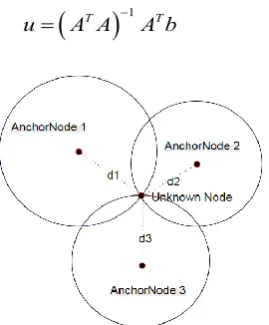
2) Trilateration is a simple geometry-based approach to determine the coordinates of the target nodes by using three non collinear anchor nodes, as well as target node’s distance from the anchor nodes. The target node can be existed at the intersection point of the three circles drawn from the anchor nodes, where the radius of the circles is the distance between the target node and the anchor nodes. Trilateration is simple, and easy to implement, and which doesn’t need a special hardware on every sensor
International Journal of Innovative Technology and Exploring Engineering (IJITEE) ISSN: 2278-3075,Volume-8, Issue-10, August 2019
distances from the target node to anchor node-1, anchor node-2, and anchor node-3 are
d
1,d
2, andd
3 respectively. Todetermine the location of the target node, the estimated distances and locations of three anchors can be used. All these three linear equations can be represented as a least square equation form to get the target node (x, y) coordinates,
this process is called as trilateration.
LetA x y11, 1, ( , ), ( , )A x y2 2 2 A x y3 3 3 as anchor nodes and,d d d1, ,2 3 as the distance from anchor nodes to the target node u x y( , )u u respectively. By using the LSM (least square method) [21], the target node ‘u’ can be estimated by using the following “(3)”.
T
1 T [image:3.595.107.242.235.398.2]u A A A b (3)
Figure-3: Localization Using Trilateration Method
3) Multilateration is same as the trilateration technique, but the number of anchor nodes is greater than three anchor nodes [22]. The location of the target node can be determined using more than three linear equations. The accuracy of the estimated node values in multilateration is more than the trialtaration. In the Fig 3, there is a target node that can be existed at the intersection point of three circles drawn from the anchor nodes where the radius of the circles is the distances between the target node and the anchor nodes. The distance from the target node to the anchor node A1 is d1, from the anchor A2 is d2, and from the anchor A3 is d3 and so on.
4) Single Anchor based localization: A novel range based localization method, namely Triangular Area Segmentation based Localization Technique (TASLT) is proposed to achieve better accuracy in WSN [14]. RSS and AoA distance measures are used to implement the TASLT localization technique. This method uses static vector segment’s information and a lookup table in the location estimation process. In this method, The estimated target node values are not be the user desired level, and the estimated node values have too much error if the target node is very far from the anchor node location.To use static vector segment’s information, an anchor must be searched in the lookup table. This technique has to spend some time on searching of vector segment data that is to be selected for the location estimation process. Every anchor node is to maintain extra memory to hold lookup table data. To improve the accuracy of the
estimated node values as well as to avoid usage of the lookup table concept, a new localization technique is proposed which uses dynamic vectors and two anchor nodes in the localization process.
[image:3.595.309.553.305.428.2]III. PROPOSEDLOCALIZATIONMETHOD The proposed localization method is a simple geometry based approach and is implemented using two anchor nodes to improve the accuracy of the target node values, whereas TASLT used only a single anchor node to estimate the target node values. In this method, dynamic linear vectors can be used in the location estimation process at every anchor node. The accuracy of the proposed work is improved than the TASLT localization method. The proposed method has three phases which are 1) data collection, 2) Creation of dynamic vectors, and 3) Target node location estimation. The proposed localization technique has been implemented by considering the following architecture given in the Fig 4.
Figure 4: Block Diagram Of The Proposed Localization Technique: A Three-Phase Approach
A. Network Architecture
[image:3.595.301.556.515.698.2]The proposed research work uses the following parameters in the network setup.
Table 1: Parameters for the proposed research work network setup Sl
No Simulation Parameters Value/ Status 1 Network Area ½*70*70m=2450 square meters 2 Anchor Nodes Deployment Manual and strategic (Right angle
Triangle) 3 Environment Outdoor /Indoor 4 Distance measures RSSI and AoA 5 No.of Anchor Nodes 2
6 Communication range
between Anchors Max 100 meters 7 The antenna used on Anchors Directional 8 Antennas used on Targets Omni Directional 9 Special H/W on Antenna
(Anchors)
Electromagnetic Compass/ Array of Antennas
10 Channel (on Anchors) Dual (Anchor to anchor and anchor to Target)
11 Channel (on Target) Single (Target to Anchor) 12 No. of Targets 7 (Seven in the triangular area) 13 Communication Protocol Zigbee (IEEE 802.15.4)
This research work used suitable distances to maximize the localization area and to get good localization accuracy. The anchor node ‘A’ and the anchor node ‘B’ is deployed as shown in the above Fig 5.
meters (uses zig-bee communication protocols) and the distance between the anchor node ‘A’, and the anchor node ‘B’ is 98.99 meters. The anchor nodes use directional antennas (Coverage angle is 450) and these anchor nodes are to be faced towards each other. The coverage area of the anchor nodes is ½*70*70m (2450 square meters). Target nodes are to be equipped with omnidirectional antennas and in the coverage area of the double anchors, the target nodes move. In the given setup, ‘AC’ is the horizontal reference line, ‘BC’ is the vertical reference line, and the reference lines are ‘70’ meters long. The nature of the anchor nodes ‘A’ and ‘B’ are static, and they have their position information in advance (manually configured or use of a GPS device). All the target nodes are mobile in nature and they don’t know their location information. As shown in the Fig 5, the target node ‘T’ is in the two anchor's triangular cover area. Here, the target nodes are also shown in black and gray color in the Fig 5. If the target node moves in the two anchor's coverage area, two anchor nodes connect to the target node automatically.
Figure-5: Localization using the Proposed Method B. A THREE PHASE APPROACH
The proposed method has three phases; namely 1) Data collection 2) Creation of dynamic vectors and 3) Target node estimation.
1) First Phase (Data Collection): After completion of the network setup for a triangular area, RSS and AoA data can be collected. The Received Signal Strength (RSS) of the target node can be collected at every anchor node separately. The collected received signal strength can be converted into distances by using the RSSI path-loss model given in “(1)”. The distance between the target node (Unknown) and the anchor node ‘A’ is ‘AT’ (i.e. distance ‘da’) as well as the
distance is ‘BT’ (i.e., distance ‘db’) with respect to the anchor
node ‘B’. Once the coordinates of anchor node ‘A’, the distance between the anchor node ‘A’ and the target node ‘T’ (‘AT’) are known, the distance da can be calculated easily by
using the Euclidian distance formula. The Angle of Arrival (AoA) of the target node’s signal can be calculated at every anchor node. In real-time applications, an electromagnetic compass or an array of antennas can be used on anchor nodes
to determine the angle of arrival of a signal. In this simulation work, Angle between two vectors formula is used to get the AoA. A line from the anchor ‘A’ to the target ‘T’ is drawn and it makes an angle ‘Q1’ with the vector AC (i.e, Horizontal reference line), as well as a line from the anchor ‘B’ to the target ‘T’, which makes an angle ‘Q2’ with the vector ‘BC’(Vertical reference line). The angles Q1 and Q2 can be used to create the dynamic vectors V11, V12, V21, and
V22.
2) Second Phase (Create Dynamic Vectors):
Usually, the angular error, i.e., ‘1’ degree (δ=1) added and subtracted with the incident angle (‘Qi’) to get two more new
angles. Creation of two dynamic vectors can be drawn based on the obtained two angles. Drawing of dynamic vectors and identifying vector segment points on the vertical reference line can be performed by using the rules given in “(6),” and “(8)”. In the given Fig 5, angular error (i.e., δ= 1 degree) is subtracted from the Q1 to get the new angle ‘a11’ and added to
the Q1 to get the new angle a12. Similarly, the angles a21 and
a22 can be formed by using Q2. The anchor ‘A’ point of view,
the vector segment points on vertical reference line ‘p’ such as S1= (b, p1) for vector V1,1 and S2= (b, p2) for vector V1,2 by
using the anchor node ‘A’ coordinates (X1, Y1) and [b, pj =
b*tan (a1j)].
0 0
1
1 1
1 ' ' 1 1,2, 1 , [0,45 ]
1 1
( )
tan( ) , ,
( )
j j
j foranchor A j j Q
j a Q p
a where a
a Q
b
(5)
1 11 1 1,1
' '
2 12 2 1,2
* tan( )
int'
* tan( )
foranchor A
p b a p V
Vectorpo s
p b a p V
(6)
The anchor ‘B’ point of view, the vector segment points on horizontal reference line (‘b’) such as M1= (p, b1) for vector V21 and M2= (p, b2) for vector V22 by using the anchor node
‘B’ coordinates (X2, Y2) and [p, bj=p*tan (a2j)].
0 0 1
2 2
2 ' ' 2 1,2, 1 , [0,45 ]
2 2
( )
tan( ) , ,
( )
j j
j foranchor B j j Q
j
a Q
b
a where a
a Q
p
(7)
1 21 2 21
' '
2 22 2 21
* tan( ) int'
* tan( ) foranchor B
b p a b V
Vectorpo s
b p a b V
(8)
3) Third Phase (Target Node Estimation): After collection of the target node’s data, and creation of dynamic vectors for every anchor node, this phase is to be performed for the target node estimation. Vector segments points, the distance between the anchor node and the target node can be used to form three linear equations with respect to every anchor node. The target node location coordinates can be calculated by solving the linear equations together. The steps involved in this phase are explained in the following algorithm.
The following algorithm explains the step by step processes involved in the proposed method.
Algorithm (da, db, α, R, Q1, Q2,a11, a12, a21, a22, Xa_estv, Ya_estv, Xc_estv, Yc_estv, Xest, Yest)
{
Input: ‘N’=the number of sensor nodes, R= the transmission range of every node (R=100 meters)
Output: (Xest, Yest ) Target node estimated position
International Journal of Innovative Technology and Exploring Engineering (IJITEE) ISSN: 2278-3075,Volume-8, Issue-10, August 2019
1. Initialize ‘k=2’, ‘k’ is numbers of anchor nodes in the sensor field and ‘N’ is the number of target nodes
//Network setup
2. Place the anchor nodes at the corners of the right angle triangle, and the two anchors should be the extremes of the hypotenuse 3. for each Anchor node k do
//Angle and Distance Measurements
4. If target nodes are within the transmission range of Anchor node_A then
5. for Ancho_ node_A do
6. Retrieve distance (da)between Anchor node_A and the target node using RSSI.
7. Retrieve incident angle (Q1 )of the target node at Anchor node_A using the electromagnetic compass/ array of antennas.
// Creation of Dynamic Vector Segments,Q1,& Q2) are
incident angles of target from Anchor A & B respectively 8. Consider incident angle ‘Q1’.
a11 (Q1 ) and a12 (Q1 )where 1 (0error in AoA_ _ ) 9. Use a11, a12 and trigonometry principles to draw the vector segments from every anchor and identify vector segment points on the horizontal and vertical reference lines. //Position Estimation
10. Estimate the Target node ‘T’ partial position using vectors Vi,j and Vi,j+1 with respect every anchor node.
11. Find Xa_estv and Ya_estv by averaging the partial positions of target node ‘T’values.
12. Repeat the step 4 to 11 w.r. t Anchor_node_B then, we get (Xb_estv, Yb_estv) values.
//Estimation of the final coordinates of the target node 13. End for
14. Find the target node coordinate values (final values) i.e., (Xestv, Yestv) by averaging the (Xa_estv, Ya_estv) and
(Xc_estv, Yc_estv). }
Mathematical computations used in the proposed method are given in the algorithm as step-2 to 5 with respect to the vector V11 and are explained in the following.
1. Let the anchor node ‘A’ coordinates are (X1, Y1), the
target node ‘T’ coordinates are (Xt, Yt), and the
distance between the target node and the anchor node is ‘da’.
2 2 2
(
)
(
)
a i t i t
d
x
x
y
y
(9) 2. Here, the anchor and the target nodes can communicate with each other using zig-bee radio signal. The distance between these two nodes is ‘da’and it can be calculated using the RSSI path loss method.
0 P 10* *log10( ) 27.56
10
10
d
P n f
a
d
(10)Here: ‘Pd’= The received signal power (dBm) at distance ‘da’,’ P0’= the received signal power (dBm) at ‘zero’ distance from the antenna, ’ f’= the signal frequency in MHZ (2400MHZ) and ’da’= the distance (meters) from the anchor to the target node, ‘n'= the path loss exponent (for free space n=2) and 27.56 is the fading effect in IEEE 802.15.4 networks.
3. The slope of a vector segment can be calculated using the following formula given in “(11)”: Vector point (X1, Y1) and vector point [b, Pi= (b*tan (α)].
1 1
1 * tan( )
b y m b x
(11)
Here’ b’ is the length of the horizontal reference vector AC, and ‘α’ is the angle between the vector V11 and the reference vector ‘AC’.
4. Selected Linear Vector segment V11 (i.e, AS1) is
given in “(12)”.
1 1 1
(
y y
)
m x x
(
)
(12) 5. Consider the equations from “(9),” to “(15)”, to get the target node values (Xa_est, Ya_est) with respect tov
11 vector. The equations “(14),” and “(15)”represent the coordinates of the target node.
T
a v_ 11( , ) (
x y
x
a est_ 1,
y
a est_ 1)
(13)2 _ 2 1 1 1 a a est d x x m
(14)
2 1
_ 1 2 1 1
1 1
* tan( )
1 a a est
d
b y
y x x y
b x m
(15)
At anchor node ‘A’, The vectors V11 and V12 are used to get
the partial target node values as shown in “(6)”. The target node Ta (x, y) values can be estimated by averaging the
partial target node values as shown in “(17)”.
_ _ 11,
_ _ 12
( , )
arg ( , )
( , )
a esti a esti a
at anchorA a esti a esti
x y v
T et T x y avg
x y v
(16)
2 2
1, 1 1, 1
( ) ( ) ( , ) , 2 2 j j ij ij a
i j i j
v x v y
T x y
(17)At anchor node ‘B’, The vectors V21 and V22 are used to get
the partial target node values as shown in “(8)”. The target node Tb (x, y) values can be estimated by averaging the
partial target node values as shown in “(19)”.
_ _ 21,
_ _ 22
( , )
arg ( , )
( , )
b esti b esti b
at anchorB b esti b esti
x y v
T et T x y avg
x y v
(18)
2 2
2, 1 1, 1
( ) ( ) ( , ) , 2 2 j j ij ij b
i j i j
v x v y
T x y
(19)The final coordinate values for the target node Tf (x, y) can be computed by averaging the partial target node values: Ta
(x, y) and Tb (x, y) at anchor node ‘A’. The procedure used to
calculate the Ta (x, y) and Tb (x, y) are given in “(17),” and
“(19)”. The final coordinates of the target node Tf (x, y)
values are computed using “(20)”.
( ) ( ) ( ) ( )
( , ) ,
2 2
a b a b
f
T x T x T y T y
T x y
(20)
IV. EXPERIMENTSANDRESULTS
The proposed research work is simulated in MATLAB 15a. The parameters which have been taken into account to implement the work is given in the Table 1. The final target node coordinates values are estimated by using “(20)”. Only seven target nodes are considered to show the performance of the proposed work. All the seven nodes come under the coverage area of two anchor
the anchor nodes (A and B), the distance between the target node and anchor nodes at very anchor (
d
a andd
b),newly formed angles. Here, T1 to T7 are the target nodes and T1’ to T7’ are estimated coordinate values of the target nodes. T-T’ is the estimated error between the actual node and the target node. ‘Q’ is the incident angle and
a
11,a
12,a
21,and
a
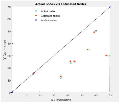
22 are newly formed angles. [image:6.595.64.271.504.682.2]The Table 3 shows the comparison of the estimated target node values by using various methods. The last column of the table 3 consists the estimated values of the proposed method. The following Fig 6 shows the scatter plot for the actual nodes and the estimated nodes. The Fig 6 uses the Table 2 information to draw the plot.
Figure-6: Scatter plot for Actual nodes v/s Estimated nodes
The performance of the proposed technique is determined using the performance measures such as total error, average error, and accuracy. Here (Xe, Ye) represents the coordinates of estimated node values, (Xi, Yi) indicate the coordinates of actual nodes, ‘Nt’ (Nt=7) indicate the number of target nodes and ‘R’ represents the range of anchor nodes(R=100 meters).
2
2 1t N
e i e i
i
TotalError
x x
y y
(21)t
TotalError AverageError
N
(22)
AverageError
Accuracy
R
(23)
The following graphs are drawn using the values of the Table 3. The Fig 7 shows that the accuracy of all the existing methods along with the proposed method. In the Fig 7, the X-axis indicates various methods and the Y-axis indicates the accuracy in percentage. Fig 8 shows that the number of anchor nodes used in various localization methods, and The X-axis indicates various methods and the Y-axis indicates the number of anchor nodes. Two anchor nodes can be used by the proposed technique in localization to improve the accuracy than the single anchor node-based method. This method uses two anchor nodes in localization, whereas the trilateration, multilateration, and triangulation uses three or more anchor nodes for the localization. The accuracy of the proposed method is 98.88% and is higher than all other existing methods.
Table-2: Proposed method based- Estimated Location Coordinates
Sl No
Target Node Coordinates
(T)
Anchor Node Coordinates
A (0,0) B (70,70)
Distance Between anchor and
target
(based on RSS )
da and db
Incident angle of Target node
(Q)
Angle for first Vector (a11=Q1-δ)
(a21=Q2-δ)
δ=1
Angle for second vector (a12=Q1+δ)
(a22=Q2+δ)
δ=1
Estimated Location
T’(Xest, Yest)
Error (T-T’)
1 T1 (45,25)
A 48.96 29.05 28.05 30.05 T1’
(44.51,25.48) 0.69
B 51.47 29.05 28.05 30.05
2 T2
(55,35) A 62.01 32.47 31.47 33.47 T2’ (54.02,35) 0.97
B 38.07 23.19 22.19 24.19
3 T3 (60,50)
A 74.29 39.80 38.80 40.80 T3’
( 58.77,49.26) 1.42
B 22.36 26.56 25.56 27.56
4 T4 (69,30)
A 71.57 23.49 22.49 24.49 T4’
(67.34,30.24) 1.67
B 40.01 1.43 0.43 2.43
5 T5 (15,15)
A 20.17 45 44 46 T5’
(15.97,15.97) 1.38
B 77.78 45 44 46
6 T6 (35,12)
A 35.19 18.92 17.92 19.92 T6’
(35,13.12)
1.12
B 67.74 31.10 30.10 32.10
7 T7 (42,25)
A 46.49 30.76 29.76 31.76 T7’
(41.65,25.48) 0.59
International Journal of Innovative Technology and Exploring Engineering (IJITEE) ISSN: 2278-3075,Volume-8, Issue-10, August 2019
Figure-7:Accuracy (In Percentage) Of The Various Methods
Figure-8: No. Of Anchor Nodes Used In Various Methods
ACCURACY: The Fig 7 depicts, the proposed method is better in accuracy than the existing localization methods. The TASLT method has better accuracy than trilateration, multilateration and Triangulation methods. The DALT
method has more accuracy than the TASLT method. In this proposed method, the estimated target node values can be assured by two anchor nodes.
NO. OF ANCHOR NODES: The Fig 8 depicts, Trilateration, triangulation methods make use of 3 anchor nodes and multilateration method uses three or more anchor nodes in the location estimation process. The proposed method DALT uses two anchor modes to get accurate coordinate values of the target nodes.
COST: The proposed method is little bit costlier than the TASLT method, but is cheaper than the traditional localization techniques, because of the use of number of anchor nodes in the process of location estimation. The computational cost of the proposed method is also higher. In order to get good accuracy in the localization, the computational cost of the proposed method is acceptable.
V. CONCLUSION
In this paper, a new range based localization technique is proposed for tracking the locations of target nodes in wireless sensor networks. In this technique, two anchor nodes are to be coordinated together to estimate the location of target nodes more accurately. The accuracy of the proposed scheme depends only on RSS and AoA distance measures. The error in angle of arrival had been be considered to implement this technique effectively. The proposed localization technique can be easily adopted in indoor and outdoor location tracking applications of wireless sensor networks. The simulation results proved that the accuracy of the proposed technique is 98.88%, and this method outperforms than all other existing localization techniques.
Table-3: Comparison of the estimated location using the proposed method and existing methods
Actual Node Coordinates(Target)
Trilateration (Estimated Node)
Multilateration (Estimated Node)
Triangulation (Estimated Node)
Single Anchor based Method (Estimated Node)
Proposed Method (Estimated Node)
X Y X Y X Y X Y X Y X Y
45 25 43.5 26.49 43.99 26 45.32 24.55 43.47 26.52 44.51 25.48
55 35 53.46 35 53.46 35 55
34.07
55.45 34.43 54.02 35
60 50 60.76 48.64 60.04 49.361 59.1
47.19 60.34 49.98 58.77 49.26 69 30 63.61 29.63 64.76 28.48 68.1
27.98
68.51 28.14 67.34 30.24
15 15 16.24 13.64 15.37 14.51 15.75
12.44
16.86 12.38 15.97 15.97
35 12 35 16.53 35 16.53 35
10.64 34.4 13.26 35 13.122
42 24 39.99 26.49 41.65 24.84 42.2
23.32
42.7 23.07 41.65 25.48
Total Error =20.18 Average Error=2.88 Accuracy
=97.1%
Total Error =14.15 Average Error=2.02 Accuracy
=97.9%
Total Error =11.33 Average Error =1.61 Accuracy =98.3%
Total Error =10.91 Average Error =1.5 Accuracy =98.5%
Total Error =7.84 Average Error =1.12 Accuracy =98.88%
REFERENCES
1. L. Zhou, G. Han, L. Liu, “Pulse-based distance accumulation localization algorithm for wireless nanosensor networks”, J. IEEE Access, Vol.5, 2017, pp.14380–14390.
2. Mamidi Kiran Kumar, Dr.V. Kamakshi Prasad, “A New Framework for Effective Processing of WSN Application Generated Big Data”, Int.J. Engineering Technology Science and Research, Vol.4(7), 2017, pp. 240-245.
3. T. Chen, Z. Yang, Y. Liu, D. Guo, X. Luo, “Localization-oriented network adjustment in wireless ad hoc and sensor networks”, IEEE Trans. Parallel Distrib. Syst., Vol.25, 2014, pp.146-155.
4. C.S. Engineering, A. Bay, D. Carrera, S.M. Fosson, P. Fragneto, M. Grella, C. Ravazzi, E. Magli, “Virtual Localization in Wireless Sensor Networks”, Eurasip J. Wirel. Commun. Netw., Vol.2015, 2015, pp.1-4. 5. Y.P. Zhong, X.H. Kuang, P.W. Huang, “Improved algorithm for distributed localization in wireless sensor networks”, J. Shanghai Jiaotong Univ., Vol.2010, 2010, pp. 64-69.
6. Goldenberg, D.K., “Fine-Grained Localization in Sensor and Ad-Hoc Networks”, Defense Slides, 2006.
7. P. Parwekar, A. Vangala, “Localization of Sensors in Wireless Sensor Networks”, J. Commun. Comput. Inf. Sci., Vol.836, 2018, pp. 3-10. 8. K. Bregar, M. Mohorcic, “Improving Indoor Localization Using
Convolutional Neural Networks on Computationally Restricted Devices”, J. IEEE Access, Vol.6, 2018, pp. 17429–17441.
9. C.-C. Chen, C. Chang, Y. Li, "Range-Free Localization Scheme in Wireless Sensor Networks Based on Bilateration, " Int. J. Distrib. Sens. Networks”, Vol.9, 2013, pp. 1-10.
10. A. Paul, T. Sato, "Localization in Wireless Sensor Networks: A Survey on Algorithms, Measurement Techniques, Applications and Challenges," J. Sens. Actuator Networks, Vol. 6(24), 2017, pp. 1-23. 11. S. Arora, S. Singh, "Node Localization in Wireless Sensor Networks
Using Butterfly Optimization Algorithm," Arab. J. Sci. Eng, Vol. 42, 2017, pp. 3325–3335.
12. J. Zhao, W. Xi, Y. He, Y. Liu, X.Y. Li, L. Mo, Z. Yang, "Localization of wireless sensor networks in the wild: Pursuit of ranging quality," IEEE/ACM Trans. Netw, Vol. 21, 2013, pp. 311–323.
13. J. Jiang, C. Lin, F. Lin, S. Huang, "ALRD : AoA Localization with RSSI Differences of Directional Antennas for Wireless Sensor Networks," Int.Journal of Distributed Sensor Networks, Vol. 2013, 2013, pp. 7-14. 14. Dr V KAMASKHI PRASAD, MAMIDI KIRAN KUMAR, "TASLT: Triangular Area Segmentation based Localization Technique for Wireless Sensor Networks using RSSI and AoA Measures - A New Approach," in 3rd IEEE Conference, Coimbathor, Tamilnadu, 2018, to be published.
15. Farhan, Shahani, " Zigbee Wireless Networks and Transeivers” Newnes- Elsevier,2008, pp. 171-172.
16. P. Kumar, M.P. Singh, U.S. Triar, R. Anwit, "Localization System for Wireless Sensor Network," International Journal of Computer Science and Electronics Engineering (IJCSEE) , Vol. 2(1),2014, pp. 6-10. 17. Hui, W. Shuang, X.I.E. Huaiyao, "Localization using Cooperative AOA
Approach", International Conference on Wireless Communications, Networking and Mobile Computing, 2017, pp. 2416–2419.
18. M. I. AlHajri, A. Goian, M. Darweesh, R. AlMemari, R. M. Shubair, L. Weruaga, A. R. Kulaib,“hybrid rss doa technique for enhanced wsn localization in a correlated environment”, Conference: International Conference on Information and Communication Technology Research (ICTRC), 2015, pp. 238-241.
19. Chuan-Chin Pu, Chuan-Hsian Pu and Hoon-Jae Lee, "Indoor Location Tracking Using Received Signal Strength Indicator," in Emerging Communications for Wireless Sensor Networks, A. Foerster, Ed., 2011. Available DOI: 10.5772/10518.
20. S. Joshi, V.I. George, "Localization in Wireless Sensor Networks : A Survey," in CSIR Sponsored X Control Instrumentation System Conference - CISCON-2013, 2013.
21. S. Wang, H. Hu, K. McDonald-Maier, "Optimization and sequence search based localization in wireless sensor networks, Proc. - 3rd Int. Conf. Emerg. Secur. Technol. EST 2012.," 2012.
22. N.A. Alrajeh, M. Bashir, B. Shams, "Localization Techniques in WirelessSensor Networks," Int. J. Distrib. Sens. Networks, Vol. 2013, 2013, pp. 1-9.
AUTHORSPROFILE
Mr. Mamidi Kiran Kumar, Mamidi Kiran Kumar is
currently Full-Time PhD scholar in the Department of Computer Science and Engineering, JNTUH College of Engineering Hydrabad, Jawaharlal Nehru Technological University Hyderabad (JNTUH), India. He has got a Bachelor Degree in Computer Science and Engineering (2009) from Jawaharlal Nehru Technological University Hyderabad (JNTUH), India. He Joined in the Kakatiya University, Warangal, India for Masters in Software Engineering and completed his Masters Degree in 2011. He has worked as Lecturer in Department of Computer Science and Engineering, JNTUH College of Engineering, Hyderabad, JNT University Hyderabad (2013–2014) India. He published research papers in reputable national, and international journals and conferences. His main research interests include Wireless sensor network, Node localization in WSN, Machine Learning applications in WSN.
Prof. V Kamakshi Prasad is currently working as a