ESTIMATING BEDROCK AND SURFACE LAYER BOUNDARIES AND CONFIDENCE INTERVALS IN ICE SHEET RADAR IMAGERY USING MCMC

ESTIMATING BEDROCK AND SURFACE LAYER BOUNDARIES AND CONFIDENCE

INTERVALS IN ICE SHEET RADAR IMAGERY USING MCMC

Stefan Lee

Jerome Mitchell

David J. Crandall

Geoffrey C. Fox

School of Informatics and Computing

Indiana University

Bloomington, Indiana USA

ABSTRACT

Climate models that predict polar ice sheet behavior require accurate measurements of the bedrock-ice and ice-air bound-aries in ground-penetrating radar imagery. Identifying these features is typically performed by hand, which can be tedious and error prone. We propose an approach for automatically estimating layer boundaries by viewing this task as a proba-bilistic inference problem. Our solution uses Markov-Chain Monte Carlo to sample from the joint distribution over all possible layers conditioned on an image. Layer boundaries can then be estimated from the expectation over this distri-bution, and confidence intervals can be estimated from the variance of the samples. We evaluate the method on 560 echograms collected in Antarctica, and compare to a state-of-the-art technique with respect to hand-labeled images. These experiments show an approximately 50% reduction in error for tracing both bedrock and surface layers.

Index Terms— Polar Science, Radar Imagery, Bedrock and Surface Layers, Probabilistic Graphical Models

1. INTRODUCTION

Observing the structure and dynamics of the polar ice sheets is critical for developing accurate climate models. Glaciologists have traditionally had to drill ice cores in order to observe the subterranean structure of an ice sheet, which is a slow and labor-intensive process. Fortunately, ground-penetrating radar systems have matured to allow surveying large areas of ice from aerial and ground vehicles with minimal human intervention.

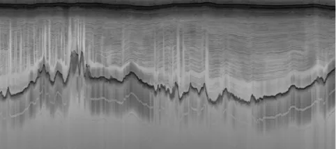
Figure 1 presents an example of an echogram produced by the Multichannel Coherent Radar Depth Sounder System of the Center for Remote Sensing of Ice Sheets (CReSIS) [1]. This echogram is a virtual cross-section of the ice, where the horizontal axis is distance along a flight line and the ver-tical axis is verver-tical distance (depth) from the plane. The echograms reflect a radar’s scattering properties and can be used to estimate an ice sheet’s depth (i.e. the distance from the bedrock to the line near the top of the echogram, which is the ice surface) and the topography of the bedrock beneath the

Fig. 1. Sample radar echogram of an ice sheet, including the surface (very dark line near the top) and bedrock (dark erratic line near the middle) layer boundaries, along with weaker re-turns from contiguous layers of ice between the two.

ice (the dark erratic line near the middle of the figure). These observations can be used as input into glaciological models to forecast ice sheet behavior over time.

Ground-penetrating radar has allowed for data to be col-lected across vast areas of ice, but analyzing it remains a chal-lenge and is typically done by hand. A few recent papers have studied how to use image processing and computer vi-sion techniques to determine layer boundaries automatically or semi-automatically from echograms [2, 3, 4, 5, 6, 7, 8, 9, 10], but this is a hard problem because of the high de-gree of noise, the often faint layer boundaries, and confusing linear structures caused by signal reflections and clutter. In fact, even human annotators produce diverging estimates of the boundaries in many cases. We thus need new techniques which combine together weak image cues, reasoning explic-itly about uncertainty in both the evidence and the resulting layer boundary estimates.

to improve both the accuracy and utility of layer-finding. Our technical innovation uses Gibbs sampling for performing inference instead of the dynamic programming-based solver of [11]. This allows us to strengthen the underlying model and solve for layer boundaries simultaneously, yielding au-tomatic layer detection results that are significantly better than the approach in that paper. Moreover, the Gibbs sam-pler produces explicit confidence intervals, thus giving bands of uncertainty in the layer boundary locations. Since noise and ambiguity in radar echograms are inevitable, we believe that estimating confidence could be crucial in applications of layer identification (e.g. when used as input to glaciological models), and to our knowledge this is the first paper that has demonstrated this capability.

2. RELATED LITERATURE

Several semi-automated and automated methods for identify-ing subsurface features of ice have been introduced in the lit-erature. The most related papers to our work have focused on automated detection in terrestrial echograms. For example, Freeman et al. [6] and Ferro and Bruzzone [4] investigated how shallow ice features can be automatically detected in icy regions on Mars. In other work, Ferro and Bruzzone used echograms of the Martian subsurface to detect basal returns. The subglacial identification problem was studied by Gifford et al [2], who compared two primary approaches, namely an active contour (‘snake’) model and an edge-based technique. Ilisei et al. [5] developed a two-phase technique to exploit the properties of a radar signal for generating a statistical map and applying a segmentation algorithm. Although our application focuses on detecting bedrock and surface layers, other stud-ies use similar techniques to identify internal layers in radar imagery. Approaches include Fahnestock et al. [8], Karlsson and Dahl-Jensen [7], Sime et al. [9], Mitchell et al. [12], and Panton [13].

Our approach is most closely related to Crandall et al. [11], and we use a similar probabilistic framework here. However, our model makes fewer assumptions, our inference algorithm is able to solve for all layer boundaries simultane-ously, and our experiments show a significant improvement in quantitative accuracy compared to ground truth. Addition-ally, our approach is able to characterize uncertainty of the layer boundary estimates by calculating confidence intervals, whereas the technique in [11] simply gives a single layer boundary with no measure of certainty.

3. METHODOLOGY

An echogram is a 2D matrix which represents the scatter-ing properties of the subsurface at each along-track coordi-nate of the radar platform. Figure 1 shows an example of an echogram from the CReSIS dataset [1]. Our task is to find two key features in these echograms: the ice surface boundary (the

strong reflector near the top) and the bedrock boundary (the dark reflector near the middle of the image).

3.1. Modeling layer boundaries

We want to estimate the location of layer boundaries by de-termining their paths through the image. Assume that an echogram has k layer boundaries (with k=2 in our case). Given an echogramIof dimensionm×n, we wish to estimate unknown variablesL={L1, ..., Lk}, whereLi={li1, ..., lin} andlijdenotes the row coordinate of layeriin columnj.

We take advantage of the structure of this problem by pos-ing it as a grid-shaped probabilistic graphical model. In this framework, we are interested in estimatingP(L1, ..., Lk|I), the joint probability over the layer boundaries given the echogram. Unfortunately, this distribution has an alarming dimension of orderO(mkn_{)so that computation and storage} is intractable even for small images. To address this problem, we make three simplifying assumptions: (1) all echograms are equally likely; (2) image characteristics are determined by local layer boundaries; and (3) variables in L exhibit a Markov property with respect to their local neighbors.

Under the first assumption, the joint distribution can be factored into a product according to Bayes’ Law,

P(L1, ..., Lk|I)∝P(I|L1, ..., Lk)P(L1, ..., Lk). (1)

This decomposition reduces the full joint into two intuitive distributions: P(I|L1, ..., Lk) captures how well the im-age data can be explained by a set of layersL1, ..., Lk, and P(L1, ..., Lk)captures prior knowledge about the boundaries, like that they are smooth and do not intersect.

The second assumption implies that parts of the image not near the layer boundaries are generated by noise, so we need only model pixels near boundaries. Thus we can factor P(I|L1, ..., Lk)into a product over layers and columns,

P(I|L1, ...Lk) =

k

Y

i=1

n

Y

j=1

P(I|li,j). (2)

Since boundaries are dark edges, we model the right hand term as a product of gradient magnitude and image intensity,

P(I|li,j)∝ |∇I(li,j, j)| ·(1−I(li,j, j)), (3)

where |∇I(x, y)| is the gradient magnitude at coordinate

(x, y)of the image, and we assume that pixel values have been scaled such thatI(x, y)∈[0,1]. We approximate gradi-ent magnitude using finite differences on a5×5window.

The third assumption simplifies the problem by assuming the graphical model has the property that each nodeli,jis in-dependent of the remaining variables inLgiven its immediate neighbors in the graph. Under this assumption, we have,

P(L1, ..., Lk)∝

k

Y

i=1

n

Y

j=1

whereN(li,j)is the set of directly connected nodes in the graph (i.e.N(li,j) ={la,b|1 =|a−i|and1 =|b−j|}). We defineP(li,j|N(li,j))as the product of independent vertical and horizontal components. Along the same layer, li’s are encouraged to be smooth by a zero-mean Gaussian which is truncated to zero outside a fixed interval,

P(li,j|li,j−1)∝

N(li,j−li,j−1; 0, σ) |li,j−li,j−1|< φH

0 otherwise,

(5) while a step function encourages layers not to overlap,

P(li,j|li−1,j)∝







0 li,j ≤li−1,j

0.1 li,j−li−1,j < φV

1 otherwise.

(6)

This model is similar to [11] but with important improve-ments. In [11], the vertical pairwise potentials are zero at and above intersection points and uniform elsewhere. But it is common in this data to see radar reflections of the sur-face layer directly below the actual sursur-face, so we add a fixed-width low probability region directly below them to reduce false bedrock detections on these reflections. Perhaps more importantly, the model in [11] breaks these vertical constraints in order to simplify inference by greedily solving each layer conditioned on the previous one. We avoid doing this, and our experiments show that this holistic inference approach offers substantial improvement in accuracy.

3.2. Statistical inference

The model defined by equations (1), (2), and (4) is a first-order Markov Random Field. Unfortunately, finding the val-ues ofLthat maximizes equation (1) is NP-hard in the general case [14]. Rather than trying to solve this as an optimization problem, we instead attempt to estimate functionals of the full joint distribution via Gibbs sampling.

Gibbs sampling is a Markov Chain Monte Carlo (MCMC) method which is capable of producing samplesX(1)_{, ..., X}(J)

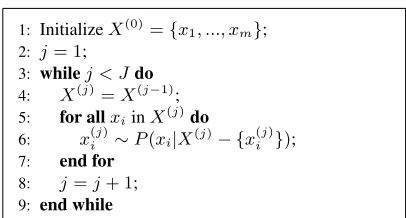
from a distributionf(x)without requiring the ability to di-rectly sample or even know the form off(x)[15]. This is ac-complished by iteratively sampling each variable conditioned on the remaining variables. Pseudo-code for Gibbs sampling is shown in Figure 2. This sampler provides a flexible frame-work for generating samples of a complex distribution, as-suming samples can be taken from usually simpler full con-ditionals. The run-time complexity isO(mJ), but in practice depends on the ease of sampling from the full conditionals.

It can be shown via Bayes Law and the independence as-sumptions in equations (2) and (4) that the full conditionals for eachlij can be computed easily,

P(lij|I, N(lij)) =P(I|lij)P(lij|N(lij)). (7)

As the domain oflijis discrete and finite, sampling from this conditional is well-defined. As an additional optimization, we

1: InitializeX(0)={x1, ..., xm}; 2: j= 1;

3: whilej < Jdo 4: X(j)_=X(j−1)

; 5: for allxiinX(j)do 6: x(_ij)∼P(xi|X(j)− {x

(j)

i }); 7: end for

8: j=j+ 1; 9: end while

Fig. 2. General algorithm for Gibbs sampling.

make use of the vertical and horizontal thresholds in equa-tion (6) to sparsify the computaequa-tion of P(lij|N(lij)), since most entries are known to be zero. We apply the Gibbs sam-pler to generate a sequence of samplesL(B), ..., L(J)where Bis a burn-in time during which samples are discarded. This is a common practice with MCMC methods to reduce sensi-tivity to initial values. To predict the layer locations we take the mean of ourM = J −B samples, which approximates the expectation of the joint distribution for largeM,

E[P(L1, ..., Lk|I)] = lim M→∞

1

M

X

L(i).

To produce confidence intervals around this mean, we use the fact that the marginal distribution of a variable can be esti-mated by discarding other variables in the sample, and take the 2.5% and 97.5% quantiles.

4. EXPERIMENTAL RESULTS

We tested our layer-finding approach using a set of 826 pub-licly available radar echograms from the 2009 NASA Oper-ation Ice Bridge program, collected with the airborne Multi-channel Coherent Radar Depth Sounder system of [1]. Each echogram has a resolution of 700 by 900 pixels (where 900 pixels represents about 30km of data on the horizontal axis, and 700 pixels corresponds to 0-4km of ice thickness on the vertical axis). This dataset was used by [11] so we can di-rectly compare the accuracy of the two techniques, and we used the source code provided by the authors.

The images have ground-truth labels produced by human annotators, but these labels are often quite noisy. For instance, sometimes the annotators could not find a reasonable layer boundary and simply “gave up” by not marking anything at all. To decouple the error in the ground-truth from the method evaluation, we removed images with incomplete ground truth (including those with partially defined layers and those with less than two layer boundaries). We ran our method on the remaining 560 images. For each image, we collected 10,000 samples after a burn-in period ofB=20,000 iterations.

Ground truth Result of [11]

Our solution with 95% confidence intervals

Ground truth Result of [11]

Our solution with 95% confidence intervals

Ground truth Result of [11]

Our solution with 95% confidence intervals

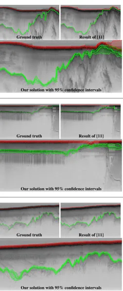
Fig. 3. Results on three sample echograms. Each pane in-cludes the hand-labeled ground truth image(top-left), the out-put of [11](top-right), and then our output(bottom). Best viewed in color.

Mean Error Median Mean Error Approach Surface Bedrock Surface Bedrock

[11] 22.3 43.1 10.6 14.4

Ours 9.3 37.4 5.9 9.1

Table 1. Evaluation of our method on the test set. Error is measured in terms of absolute column-wise difference com-pared to ground truth, summarized with average mean devia-tion and median mean deviadevia-tion across images, in pixels.

of [11]. We present quantitative performance metrics in Ta-ble 1. We measure accuracy by viewing ground truth and es-timated layer boundaries as 1-D signals, and computing the mean absolute deviation (in pixels) between the two. We use two summary statistics: mean column-wise absolute error over all images and the median of the column-wise mean ab-solute errors across images. The first measures how well pre-dicted layers match the ground truth, treating columns within an image as uncorrelated, while the later metric recognizes that high error in one column in an image is highly correlated with the error in the remaining columns and looks at error from a per-image viewpoint. Under both metrics, we outper-form the method of [11] significantly, by decreasing the error rate by about 44.3% for surface boundaries and 48.3% for bedrock. Our technique is slower than [11] (about 17 seconds per image), but since layer finding is trivially parallelizable across images, we believe accuracy is much more important than compute time in practice.

We also quantified how informative the confidence inter-vals are by computing the percentage of ground truth layer points that are contained within the estimated intervals. We found that 94.7% of the surface boundaries and 78.1% of the bedrock boundaries are within the intervals, for an overall per-centage of 86.4%. The fact that this number is close to but less than 95% reflects that our framework is a good but not perfect model of layers in echogram images.

5. CONCLUSION

We proposed an automated approach to estimate bedrock and surface layers in multichannel coherent radar imagery and demonstrated its effectiveness on a real-world dataset against the state-of-the-art. Our technique also produces confidence interval estimates and we evaluated their correctness. We be-lieve layer-finders that provide such confidences may improve climate models by quantifying error in the input data.

6. ACKNOWLEDGMENTS

7. REFERENCES

[1] C. Allen, L. Shi, R. Hale, C. Leuschen, J. Paden, B. Pazer, E. Arnold, W. Blake, F. Rodriguez-Morales, J. Ledford, et al., “Antarctic ice depthsounding radar instrumentation for the NASA DC-8,” IEEE Aerospace and Electronic Systems Magazine, vol. 27, no. 3, pp. 4– 20, 2012.

[2] C. Gifford, G. Finyom, M. Jefferson, M. Reid, E. Akers, and A. Agah, “Automated polar ice thickness estima-tion from radar imagery,” IEEE Transactions on Image Processing, vol. 19, no. 9, pp. 2456–2469, 2010.

[3] A. Ferro and L. Bruzzone, “Analysis of radar sounder signals for the automatic detection and characterization of subsurface features,” IEEE Transactions on Geo-science and Remote Sensing, 2012.

[4] A. Ferro and L. Bruzzone, “Automatic extraction and analysis of ice layering in radar sounder data,” IEEE Transactions on Geoscience and Remote Sensing, 2013.

[5] A.-M. Ilisei, A. Ferro, and L. Bruzzone, “A tech-nique for the automatic estimation of ice thickness and bedrock properties from radar sounder data acquired at Antarctica,” inIEEE International Geoscience and Re-mote Sensing Symposium, 2012, pp. 4457–4460.

[6] G. Freeman, A. Bovik, and J. Holt, “Automated detec-tion of near surface Martian ice layers in orbital radar data,” inIEEE Southwest Symposium on Image Analy-sis & Interpretation, 2010, pp. 117–120.

[7] N. Karlsson, D. Dahl-Jensen, S. P. Gogineni, and J. D. Paden, “Tracing the depth of the holocene ice in north greenland from radio-echo sounding data,” Annals of Glaciology, 2012.

[8] M. Fahnestock, W. Abdalati, S. Luo, and S. Gogineni, “Internal layer tracing and age-depth-accumulation rela-tionships for the northern greenland ice sheet,” Journal of Geophysical Research, vol. 106, no. D24, pp. 33789– 33, 2001.

[9] L. Sime, R. Hindmarsh, and H. Corr, “Instruments and methods automated processing to derive dip angles of englacial radar reflectors in ice sheets,” Journal of Glaciology, vol. 57, no. 202, pp. 260–266, 2011.

[10] J. Mitchell, D. Crandall, G. Fox, M. Rahnemoonfar, and J. Paden, “A semi-automatic approach for estimating bedrock and surface layers from multichannel coherent radar depth sounder imagery,” inSPIE Conference on Remote Sensing, 2013.

[11] D. Crandall, G. Fox, and J. Paden, “Layer-finding in radar echograms using probabilistic graphical mod-els,” inInternational Conference on Pattern Recogni-tion, 2012, pp. 1530–1533.

[12] J. Mitchell, D. Crandall, G. Fox, and J. Paden, “A semi-automatic approach for estimating near surface internal layers from snow radar imagery,” inIEEE International Geoscience and Remote Sensing Symposium, 2013.

[13] Christian Panton, “Automated mapping of local layer slope and tracing of internal layers in radio echograms,”

Annals of Glaciology, vol. 55, no. 67, pp. 71–77, 2014.

[14] Daphne Koller and Nir Friedman, Probabilistic graph-ical models: principles and techniques, MIT Press, 2009.