3 D sensing of object orientation using back propagation neural network

3-D Sensing of Object Orientation

using

Back Propagation Neural Network

Muhammad Dimyati bin Abdullah

A thesis submitted in partial fulfilment of the requirements for the Master of Technology program in Information Technology

in

Department of Electrical & Electronic Engineering University of Tasmania

Australia

Supervisor

Abstract

This thesis is about the application of Neural Networks in the sensing of an object position relative to a reference point. An object is rotated a certain angle in space and a Neural Network was then used to estimate its orientation. Previous methods had always been to transform 3-dimensional data into 2-dimensional data before presenting it to the network. In this thesis 3-dimensional data is used as the input to the Neural Network.

Acknowledgment

Firstly I would like to thank my supervisor Professor D. T. Nguyen for his guidance and assistance in order for me to pursue this very interesting subject. I would also like to thank Dr. D. H. Lewis who is the course coordinator.

I am also indebted to my wife who has been most understanding and helpful during the duration of the course, and to my children who are a source of joy and purpose in times of difficulties.

Table of Contents Page

1 Introduction 1

2 Object Recognition 4

2.1 2-D Vision 4

2.2 3-D Vision 7

2.3 Tactile Sensing 8

3 Artificial Neural Network

3.1 Introduction 12

3.2 Classification of Neural Networks 14 3.3 The Back Propagation Neural Network 16

3.4 Network Dynamics 17

3.5 The Learning Parameters 19

4 Graphic Transformation

4.1 Using Autocad 21

4.2 3-D Graphic Program 21

4.3 The Transformation Matrix 22

5 Simulations 26

6 Results and Discussions 28

7 Conclusions 43

Chapter 1

INTRODUCTION

The determination of an Object Orientation or Object Pose Estimation is currently being investigated in the realm of computer vision systems by researchers such as T.Poggio and S. Edelman[1], B.Wirtz and C.Maggioni[2], M.W. Wright and F. Fallside[3] who have obtained results which show that the recovery of an object pose was possible when using Artificial Neural Network(ANN) such as the Radial Basis Function, Kohonen and Back Propagation. However in all the three research works carried out, 3- D data was all transformed into 2-D data before being presented to their respective ANNs. In the field of machine vision the determination of an object pose plays an important part in object recognition.

With the combination of 2-D vision and 3-D data we can perhaps make the process of QC more efficient in selecting or rejecting a particular product.

If a particular computer vision system can recognise an object in 2-D vision as well as correlating it with 3-D data then the system will be a much robust one. In the field of speech recognition integration of visual and auditory speech signals [4] it was shown that better results were obtained when they were fused together compared to if they were used on their own. Perhaps this can give us a guideline in the fusion of 3-D data with 2-D image in order obtaining a much improved computer vision system.

This thesis is about the use of an Artificial Neural Network to sense an object's position using 3-D input data where the output data is the angle of rotation about the X, Y and Z-axis through which the object had been rotated. The simple Backpropagation Neural Network was used in conjunction with a • CAD system to demonstrate the capability of the ANN to recognise and sense object position when presented with 3-D data. It will also attempt to show the ability of the Back Propagation ANN to identify the object even if there are certain hidden surfaces.

Chapter 2

OBJECT RECOGNITION

In the field of robotics object recognition is a precursor to many other important robotic tasks, including grasping, manipulation, assembly and inspection. Before attempting such complex robotic tasks, there is the need to be able to correctly recognise the relevant objects with respect to its surrounding in the first place. Object recognition also means understanding an object's position and orientation in space in a viewpoint-independent manner [5].

The following sections present some of the techniques used in object recognition, which include vision only system, range scanning and tactile sensing.

2.1 2-D VISION

and Hildreth[6] has also tried to isolate those parts of human visual information processing that seem to operate independently.

Stages used in machine vision usually involve image acquisition using static images with the object being carefully illuminated. The process of thresholding is then made to manipulate the grey level, thus establishing a clear contrast upon the image in order to establish gradients for the object's contour. This process also produce a binary image. The next step is edge detection by convolving the image with the Laplacian of a Gaussian, also known as Marr-Hildreth edge detection operator[6]. This process is usually a computationally burdensome process. A chain coding process is then made in order to obtain the perimeter(p) of the object as well as determining its area(A). The ratio of p2/A is obtained and compared to existing database. If similar ratio value exist in the database then the object is identified. Other techniques being tried are segmentation and region analysis.

space curves and regions obtained via the methods mentioned above are then matched with one of these views. Fisher[8] used an approach in which certain weak constraints about a surface's images over different viewpoints were computed to aid in determining the object's position and orientation.

Image space matching is not powerful because it loses the inherent sense of the 3-D object to be recognised. The projective space approach fails to maintain the consistent structure of an object across the many possible visual interpretations. The question of "How many characteristic views of an object are sufficient?" is open; clearly the answer is many. Establishing a metric on this kind of matching is difficult especially if the sensed view is between two stored views. Therefore 2-D projective invariants are still weak, and are not robust enough to support consistent matching over all viewpoints.

While some progress has been made, the state of machine vision is still primitive. Most commercial machine vision systems available today use simple template matching of the 2-D silhouettes. Recently some application with the use of ANN in machine vision had begun to be available commercially [9]

2.2 3

D VISION

At present most machine vision works are centred on the problem of obtaining depth and surface orientation from an image. 3-D data acquisition must cover a wide spectrum of needs, for example, the detailed shape Of an object in the scene might be needed instead of the mere range value of its surface elements. If a full 3-D description is required, view integration must be performed on multiple partial views of the object. In some cases, sparse 3-D data is all that is needed to understand a scene, however, in numerous applications, the 3-D structure of the scene must be known and a 3-D range sensing method must be implemented.

These methods are usually concerned with the recovery of surface orientation from one or multiple grey-level pictures.

Most active ranging techniques have little to do with the human visual system. Their purpose is neither to model nor to imitate biological processes but rather to provide an accurate range image to be used in a given application involving 3-D operations. Active techniques include Striped Lighting and Active Stereo, Moire Shadows, Laser or Ultrasonic Time-of-Right Techniques, Conventional or Synchronised Triangulation Range finder, Range from defocusing and Intensity-Guided Rangefuider.

Problems of using range sensing technique are the potentially hazardous nature of some of the methods using laser imaging. In Photometric stereo, great demands are made on the illumination of the scene and on proper understanding of the reflectance properties of the objects to be viewed. All the rangefulder techniques mentioned above face the same major problem: the 3-D data provided conveys information only for the "visible' part of the scene. If a full 3-D image of an object is required, several images must be acquired from different positions and view integration must be performed.

2.3 TACTILE SENSING

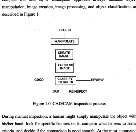
complex the task is, a conceptual approach always includes object manipulation, image creation, image processing, and object classification, as described in Figure 1.

OBJECT

MANIPULATE

CREATE IMAGE

PROCESS IMAGE

CLASSIFY

RESULTS REVIEW GOOD

BAD REINSPECT

Figure 1.0 CAD/CAM inspection process

During manual inspection, a human might simply manipulate the object with his/her hand, look for specific features on it, compare what he sees to some criteria, and decide if the comparison is good enough. At the most automated levels, there is no human interaction. A robot places the object in a system with some sensing mechanism, a computer automatically initiates imaging and constructs an image from the sensor output, and the computer logic processes the image data and classifies the object as good or bad.

sensing is like imitating the human fingers in manipulating the object; similiarly machine vision is like trying to imitate the vision of a human.

Tactile sensing using a Coordinate Measuring Machine can be used to acquire 3-D data of an object. These sensors vary in their ability to sense a surface, at the lowest level, simple binary contact sensor such as microswitches report 3- D coordinates of a contact point. In fact this method is being used extensively in industry in the process called reverse engineering. In this process a sensor traces the surface of the components to be copied. The 3-D data obtained is stored in a database. A similar component can then be machined out of the collected data.

The next level of tactile sensor reports grey values that are proportional to the force or displacement of the sensor. The most capable of these sensors can also sense surface orientation, returning a surface normal vector.

Chapter 3

ARTIFICIAL NEURAL NETWORKS

3.1 INTRODUCTION

An Artificial Neural Network is a massively interconnected network of a large numbers of processing elements, called neurons or nodes. A neuron receives input stimuli from other neurons if they are connected to it or/and the external world. A neuron can have several inputs, but has only one output. This output however can be routed to the inputs of several other neurons. Each neuron has certain constant parameters associated with it. These are its threshold, transfer function and weights associated with its inputs. Each neuron performs a very simple arithmetic operation, i.e. it computes the weighted sum of its inputs, subtracts its threshold from the sum, and passes the result through its transfer function. The output of the neuron is the result obtained fom this function. The output of the neuron is therefore a mathematical function of its input and can be expressed as

y =

f(

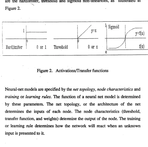
are the hardlimiter, threshold and sigmoid non-linearities, as illustrated in Figure 2.

Haraniter

0 or 1 Threshold

Figure 2. Activations/Transfer functions

Neural-net models are specified by the net topology, node characteristics and training or learning rules. The function of a neural net model is determined by these parameters. The net topology, or the architecture of the net determines the inputs of each node. The node characteristics (threshold, transfer function, and weights) determine the output of the node. The training or learning rule determines how the network will react when an unknown input is presented to it.

called learning. If the desired result is given to the net, the learning is supervised. If it is not, the learning is unsupervised.

A second characteristic that makes ANN superior to other recognition systems is its ability to tolerate noise in an input pattern. If a net has been trained sufficiently, it is capable of performing well even if input patterns are noisy or incomplete.

Another important aspect of ANNs which is of importance to this thesis is their ability to fuse information together in an optimal way. This ability can overcome the problem of integrating multiple views in object recognition as well as fusing different information collected from a multisensor system.

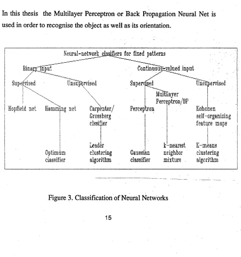
3.2 CLASSIFICATION OF NEURAL NETS

Figure 3 shows a taxonomy of six important neural nets used for classification of static input patterns. Nets can have either binary or continuous valued inputs. Binary inputs take on one of two possible values, while continous-valued inputs can take on any value in a specified range.

input

Sup erldied

Ilditlayer

Pero eptron/BP

Perceptrou

k -nearest

neighbor

mixture .

Gaus

classifier

Trik-pervised

weights are changed as a function of the difference between the outputs. Examples are the Hopfield net[12] and the Hamming net[12] with binary inputs, and the Back Propagation/Multilayer perceptron with continuous inputs. For the unsupervised training, no information concerning the correct output is provided to the net. The net constructs an internal model that captures regularities in input training pattern. In other words, the net forms its own exemplars(during training) by clustering input patterns which are similar to each other within a specified tolerance. Kohonen's feature-map-forming nets [12] are examples of this type of net.

In this thesis the Multilayer Perceptron or Back Propagation Neural Net is used in order to recognise the object as well as its orientation.

Neural-network dadfiers for fixed pathrus

____---

llinamilifil

...-

Supefyised Una frA rvis ed

_,..

\

---____.

Hopfield net HamMing net Carii

\

en

Gros s b erg

dm ier

9

Leader

Optimum clustering

classifier algorithm

self -organizing

feature maps

-

K-means

clustering

algorithm •

••:,,

•

; • •

, .•__

• • „

11

Output. Array

Hidden

Layer 1:

„ ; Hidden Layer

Hidden Lay

47,11

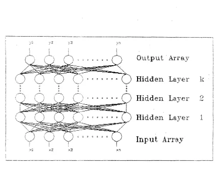
3.3 THE BACK PROPAGATION NEURAL NETWORK

The Back Propagation(BP) network consists of input layer, hidden layerls and an output layer, each layer however may contain a different number of nodes. The BP network is a supervised network where input as well as output sets of training vectors have to be presented to it for training purposes. Every node in the output layer is connected to every unit in the input layer. Figure 4 shows an example of a BP network.

;

7

Input Array

n

The output generated by the network is compared with the target output. The difference between output and target is the error signals which is then back propagated into the network and the corresponding weight changes at various nodes are then made until the output of the network is similar to the target output. Thus, a Back Propagation network learns a mapping function by repeatedly presenting patterns from a training set and adjusting the weights. Each pass through the training set is called a cycle.

Input patterns that are similar to each other produce output patterns that are similar because of the direct mapping of inputs to outputs in a two-layer network. A two-layer network cannot learn the exclusive-OR functions, therefore in order to learn any arbitrary mapping the network must have at least three layers.

3.4 NETWORK DYNAMICS

0.50

0.25 —

Activation — (loci-

-0.25 -

-0.50 1 I I If I I I I I I I I 7 -6 -5 -4 -3 -2 -1 0 1 23 4 567

Net Input 1) Apply an input vector and calculate the output Y.

2) Calculate the weight changes using the equation below:

8j = ( - Aw . . = _{.11 J}

where Awji is the correction associated with the weight from the ith neuron in the input layer to the jth neuron in the output layer. Oi is the ith component of the input vector and is r the "learning rate" which controls the size of the weight changes.

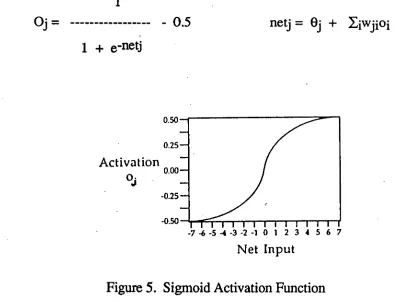
The Back Propagation activation used in this thesis is the sigmoid activation function as shown in Figure 5.

1

Oj 0.5 netj = Oi + Eiwijoi

1

e

netj

Neti is the sigmoid activation function used to modify each weight, Oi is the

bias for unit j. The biases are also learned in the same manner in which the

weights are learned. Unit activations range from -0.5 to 0.5, and networks

learn more quickly if the input patterns are scaled in this range.

The GDR guarantees a steepest gradient descent in the total root mean

square(RMS) error. This measure is computed by summing the squares of the

target minus the output for every output unit and for every pattern, averaging

this, then taking the square-root as shown in the expression below:

_ )2

Total RMS error =

# patterns x # output units

where p is the pattern, o is the output unit, and t is the target output unit.

3.5 THE LEARNING PARAMETERS

tiny solution regions, thus requiring a small 11 or less, and require many learning cycles. In order to increase learning rate a momentum term a [13] is added so as not to make RMS oscillate. The momentum term determines what portion of the previous weight changes will be added to the current weight changes. The total weight change equation then becomes:

Awii(t+1) = ii(8joi) aAwii(t)

where i(Sjoi) is the current weight change dictated by the GDR. In practice, the value of ₁ and a are always adjusted until the total RMS error display shows a generally decreasing value with time.

Chapter 4

GRAPHICAL TRANSFORMATION

4.1 USING AUTOCAD

A 3-D object was created using AUTOCAD®[1 4] and stored in the computer, the object can be manipulated to rotate about X, Y or Z axis. For every new position the vertices of the object were recorded using the INQUIRY command of the CAD program. It was also possible to have a solid view of the object instead of a wireframe drawing using the HIDE command which removed hidden lines in the drawing.

4.2 3

0 GRAPHIC PROGRAM

angles, if we are looking along the positive half of the axis toward the coordinate origin. The Pascal program is in Appendix B.

4.3 THE TRANSFORMATION MATRIX

For the rotation about X, Y and Z axis the coordinates of the vertices are submitted to the following transformations matrix;

10 0 0

Rx = 0 cos° sine 0

0 -sine cos0 0

0

O.

cos0 0 -sine 0

Ry = 0 1 0 0

sine 0 cos° 0

000 1

.0111111.

cose sine 0 0

Rz = -sine cos° 0 0

00 1 0

0 0 0 1

_)

Translation of the coordinates is specified by the following matrix

1

TL= 0100

0 0 1 0

In order to visualise the shape of the object, lines are drawn connecting all the vertices, however these lines are not being used as part of the training set for the Neural Network. The Turbo Pascal program was used to generate the coordinates for various positions of the object. This values were then cross-checked with those values obtained using Autocad.

A problem of using 3-D data is the amount of transformation that must be undertaken in order to rotate the various vertices about the X,Y and Z-axis. If the object is rotated about an arbitrary axis where the specifications for the rotation axis and rotation angle are given, then the transformation procedure is as follows:

1. Translate the object so that the rotation axis passes through the coordinate origin.

Rotate the object so that the axis of rotation coincides with one of the coordinate axes.

3. Perform the specified rotation.

Apply inverse rotations to bring the rotation axis back to it original orientation.

5. Apply the inverse translation to bring the rotation axis back to its original position.

Therefore the complete transformation is as follows;

However in this thesis the rotation of the object was made about it centre of gravity which acted as the point of coordinate origin, thus eliminating the need to translate or inverse translate the object. Therefore the only transformations needed are as follows:

[ x, y, z]' = Rz.Ry.Rz.[ x, y, z]

N

_N

_N

N

Figure 6. Wireframe drawing

Chapter 5

SIMULATIONS

Simulations were carried out for two cases; the first one was concerned with the use of 3-D data of the object vertices' coordinates for a variety of poses. The first set of 3-D data were simulated as though it was obtained via a tactile sensing mechanism and the problems of hidden vertices were therefore eliminated. The input values for the Back Propagation network were the various vertices' coordinates and the target values are the rotational parameters. Since the object can assume a large number of positions in space, the rotational parameter were limited between 0 - 30 degrees with 5_degree intervals for all axes. The training data set(SET12345.DAT) and the test data set(TESTDATA.DAT) that were used are in Appendix A. The first BP network is called NET 1.

set(H1DEDATA.DAT) for these are in Appendix A, and the second BP network is called NET2.

The second simulation also simulates how 3-D data obtained by tactile sensing can be integrated with another set of 3-D data obtained through 3-D vision system. This is assumes that the vision system is viewing from a fixed point, therefore there is a possibility that it cannot detect hidden vertices.

All the data were normalised between 0.5 and -0.5. This setting was recommended by the maker of the Back Propagation Network network software being used ie. ANSIM® [15]. The target outputs are the ratio of (angle of rotation)/360. Damaged weights were set between 0.5 to -0.5, learning rate was set at 0.1 and the momentum was set at 0.6, however these values were occasionally changed in order to speed up training or to reduce the RMS error fluctuation. Training

was

49 nodes.

diskettes enclosed

All the training data needed to

be processed

data, such as those which had the same

Chapter 6

RESULTS AND DISCUSSIONS

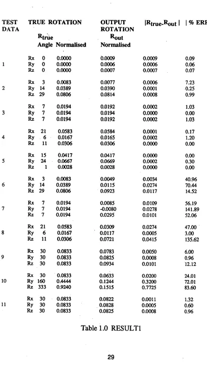
For the first simulations using NET1, the test data TESTDATA.DAT is used. The results are illustrated in Figure 8 to Figure 15 as well as in Table

1.0.

Figure 8 uses test data 11 which is part of the training data set. As expected the output position(Rout) produced by the network is very close to the target value(Rtrue). Figure 8 shows that the output image is superimposed upon the target image. The image of the car that is lying parallel to the Y-axis serves as a reference position as well as the

initial

However test data 2 and 4 are not

the

lie within

when test data

its

TEST DATA TRUE ROTATION Rtrtie Angle Normalised OUTPUT ROTATION Rout Normalised

IRtrue-Rout I I % ERROR I

Rx 0 0.0000 0.0009 0.0009 0.09

1 Ry 0 0.0000 0.0006 0.0006 0.06

Rz 0 0.0000 0.0007 0.0007 0.07

Rx 3 0.0083 0.0077 0.0006 7.23

2 Ry 14 0.0389 0.0390 0.0001 0.25

Rz 29 0.0806 0.0814 0.0008 0.99

Rx 7 0.0194 0.0192 0.0002 1.03

3 Ry 7 0.0194 0.0194 0.0000 0.00

Rz 7 0.0194 0.0192 0.0002 1.03

Rx 21 0.0583 0.0584 0.0001 0.17

4 Ry 6 0.0167 0.0165 0.0002 1.20

Rz 11 0.0306 0.0306 0.0000 0.00

Rx 15 0.0417 0.0417 0.0000 0.00

5 Ry 24 0.0667 0.0669 0.0002 0.30

Rz 1 0.0028 0.0028 0.0000 0.00

RX 3 0.0083 0.0049 0.0034 40.96

6 Ry 14 0.0389 0.0115 0.0274 70.44

Rz 29 0.0806 0.0923 0.0117 14.52

Rx 7 0.0194 0.0085 0.0109 56.19

7 Ry 7 0.0194 -0.0080 0.0278 141.89

Rz 7 0.0194 0.0295 0.0101 52.06

Rx 21 0.0583 0.0309 0.0274 47.00

8 Ry 6 0.0167 0.0117 0.0005 3.00

Rz 11 0.0306 0.0721 0.0415 135.62

Rx 30 0.0833 0.0783 0.0050 6.00

Ry 30 0.0833 0.0825 0.0008 0.96

Rz 30 0.0833 0.0934 0.0101 12.12

Rx 30 0.0833 0.0633 0.0200 24.01

10 Ry 160 0.4444 0.1244 0.3200 72.01

Rz 333 0.9240 0.1515 0.7725 83.60

Rx 30 0.0833 0.0822 0.0011 1.32

11 Ry 30 0.0833 0.0828 0.0005 0.60

Rz 30 0.0833 0.0825 0.0008 0.96

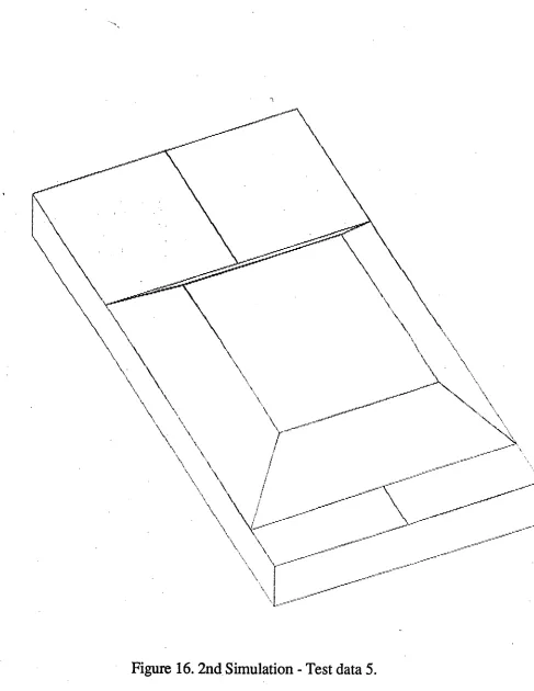
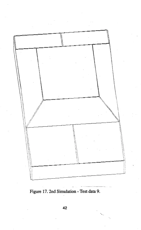
above the percentage error is quite high, however looking at it in Figure 11 and 12 the total deviation is not very large, especially the one in Figure 11.

Test data 9 uses test data 11 which is part of the training data set. However test data 9 had 3 set of corrupted vertices' coordinates. From table 1.0 above as well as Figure 13 it can be shown that NET1 still manage to estimate the position of the car image. The percentage error is also significantly smaller than that obtained when using data 6 and 8.

Figure 14 shows the result of using a test data which does not lie within the training data set, therefore the network fails to identify its position. For test data 7, even though the percentage error is very high, the deviation observed in Figure 15 is not as drastic as that in Figure 14.

Generally speaking NET1 is able to identify correctly all the 3-D test data sets which were presented to it, provided these data sets were not corrupted and lay within the preset limits.

C) C) 01 Cr) Cr)

e• Lr7 co _•

. •

•-:, 3 '

....'s _-... ?

:.

•

• ,.„

•, • •S

s s, i

"?"‘

Ni

• 0°)

v-I N-1 •

Cr)

%.1:1 itr

9£

LA.) k•O CO

• - • cr.

N C) LO

, ••

„

SN

...;.%

v • •

• • _• •

S.

• • _{• •}

'sse„

•„.

, •

1

C.,

•

4ç '4,

•

1 '4,

•

...• ..••• •

tk,

„

Cr) CO Tr'

TV r,- 1.11

C) CO • • •

I 1 I $$$$$ •

kr,, \ k '''.•• / ‘ .'

.t. .. .. ... A ... ... ... ... 1 '

1 k ‘ ; . N ;'‘ •! :•• 1 ,

k t. Zt '' ' \ \ • k .... i k

4. 0. ,.. ,. k.

“ k 1, 0

...

) It

A 1 i' ' _k k _i t ‘ ' :

k.

, ,,

'½

‘1 ‘ i i 4

' \ ii ' i i, ':;.** 1 \

i 't 4 t

i 1 Z \ i. '4. • 't k

•% : Z k

• ..,...•..•..•.• .

‘ \ %

.' '

Is ki • .. ' .'... ' ., .;, ‘ \ • 1 ,

Table 2 presents the results obtained after using the test data HIDEDATA.DAT for NET2.

TEST TRUE ROTATION OUTPUT Rtrue-Rout I % ERROR I

DATA ROTATION

Rtrue Rout

Angle Normalised Normalised

1 Rz 0 -0.5000 -0.4977 0.0023 0.46

2 Rz 30 -0.4167 -0.4167 0.0000 0.00

3 Rz 80 -0.2778 -0.2779 0.0001 0.04

4 Rz 120 -0.1667 -0.1665 0.0002 0.12

5 Rz 160 -0.0556 -0.0554 0.0002 0.36

6 Rz 200 0.0556 0.0555 0.0001 0.18

7 Rz 240 0.1667 0.1668 0.0001 0.06

8 Rz 280 0.2778 0.2780 0.0002 0.08

Rz 320 0.3889 0.3908 0.0019 0.49

Table 2 RESULT2

Chapter 7

CONCLUSIONS

From the results obtained in the simulations, the following conclusions can be drawn;

* The Back Propagation neural network is able to learn to estimate the pose of an object relative to a standard view using 3-D data.

* The integration of full 3-D data plus data having some hidden vertices makes the Network more accurate in estimating object position.

* The fusion of 3-D data obtained different sensors is possible using Neural Network thus making the object recognition system more robust.

The technique used in this thesis does have its limitations such as;

* To estimate the pose position for the entire viewing sphere a large training data set had to be produced. Since this thesis used a

Preprocessing of the solid model feature is a necessary step before presenting it to the network. This involves a tedious cross-checking of training data( in order to root out repeated data sets and contradicting data sets) and the determination of hidden vertices.

References

1. T.Poggio and S. Edelman, "A network that learns to recognise three-dimensional objects," NATURE 343:263-266, 18 Jan. 1990.

2. B. Wirtz and C. Maggioni, " 3D-Pose Estimation by an Improved Kohonen net.," International Workshop on Visual Form, Capri. Plenum

press,

3. M.W. Wright and F. Fallside, " Object Pose Estimation by Neural Network," University of Cambridge, UK.

4. Ben P. Yuhas, Moise H. Goldstein, Jr, and Terrence J. Sejnowski, "Integration of Acoustic and Visual Speech Signals Using Neural Networks," IEEE Communications Magazine - Nov. 1989 pp. 65-71.

5. Peter K. Allen, "Robotic Object Recognition Using Vision and Touch," Kluwer Academic Publishers - 1987, pp. 4

6. David Marr and Hildreth, "Theory of Edge detection," Proc. Royal Society of London Bulletin, Vol. 204, pp. 301-328, 1979.

7. Oshima, M. and Y. Shiraj, "Object recognition using three dimensional information," IEEE trans. on Pattern Analysis and Machine Intelligence, Vol. PAMI-5, no. 4, pp. 353-361, July 1983

8. Fisher, R.

B, "

9. "Neural Computing from laboratory into industry," The Journal of the Instituition of Engineers Australia Vol 6 No 9, 15 May 1992 pp.16 -18.

11. Kinoshita, ,G., S. Aida and M. Mori, " A pattern cassification by dynamic tactile sense information processing," Pattern Recognition, vol. 7, pp.243-250, 1975. Extracted from "Robotic Object Recognition Using Vision and Touch," by Peter K. Allen, Kluwer Academic Publishers - 1987, pp. 64-65.

12. Richard p. Lippmann, "An introduction to computing with Neural Nets," IEEE ASSP magazine, Vol 4, No. 2, April 1987.

13. J. L McClelland and D.E. Rummelhart, "Explorations in Parallel Distributed Processing," MIT Press, 1988.

14. AUTOCAD - Copyright (C) Autodesk, Inc.

Appendix A

Due to the large amount of training data sets and test data sets, the

print out will be more than a hundred pages. In order to save time

and effort all the following informations are available in the

enclosed diskette.

SIMULATION I

Training data sets text form Training data sets data form Trained BP network program Test data sets

Results of Simulation I

SET12345.TXT SET12345.DAT NET1

TESTDATA.TXT RESULT1.TXT

SIMULATION II Filename

Training data sets text form Training data sets data form Trained

BP

Results of Simulation II

HIDE15.TXT

HIDE15.DAT

NET2.NET

TESTDATA.TXT

TRAIN 3, 16, 3, 1

/* Input vector 1: */ -0.125000, -0.300000, -0.050000,

-0.125000, 0.200000, -0.050000, 0.125000, 0.200000, -0.050000, 0.125000, -0.300000, -0.050000, -0.125000, -0.300000, 0.000000, -0.125000, -0.150000, 0.000000, -0.125000, 0.150000, 0.000000, -0.125000, 0.200000, 0.000000, 0.125000, 0.200000, 0.000000, 0.125000, 0.150000, 0.000000, 0.125000, -0.150000, 0.000000, 0.125000, -0.300000, 0.000000, -0.075000, -0.100000,0.050000,

-0.075000, 0.100000, 0.050000, 0.075000, 0.100000, 0.050000, 0.075000, -0.100000, 0.050000,

/* Output vector 1: */ 0.000000, 0.000000, 0.000000,

/* Input vector 2: */ -0.245300, -0.209500, =0.063500,

0.002300, 0.224100, -0.088800, 0.214400, 0.106500, -0.028400, -0.033200, -0.327100, -0.003000, -0.254600, -0.201400, -0.015000, -0.180400, -0.071300, -0.022600, -0.031800, 0.188900, -0.037900, -0.007000, 0.232300, -0.040400, 0.205100, 0.114700, 0.020100, 0.180400, 0.071300, 0.022600, 0.031800, -0.188900, 0.037900, -0.042500, -0.319000, 0.045500, -0.122500, -0.043300, 0.035400, -0.023400, 0.130200, 0.025200,

0.103900, 0.059600, 0.061500, 0.004800, -0.113900, 0.071700,

/* Input vector 3: */ -0.158600, -0.286700, -0.028200,

-0.090700, 0.205000, -0.088700, 0.155500, 0.174800, -0.058200, 0.087700, -0.316900, 0.002300, -0.163900, -0.279900, 0.021100, -0.143500, -0.132400, 0.002900, -0.102800, 0.162600, -0.033400, -0.096000, 0.211800, -0.039400, 0.150300, 0.181500, -0.009000, 0.143500, 0.132400, -0.002900, 0.102800, -0.162600, 0.033400, 0.082400, -0.310100, 0.051500, -0.092700, -0.082500, 0.052200,

-0.065600, 0.114200, 0.028000, 0.082200, 0.096000, 0.046300, 0.055100, -0.100600, 0.070500,

/* Output vector 3 : */ 0.019400, 0.019400, 0.019400,

/* Input vector 4: */ -0.185100, -0.267600, 0.047400, -0.077700, 0.187100, -0.130800, 0.166400, 0.139600, -0.104600, 0.058900, -0.315000, 0.073600, -0.186500, -0.249100, 0.093900, -0.154300, -0.112700, 0.040400, -0.089800, 0.160100, -0.066500, -0.079000, 0.205600, -0.084300, 0.165000, 0.158100, -0.058200, 0.154300, 0.112700, -0.040400, 0.089800, -0.160100, 0.066500, 0.057600, -0.296500, 0.120000, . -0.096100, -0.058200, 0.074200,

-0.053100, 0.123700, 0.002900, 0.093300, 0.095200, 0.018600, 0.050400, -0.086600, 0.089900,

/* Input vector 5 : *1 -0.131400, -0.300500, -0.024000,

-0.070300, 0.181500, -0.142300, 0.158000, 0.177500, -0.040600, 0.097000, -0.304500, 0.077700, -0.150800, -0.287200, 0.020100, -0.132500, -0.142600, -0.015400,

-0.095900, 0.146600, -0.086300, -0.089800, 0.194800, -0.098100, 0.138600, 0.190800, 0.003600, 0.132500, 0.142600, 0.015400, 0.095900, -0.146600, 0.086300, 0.077500, -0.291200, 0.121800, -0.100100, -0.081900,0.037300, -0.075700, 0.110900, -0.010000, 0.061300, 0.108500, 0.051000, 0.036900, -0.084300, 0.098300,

/* Output vector 5 : */ 0.041700, 0.066700, 0.002800,

/* Input vector 6: */ 0.000000, 0.000000, 0.000000, 0.002300, 0.224100, -0.088800, 0.214400, 0.106500, -0.028400, -0.033200, -0.327100, -0.003000, -0.254600, -0.201400, -0.015000, -0.180400, -0.071300, -0.022600, -0.031800, 0.188900, -0.037900, -0.007000, 0.232300, -0.040400, 0.205100, 0.114700, 0.020100, 0.180400, 0.071300, 0.022600, 0.031800, -0.188900, 0.037900, -0.042500, -0.319000, 0.045500, -0.122500, -0.043300, 0.035400, -0.023400, 0.130200, 0.025200,

0.103900, 0.059600, 0.061500, 0.004800, -0.113900, 0.071700,

• /* Input vector 7 : */

0.000000, 0.000000, 0.000000, 0.000000, 0.000000, 0.000000, 0.155500, 0.174800, -0.058200, 0.087700, -0.316900, 0.002300, -0.163900, -0.279900, 0.021100, -0.143500, -0.132400, 0.002900, -0.102800, 0.162600, -0.033400, -0.096000, 0.211800, -0.039400, 0.150300, 0.181500, -0.009000, 0.143500, 0.132400, -0.002900, 0.102800, -0.162600, 0.033400, 0.082400, -0.310100, 0.051500, -0.092700, -0.082500, 0.052200,

-0.065600, 0.114200, 0.028000, 0.082200, 0.096000, 0.046300, 0.055100, -0.100600, 0.070500,

/* Output vector 7 : */ 0.019400, 0.019400, 0.019400,

/* Input vector 8 : */ 0.000000, 0.000000, 0.000000, 0.000000, 0.000000, 0.000000, 0.000000, 0.000000, 0.000000, 0.058900, -0.315000, 0.073600, -0.186500, -0.249100, 0.093900, -0.154300, -0.112700, 0.040400, -0.089800, 0.160100, -0.066500, -0.079000, 0.205600, -0.084300, 0.165000, 0.158100, -0.058200, 0.154300, 0.112700, -0.040400, 0.089800, -0.160100, 0.066500, 0.057600, -0.296500, 0.120000, -0.096100, -0.058200, 0.074200,

-0.053100, 0.123700, 0.002900, 0.093300, 0.095200, 0.018600, 0.050400, -0.086600, 0.089900,

/* Input vector 9: */ 0.000000, 0.000000, 0.000000, 0.000000, 0.000000, 0.000000, 0.000000, 0.000000, 0.000000, 0.000000, 0.000000, 0.000000, -0.150800, -0.287200, 0.020100, -0.132500, -0.142600, -0.015400, -0.095900, 0.146600, -0.086300, -0.089800, 0.194800, -0.098100, 0.138600, 0.190800, 0.003600, 0.132500, 0.142600, 0.015400, 0.095900, -0.146600, 0.086300, 0.077500, -0.291200, 0.121800, -0.100100, -0.081900, 0.037300, -0.075700, 0.110900, -0.010000, 0.061300, 0.108500, 0.051000, 0.036900, -0.084300, 0.098300,

/* Output vector 9: */ 0.041700, 0.066700, 0.002800,

/* Input vector 10: */ 0.201400, -0.217000, -0.143000,

0.081000, 0.207600, 0.091900, -0.128300, 0.101000, 0.177400, -0.007900, -0.323700, -0.057500,

0.176900, -0.201500, -0.183700, 0.140800, -0.074100, -0.113200, 0.068500, 0.180700, 0.027700, 0.056500, 0.223200, 0.051200, -0.152800,0.116500,0.136700, -0.140800, 0.074100, 0.113200, -0.068500, -0.180700, -0.027700, -0.032400, -0.308100, -0.098200, 0.062300, -0.037400, -0.113300, 0.014200, 0.132500, -0.019400, -0.111400, 0.068500, 0.031900, -0.063300, -0.101400, -0.062000,

/* Input vector 11: */ -0.282400, -0.165800, 0.029900,

0.000000, 0.000000, 0.000000, 0.000000, 0.000000, 0.000000, -0.094900, -0.274100, 0.154900, -0.288600, -0.133400, 0.067400, -0.191200, -0.039600, 0.002500, 0.003700, 0.147900, -0.127500, 0.036200, 0.179100, -0.149100, 0.223700, 0.070900, -0.024100, 0.191200, 0.039600, -0.002500, -0.003700, -0.147900, 0.127500, -0.101100, -0.241600,0.192400, -0.127500, 0.002500, 0.043300, 0.002500, 0.127500, -0.043300, 0.115000, 0.062500, 0.031700, -0.015000, -0.062500,0.118300,

/* Output vector 11: */ 0.083300, 0.083300, 0.083300,

/* Input vector 12 : */ -0.282400, -0.165800, 0.029900,

0.042400, 0.146700, -0.186600, 0.229900, 0.038400, -0.061600, -0.094900, -0.274100, 0.154900, -0.288600, -0.133400, 0.067400, -0.191200, -0.039600, 0.002500, 0.003700, 0.147900, -0.127500, 0.036200, 0.179100, -0.149100, 0.223700, 0.070900, -0.024100, 0.191200, 0.039600, -0.002500, -0.003700, -0.147900, 0.127500, -0.101100, -0.241600, 0.192400, -0.127500, 0.002500, 0.043300, 0.002500, 0.127500, -0.043300, 0.115000, 0.062500, 0.031700, -0.015000, -0.062500,0.118300,

/* Output vector 12: */ 0.083300, 0.083300, 0.083300,

RESULT1.TXT

TRAIN 3, 16, 3, 1 /* Input vector 1: */ -0.125000, -0.300000, -0.050000,

-0.125000, 0.200000, -0.050000, 0.125000, 0.200000, -0.050000, 0.125000, -0.300000, -0.050000, -0.125000, -0.300000, 0.000000, -0.125000, -0.150000, 0.000000, -0.125000, 0.150000, 0.000000, -0.125000, 0.200000, 0.000000, 0.125000, 0.200000, 0.000000, 0.125000, 0.150000, 0.000000, 0.125000, -0.150000, 0.000000, 0.125000, -0.300000, 0.000000, -0.075000, -0.100000, 0.050000,

-0.075000, 0.100000, 0.050000, 0.075000, 0.100000, 0.050000, 0.075000, -0.100000, 0.050000,

/* Output vector 1: */ 0.000900, 0.000525, 0.000679,

/* Input vector 2: */ -0.245300, -0.209500, -0.063500,

0.002300, 0.224100, -0.088800, 0.214400, 0.106500, -0.028400, -0.033200, -0.327100, -0.003000, -0.254600, -0.201400, -0.015000, -0.180400, -0.071300, -0.022600, -0.031800, 0.188900, -0.037900, -0.007000, 0.232300, -0.040400, 0.205100, 0.114700, 0.020100, 0.180400, 0.071300, 0.022600, 0.031800, -0.188900, 0.037900, -0.042500, -0.319000, 0.045500, -0.122500, -0.043300, 0.035400, -0.023400, 0.130200, 0.025200,

0.103900, 0.059600, 0.061500, 0.004800, -0.113900,0.071700,

/* Input vector 3 : */ -0.158600, -0.286700, -0.028200,

-0.090700, 0.205000, -0.088700, 0.155500, 0.174800, -0.058200, 0.087700, -0.316900, 0.002300, -0.163900, -0.279900, 0.021100, -0.143500, -0.132400, 0.002900, -0.102800, 0.162600, -0.033400, -0.096000, 0.211800, -0.039400, 0.150300, 0.181500, -0.009000, 0.143500, 0.132400, -0.002900, 0.102800, -0.162600, 0.033400, 0.082400, -0.310100, 0.051500, -0.092700, -0.082500, 0.052200,

-0.065600, 0.114200, 0.028000, 0.082200, 0.096000, 0.046300, 0.055100, -0.100600, 0.070500,

/* Output vector 3 : */ 0.019228, 0.019377, 0.019226,

/* Input vector 4: */ -0.185100, -0.267600, 0.047400, -0.077700, 0.187100, -0.130800, 0.166400, 0.139600, -0.104600, 0.058900, -0.315000, 0.073600, -0.186500, -0.249100, 0.093900, -0.154300, -0.112700, 0.040400, -0.089800, 0.160100, -0.066500, -0.079000, 0.205600, -0.084300, 0.165000, 0.158100, -0.058200, 0.154300, 0.112700, -0.040400, 0.089800, -0.160100, 0.066500, 0.057600, -0.296500, 0.120000, -0.096100, -0.058200, 0.074200,

-0.053100, 0.123700, 0.002900, 0.093300, 0.095200, 0.018600, 0.050400, -0.086600, 0.089900,

/* Input vector 5 : */ -0.131400, -0.300500, -0.024000,

-0.070300, 0.181500, -0.142300, 0.158000, 0.177500, -0.040600, 0.097000, -0.304500, 0.077700, -0.150800, -0.287200, 0.020100, -0.132500, -0.142600, -0.015400,

-0.095900, 0.146600, -0.086300, -0.089800, 0.194800, -0.098100, 0.138600, 0.190800, 0.003600, 0.132500, 0.142600, 0.015400, 0.095900, -0.146600, 0.086300, 0.077500, -0.291200, 0.121800, -0.100100, -0.081900, 0.037300, -0.075700, 0.110900, -0.010000, 0.061300, 0.108500, 0.051000, 0.036900, -0.084300, 0.098300,

/* Output vector 5 : */ 0.041697, 0.066895, 0.002844,

/* Input vector 6: */ 0.000000, 0.000000, 0.000000, 0.002300, 0.224100, -0.088800, 0.214400, 0.106500, -0.028400, -0.033200, -0.327100, -0.003000, -0.254600, -0.201400, -0.015000, -0.180400, -0.071300, -0.022600, -0.031800, 0.188900, -0.037900, • -0.007000, 0.232300, -0.040400, 0.205100, 0.114700, 0.020100, 0.180400, 0.071300, 0.022600, 0.031800, -0.188900, 0.037900, -0.042500, -0.319000, 0.045500, -0.122500, -0.043300, 0.035400, -0.023400, 0.130200, 0.025200,

0.103900, 0.059600, 0.061500, 0.004800, -0.113900,0.071700,

/* Input vector 7: */ 0.000000, 0.000000, 0.000000, 0.000000, 0.000000, 0.000000, 0.155500, 0.174800, -0.058200, 0.087700, -0.316900, 0.002300, -0.163900, -0.279900, 0.021100, -0.143500, -0.132400, 0.002900, -0.102800, 0.162600, -0.033400, -0.096000, 0.211800, -0.039400, 0.150300, 0.181500, -0.009000, 0.143500, 0.132400, -0.002900, 0.102800, -0.162600, 0.033400, 0.082400, -0.310100, 0.051500, -0.092700, -0.082500, 0.052200,

-0.065600, 0.114200, 0.028000, 0.082200, 0.096000, 0.046300, 0.055100, -0.100600, 0.070500,

/* Output vector 7 : */ 0.008524, -0.008010, 0.029528,

/* Input vector 8 : */ 0.000000, 0.000000, 0.000000, 0.000000, 0.000000, 0.000000, 0.000000, 0.000000, 0.000000, 0.058900, -0.315000, 0.073600, -0.186500, -0.249100, 0.093900, -0.154300, -0.112700, 0.040400, -0.089800, 0.160100, -0.066500, -0.079000, 0.205600, -0.084300, 0.165000, 0.158100, -0.058200, 0.154300, 0.112700, -0.040400, 0.089800, -0.160100, 0.066500, 0.057600, -0.296500, 0.120000, -0.096100, -0.058200, 0.074200,

-0.053100, 0.123700, 0.002900, 0.093300, 0.095200, 0.018600, 0.050400, -0.086600, 0.089900,

/* Input vector 9: */ 0.000000, 0.000000, 0.000000, 0.000000, 0.000000, 0.000000, 0.000000, 0.000000, 0.000000, 0.000000, 0.000000, 0.000000, -0.150800, -0.287200, 0.020100, -0.132500, -0.142600, -0.015400,

-0.095900, 0.146600, -0.086300, -0.089800, 0.194800, -0.098100, 0.138600, 0.190800, 0.003600, 0.132500, 0.142600, 0.015400, 0.095900, -0.146600, 0.086300, 0.077500, -0.291200, 0.121800, -0.100100, -0.081900,0.037300, -0.075700, 0.110900, -0.010000, 0.061300, 0.108500, 0.051000, 0.036900, -0.084300, 0.098300,

/* Output vector 9: */ 0.035209, 0.037634, 0.002483,

/* Input vector 10: */ 0.201400, -0.217000, -0.143000,

0.081000, 0.207600, 0.091900, -0.128300, 0.101000, 0.177400, -0.007900, -0.323700, -0.057500,

0.176900, -0.201500, -0.183700, 0.140800, -0.074100, -0.113200, 0.068500, 0.180700, 0.027700, 0.056500, 0.223200, 0.051200, -0.152800, 0.116500, 0.136700, -0.140800,0.074100,0.113200, -0.068500, -0.180700, -0.027700, -0.032400, -0.308100, -0.098200, 0.062300, -0.037400, -0.113300,

0.014200, 0.132500, -0.019400, -0.111400,0.068500,0.031900, -0.063300, -0.101400, -0.062000,

/* Input vector 11: */ -0.282400, -0.165800, 0.029900,

0.000000, 0.000000, 0.000000, 0.000000, 0.000000, 0.000000, -0.094900, -0.274100, 0.154900, -0.288600, -0.133400, 0.067400, -0.191200, -0.039600, 0.002500, 0.003700, 0.147900, -0.127500, 0.036200, 0.179100, -0.149100, 0.223700, 0.070900, -0.024100, 0.191200, 0.039600, -0.002500, -0.003700, -0.147900, 0.127500, -0.101100, -0.241600,0.192400, -0.127500, 0.002500, 0.043300, 0.002500, 0.127500, -0.043300, 0.115000, 0.062500, 0.031700, -0.015000, -0.062500, 0.118300,

/* Output vector 11: */ 0.078250, 0.082452, 0.093415,

/* Input vector 12: */ -0.282400, -0.165800, 0.029900,

0.042400, 0.146700, -0.186600, 0.229900, 0.038400, -0.061600, -0.094900, -0.274100, 0.154900, -0.288600, -0.133400, 0.067400, -0.191200, -0.039600, 0.002500, 0.003700, 0.147900, -0.127500, 0.036200, 0.179100, -0.149100, 0.223700, 0.070900, -0.024100, 0.191200, 0.039600, -0.002500, -0.003700, -0.147900, 0.127500, -0.101100, -0.241600,0.192400, -0.127500, 0.002500, 0.043300, 0.002500, 0.127500, -0.043300, 0.115000, 0.062500, 0.031700, -0.015000, -0.062500,0.118300,

/* Output vector 12: */ 0.082166, 0.082764, 0.082546,

HIDEDATA.TXT

TRAIN 3, 16, 3, 1 /* Input vector 1: */ -0.125000, -0.300000, -0.050000,

-0.125000, 0.200000, -0.050000, 0.000000, 0.000000, 0.000000, 0.125000, -0.300000, -0.050000, -0.125000, -0.300000, 0.000000, -0.125000, -0.150000, 0.000000, -0.125000, 0.150000, 0.000000, -0.125000, 0.200000, 0.000000, 0.125000, 0.200000, 0.000000, 0.125000, 0.150000, 0.000000, 0.125000, -0.150000, 0.000000, 0.125000, -0.300000, 0.000000, -0.075000, -0.100000, 0.050000, -0.075000, 0.100000, 0.050000,

0.075000, 0.100000, 0.050000, 0.075000, -0.100000, 0.050000,

/* Output vector 1: */ -0.500000, -0.500000, -0.500000,

/* Input vector 2: */ -0.258300, -0.197300, -0.050000,

-0.008300, 0.235700, -0.050000, 0.000000, 0.000000, 0.000000, -0.041700, -0.322300, -0.050000,

-0.258300, -0.197300, 0.000000, -0.183300, -0.067400, 0.000000, -0.033300,0.192400, 0.000000, -0.008300, 0.235700, 0.000000, 0.208300, 0.110700, 0.000000, 0.183300, 0.067400, 0.000000, 0.033300, -0.192400, 0.000000, -0.041700, -0.322300, 0.000000, -0.115000, -0.049100, 0.050000, -0.015000, 0.124100, 0.050000,

0.115000, 0.049100, 0.050000, 0.015000, -0.124100, 0.050000,

/* Input vector 3 : */ -0.317100, 0.071000, -0.050000,

0.175300, 0.157800, -0.050000, 0.218700, -0.088400, -0.050000,

0.000000, 0.000000, 0.000000, -0.317100, 0.071000, 0.000000, -0.169400, 0.097100, 0.000000, 0.126000, 0.149100, 0.000000, 0.175300, 0.157800, 0.000000, 0.218700, -0.088400, 0.000000, 0.169400, -0.097100, 0.000000, -0.126000, -0.149100, 0.000000, -0.273700, -0.175200, 0.000000, -0.111500,0.056500, 0.050000,

0.085500, 0.091200, 0.050000, 0.111500, -0.056500, 0.050000, -0.085500, -0.091200, 0.050000,

/* Output vector 3 : */ -0.500000, -0.500000, -0.277800,

/* Input vector 4: */ -0.197300, 0.258300, -0.050000,

0.235700, 0.008300, -0.050000, 0.110700, -0.208300, -0.050000,

0.000000, 0.000000, 0.000000, -0.197300, 0.258300, 0.000000, -0.067400, 0.183300, 0.000000, 0.192400, 0.033300, 0.000000, 0.235700, 0.008300, 0.000000, 0.110700, -0.208300, 0.000000, 0.067400, -0.183300, 0.000000, -0.192400, -0.033300, 0.000000,

-0.322300, 0.041700, 0.000000, -0.049100, 0.115000, 0.050000, 0.124100, 0.015000, 0.050000, 0.049100, -0.115000, 0.050000, -0.124100, -0.015000, 0.050000,

/* Input vector 5 : */ 0.000000, 0.000000, 0.000000, 0.185900, -0.145200, -0.050000, -0.049100, -0.230700, -0.050000,

-0.220100, 0.239200, -0.050000, 0.014900, 0.324700, 0.000000, 0.066200, 0.183700, 0.000000, 0.168800, -0.098200, 0.000000, 0.185900, -0.145200, 0.000000, -0.049100, -0.230700, 0.000000, -0.066200, -0.183700, 0.000000, -0.168800, 0.098200, 0.000000, -0.220100, 0.239200, 0.000000, 0.036300, 0.119600, 0.050000, 0.104700, -0.068300, 0.050000, -0.036300, -0.119600, 0.050000,

-0.104700, 0.068300, 0.050000, /* Output vector 5 : */ -0.500000, -0.500000, -0.055600,

/* Input vector 6 : */ 0.000000, 0.000000, 0.000000, 0.049100, -0.230700, -0.050000, -0.185900, -0.145200, -0.050000,

-0.014900, 0.324700, -0.050000, 0.220100, 0.239200, 0.000000, 0.168800, 0.098200, 0.000000, 0.066200, -0.183700, 0.000000, 0.049100, -0.230700, 0.000000, -0.185900, -0.145200, 0.000000, -0.168800, -0.098200, 0.000000, -0.066200, 0.183700, 0.000000, -0.014900, 0.324700, 0.000000, 0.104700, 0.068300, 0.050000, 0.036300, -0.119600, 0.050000, -0.104700, -0.068300, 0.050000,

/* Input vector 7 : *1 0.322300, 0.041700, -0.050000,

0.000000, 0.000000, 0.000000, -0.235700, 0.008300, -0.050000,

0.197300, 0.258300, -0.050000, 0.322300, 0.041700, 0.000000, 0.192400, -0.033300, 0.000000, -0.067400, -0.183300, 0.000000, -0.110700, -0.208300, 0.000000, -0.235700, 0.008300, 0.000000, -0.192400, 0.033300, 0.000000, 0.067400, 0.183300, 0.000000, 0.197300, 0.258300, 0.000000, 0.124100, -0.015000, 0.050000, -0.049100, -0.115000, 0.050000,

-0.124100, 0.015000, 0.050000, 0.049100, 0.115000, 0.050000,

/* Output vector 7 : */ -0.500000, -0.500000, 0.166700,

/* Input vector 8 : */ 0.273700, -0.175200, -0.050000,

0.000000, 0.000000, 0.000000, -0.175300, 0.157800, -0.050000,

0.317100, 0.071000, -0.050000, 0.273700, -0.175200, 0.000000, 0.126000, -0.149100, 0.000000, -0.169400, -0.097100, 0.000000, -0.218700, -0.088400, 0.000000, -0.175300, 0.157800, 0.000000, -0.126000, 0.149100, 0.000000, 0.169400, 0.097100, 0.000000, 0.317100, 0.071000, 0.000000, 0.085500, -0.091200, 0.050000, -0.111500, -0.056500, 0.050000,

-0.085500, 0.091200, 0.050000, 0.111500, 0.056500, 0.050000,

/* Input vector 9: */ 0.097100, -0.310200, -0.050000, -0.224300, 0.072900, -0.050000, 0.000000, 0.000000, 0.000000, 0.288600, -0.149500, -0.050000,

0.097100, -0.310200, 0.000000, 0.000700, -0.195300, 0.000000, -0.192200, 0.034600, 0.000000, -0.224300, 0.072900, 0.000000, -0.032800, 0.233600, 0.000000, -0.000700, 0.195300, 0.000000, 0.192200, -0.034600, 0.000000, 0.288600, -0.149500, 0.000000, 0.006800, -0.124800, 0.050000, -0.121700,0.028400, 0.050000, -0.006800, 0.124800, 0.050000, 0.121700, -0.028400, 0.050000,

/* Output vector 9: */ -0.500000, -0.500000, 0.388900,

RESULT2.TXT

TRAIN 3, 16, 3, 1 /* Input vector 1: */ -0.125000, -0.300000, -0.050000,

-0.125000, 0.200000, -0.050000, 0.000000, 0.000000, 0.000000, 0.125000, -0.300000, -0.050000, -0.125000, -0.300000, 0.000000, -0.125000, -0.150000, 0.000000, -0.125000, 0.150000, 0.000000, -0.125000, 0.200000, 0.000000, 0.125000, 0.200000, 0.000000, 0.125000, 0.150000, 0.000000, 0.125000, -0.150000, 0.000000, 0.125000, -0.300000, 0.000000, -0.075000, -0.100000, 0.050000,

-0.075000, 0.100000, 0.050000, 0.075000, 0.100000, 0.050000, 0.075000, -0.100000, 0.050000,

/* Output vector 1: */ -0.499785, -0.499774, -0.497748,

/* Input vector 2 : */ -0.258300, -0.197300, -0.050000,

-0.008300, 0.235700, -0.050000, 0.000000, 0.000000, 0.000000, -0.041700, -0.322300, -0.050000,

-0.258300, -0.197300, 0.000000, -0.183300, -0.067400, 0.000000, -0.033300, 0.192400, 0.000000, -0.008300, 0.235700, 0.000000, 0.208300, 0.110700, 0.000000, 0.183300, 0.067400, 0.000000, 0.033300, -0.192400, 0.000000, -0.041700, -0.322300, 0.000000, -0.115000, -0.049100, 0.050000, -0.015000, 0.124100, 0.050000,

0.115000, 0.049100, 0.050000, 0.015000, -0.124100, 0.050000,

/* Input vector 3 : */ -0.317100, 0.071000, -0.050000,

0.175300, 0.157800, -0.050000, 0.218700, -0.088400, -0.050000,

0.000000, 0.000000, 0.000000, -0.317100, 0.071000, 0.000000, -0.169400, 0.097100, 0.000000, 0.126000, 0.149100, 0.000000, 0.175300, 0.157800, 0.000000, 0.218700, -0.088400, 0.000000, 0.169400, -0.097100, 0.000000, -0.126000, -0.149100, 0.000000, -0.273700, -0.175200, 0.000000, -0.111500, 0.056500, 0.050000,

0.085500, 0.091200, 0.050000, 0.111500, -0.056500, 0.050000, -0.085500, -0.091200, 0.050000,

/* Output vector 3 : */ -0.499968, -0.499974, -0.277975,

/* Input vector 4: */ -0.197300, 0.258300, -0.050000,

0.235700, 0.008300, -0.050000, 0.110700, -0.208300, -0.050000,

0.000000, 0.000000, 0.000000, -0.197300, 0.258300, 0.000000, -0.067400, 0.183300, 0.000000, 0.192400, 0.033300, 0.000000, 0.235700, 0.008300, 0.000000, 0.110700, -0.208300, 0.000000, 0.067400, -0.183300, 0.000000, -0.192400, -0.033300, 0.000000, -0.322300, 0.041700, 0.000000, -0.049100, 0.115000, 0.050000, 0.124100, 0.015000, 0.050000, 0.049100, -0.115000, 0.050000, -0.124100, -0.015000, 0.050000,

/* Input vector 5: */ 0.000000, 0.000000, 0.000000, 0.185900, -0.145200, -0.050000, -0.049100, -0.230700, -0.050000,

-0.220100, 0.239200, -0.050000, 0.014900, 0.324700, 0.000000, 0.066200, 0.183700, 0.000000, 0.168800, -0.098200, 0.000000, 0.185900, -0.145200, 0.000000, -0.049100, -0.230700, 0.000000, -0.066200, -0.183700, 0 .000000, -0.168800, 0.098200, 0.000000, -0.220100, 0.239200, 0.000000, 0.036300, 0.119600, 0.050000, 0.104700, -0.068300, 0.050000, -0.036300, -0.119600, 0.050000,

-0.104700, 0.068300, 0.050000,

/* Output vector 5 : */ -0.499973, -0.499976, -0.055445,

/* Input vector 6: */ 0.000000, 0.000000, 0.000000, 0.049100, -0.230700, -0.050000, -0.185900, -0.145200, -0.050000, -0.014900, 0.324700, -0.050000, 0.220100, 0.239200, 0.000000, 0.168800, 0.098200, 0.000000, 0.066200, -0.183700, 0.000000, 0.049100, -0.230700, 0.000000, -0.185900, -0.145200, 0.000000, -0.168800, -0.098200, 0.000000, -0.066200, 0.183700, 0.000000, -0.014900, 0.324700, 0.000000, 0.104700, 0.068300, 0.050000, 0.036300, -0.119600, 0.050000, -0.104700, -0.068300, 0.050000, -0.036300, 0.119600, 0.050000,

/* Input vector 7: */ 0.322300, 0.041700, -0.050000,

0.000000, 0.000000, 0.000000, -0.235700, 0.008300, -0.050000,

0.197300, 0.258300, -0.050000, 0.322300, 0.041700, 0.000000, 0.192400, -0.033300, 0.000000, -0.067400, -0.183300, 0.000000, -0.110700, -0.208300, 0.000000, -0.235700, 0.008300, 0.000000, -0.192400, 0.033300, 0.000000, 0.067400, 0.183300, 0.000000, 0.197300, 0.258300, 0.000000, 0.124100, -0.015000, 0.050000, -0.049100, -0.115000, 0.050000,

-0.124100, 0.015000, 0.050000, 0.049100, 0.115000, 0.050000,

/* Output vector 7 : */ -0.499971, -0.499976, 0.166763,

/* Input vector 8 : */ 0.273700, -0.175200, -0.050000,

0.000000, 0.000000, 0.000000, -0.175300, 0.157800, -0.050000,

0.317100, 0.071000, -0.050000, 0.273700, -0.175200, 0.000000, 0.126000, -0.149100, 0.000000, -0.169400, -0.097100, 0.000000, -0.218700, -0.088400, 0.000000, -0.175300, 0.157800, 0.000000, -0.126000, 0.149100, 0.000000, 0.169400, 0.097100, 0.000000, 0.317100, 0.071000, 0.000000, 0.085500, -0.091200, 0.050000, -0.111500, -0.056500, 0.050000,

-0.085500, 0.091200, 0.050000, 0.111500, 0.056500, 0.050000,

/* Input vector 9: */ 0.097100, -0.310200, -0.050000, -0.224300, 0.072900, -0.050000, 0.000000, 0.000000, 0.000000, 0.288600, -0.149500, -0.050000,

0.097100, -0.310200, 0.000000, 0.000700, -0.195300, 0.000000, -0.192200, 0.034600, 0.000000, -0.224300, 0.072900, 0.000000, -0.032800, 0.233600, 0.000000, -0.000700, 0.195300, 0.000000, 0.192200, -0.034600, 0.000000, 0.288600, -0.149500, 0.000000, 0.006800, -0.124800, 0.050000, -0.121700, 0.028400, 0.050000, -0.006800, 0.124800, 0.050000, 0.121700, -0.028400, 0.050000,

/* Output vector 9: */ -0.499939, -0.499954, 0.390846,

Appendix B

PROGRAM IMAGE_VIEWING_3D USES crt, GRAPH;

CONST PI = 3.14159265; XSCALE = 540; YSCALE = 600; ZSCALE = 460; ALP = 5*PI/6; NUMBER_OF_POINTS = 16;

TYPE Pointtype = array [1..number_of points,1..4] of real; Transform = array [1..4,1..4] of real;

Coordinate = array [1..number_of points] of REAL;

VAR

GD,GM,XCENTR,YCENTR,i : integer; XPOINTN,YPOINTN,ZPOINTN : Coordinate; XGRAPHIC,YGRAPHIC : Coordinate; POINT,DUMMYPOINT : Pointtype;

TRANS,TRANROTXROTZ,DUMMY : Transform;

THETA,alpha,zeta : real;

degreX,DEGREY,DEGREZ : real;

PERSPECTIVE,CONTINUE : string[1];

st : string[5];

(* PROCEDURE OPEN GRAPHIC MODE *)

PROCEDURE OPEN_GRAPHIC_MODE;

BEGIN gd := detect;

Initgraph (gd,gm,");

if graphresult <> grok then Halt(1);

END;

(* PROCEDURE COORDINATE IMAGE *)

PROCEDURE COORDINATE_IMAGE(xcentr,ycentrinteger);

BEGIN

line(xcentr,ycentr,(xcentr+30),ycentr); (* X axiz *) line(xcentr,ycentr,(xcentr+TRUNC(20*COS(ALP))),

(ycentr+trunc(20*sin(a1p)))); (* Z axiz *) setcolor(green);

line(xcentr,(ycentr-25),xcentr,(ycentr-70)); (* Y axis *) outtextxy((xcentr-5),(ycentr-80),'Y');

line((xcentx+30),ycentr,(xcentr+150),ycentr); (* X axiz *) outtextxy((xcentr+155),ycentr,'X');

line((xcentr+TRUNC(20*COS(ALP))),(ycentr+trunc(20*sin(alp))), (xcentr+TRUNC(80*COS(ALP))),(ycentr+trunc(80*sin(alp))));

outtextxy((xcentr+TRUNC(80*COS(ALP))-5),(ycentr+5+trunc(80*sin(alp))),'Z'); end;

(* PROCEDURE INITIAL IMAGE *)

PROCEDURE INITIALIMAGE; VAR ij : integer; BEGIN

(* point[a,b] --> a represents point number, b represents x,y,z *)

point[ 1,11 := -0.125; point[ 1,2] :=-0.3; point[ 1,3] := -0.05; point[ 2,1] := -0.125; point[ 2,2] := 0.2; point[ 2,3] := -0.05; point[ 3,1] := 0.125 ; point[ 3,2] := 0.2; point[ 3,3] := -0.05; point[ 4,1] := 0.125 ; point[ 4,2] :=-0.3; point[ 4,3] := -0.05; point[ 5,1] :=-0.125; point[ 5,2] :=-0.3; point[ 5,3] := 0.0; point[ 6,1] :=-0.125; point[ 6,2] :=-0.15; point[ 6,3] := 0.0; point[ 7,1] :=-0.125; point[ 7,2] := 0.15; point[ 7,3] := 0.0; point[ 8,1] :=-0.125; point[ 8,2] := 0.2; point[ 8,3] := 0.0; point[ 9,1] := 0.125; point[ 9,2] := 0.2; point[ 9,3] := 0.0; point[ 10,1] :=0.125; point[ 10,2] := 0.15; point[ 10,3] := 0.0; point[ 11,11 :=0.125; point[ 11,2] :=-0.15; point[ 11,3] := 0.0; point[ 12,1] :=0.125; point[ 12,2] :=-0.3; point[ 12,3] := 0.0; point[ 13,1] :=-0.075; point[ 13,2] :=-0.1; point[ 13,3] := 0.05; point[ 14,1] :=-0.075; point[ 14,2] := 0.1; point[ 14,3] := 0.05; point[ 15,1] :=0.075; point[ 15,2] := 0.1; point[ 15,3] := 0.05; point[ 16,1] :=0.075; point[ 16,2] :=-0.1; point[ 16,3] := 0.05;

for i := 1 to number_of points do point[i,4] := 1;

for i := 1 to 4 do begin for j := 1 to 4 do trans[ij] := 0; end; for i := 1 to 4 do trans[i,i] := 1;

END;

PROCEDURE CALCULATION_OF_NEWCOORDINATE; VAR i,j,k : integer;

sum : real; BEGIN

for i := 1 to number_of points do for j:= 1 to 4 do

begin

sum := 0;

for k := 1 to 4 do sum := sum + point[i,k]*trans[k,j]; dummypoint[i,j] := sum ;

end;

for i:=1 to number_of points do

for j:= 1 to 4 do point[i,j]:=dummypoint[i,j]; END;

(* PROCEDURE CALCULATION OF TRASFORMATION

PROCEDURE CALCULATION_OF_TRANSFORMATION; VAR ij,k : integer;

sum : real; BEGIN

for i := 1 to 4 do for j:= 1 to 4 do

begin

sum := 0;

for k := 1 to 4 do sum := sum + tranrotxrotz[i,k]*trans[k,j]; dummy[ij] := sum ;

end;

for i:=1 to 4 do for j:= 1 to 4 do trans[i,j]:=durnmy[i,j]; END;

(* PROCEDURE CALCULATION FOR DRAWING

PROCEDURE CALCULATION_DRAWING(xcenco,ycenco:integer);

VAR i : integer;

BEGIN

for i := 1 to number_of points do begin

xgraphic[i] := xcenco+point[i,3]*zscale*cos(alp)+point[i,1]*xscale; ygraphic[i] := ycenco+point[i,3]*zscale*sin(alp)-point[i,2]*yscale; end;

(* PROCEDURE INPUT VIEWER *)

PROCEDURE INPUT_VIEWER;

VAR i : integer; check : string[1];

BEGIN

[outtextxy(50,350,'Out of this program is 90 degrees rotation'); outtextxy(50,360;allowed rage rotation from 0 to 90 degrees'); } outtextxy(250,450,'FIGURE 15. DATA SET 7');

check := repeat

readln (degreX); str(trunc(degreX),st); if (degreX > 360 ) then check:='F'; if degreX = 360 then continue:='F'; DEGREX := degreX*pi/180;

readln(degreY);str(trunc(degreY),st); if (degreY > 360 ) then check:='F'; if degreY = 360 then continue:='F'; DEGREY := degreY*pi/180;

readln(degreZ);str(trunc(degreZ),st); if (degreZ > 360 ) then check:='F'; if degreZ = 360 then continue:='F'; DEGREZ := degreZ*pi/180;

until check='T';

[ setcolor(yellow);outtextxy((150+50),370,st); } END;

(* PROCEDURE ROTATION ABOUT X AXIS

PROCEDURE ROTATION_X_AXIS(DEGREX : real); VAR i,j : integer;

BEGIN

for i := 1 to 4 do begin for j := 1 to 4 do tranrotxrotz[i,j] := 0; end; tranrotxrotz[1,1] : =1;

tranrotxrotz[2,2]:= cos(DEGREX);tranrotxrotz[3,2]:= sin(DEGREX); tranrotxrotz[2,3]:=-sin(DEGREX);tranrotxrotz[3,3]:= cos(DEGREX); tranrotxrotz[4,4]:= 1;