A Color Indexing Scheme Using Two-level Clustering Processing
for Effective and Efficient Image Retrieval
ABSTRACT
In this paper, we present a clustering-based color indexing scheme for effective amd efficient image retrieval, which is essentially an exploration on the application of clustering technique to image retrieval. In our approach, the color features are clustered automatically using a color clustering algorithm twice (called two-level clustering processing) and two color feature summarizations are obtained, e.g. Local Color Centriods (LCCs) and Global Color Centroids (GCCs). Based upon LCCs and GCCs, a three-level R-tree is bulit for indexing database images and performing effecitve and efficient image retrieval. The experiments show that this indexing scheme is effective and efficient in performing image retrieval.
Keywords: Image indexing and retrieval, Clustering, Data mining, R-tree
1. INTRODUCTION
Technology has made it possible to store and access large quantities of data relatively cheaply, which fuelled the rapid growth in availability of images. One of the main problems highlighted was the difficulty of locating a desired image in a large and varied collection. The image indexing process must satisfy the automated extraction of features, efficent indexing and the effetive retrieval of images within a database. While it is perfectly feasible to identify a desired image from a small collection simply by browsing, more effective techniques are needed to provide users with a sort of efficient access into collections containing thousands of items [2].
The motivation of our work is to cater for the need of developing an efficient indexing scheme to retrieve similar images matching a given query image, which is termed as similarity-based retrieval. Similarity space is used in the scenario of similarity-based retrieval. It is the space in which the distance between two points for a defined similarity measure should be proportional to the similarity between the objects corresponding to the points.
In this contribution, we will propose a color indexing scheme using two-level clustering processing for efficient and effective image retrieval. In the indexing phase, color
feature of entry images are first automatically extracted, the clustering method is then used to group image pixels of similar color and forms several Local Color Centroids (LCCs), which denote the centers of different color clusters generated within a single image. The clustering method is then used again to cluster the LCC of all the candidate images and obtain the Global Color Centroids (GCCs). Based on LCCs and GCCs information, a R-tree can be subsequently built to index all the images in the image repository. In the retrieval phase, LCCs of the query image are extracted and these features are utilized to match and retrieve a ranked list of similar images from the database. In this paper, opponent color space is used because of its strength to well correlate to human color perception. This rest of the paper is organized as follows. Opponent color space and similarity measures for color feature computation are discussed in Section 2. A color indexing scheme using two-level clustering processing is proposed in Section 3. In Section 4, we discuss the image retrieval based on this color indexing scheme. In Section 5, we present the experimental results that evaluate the proposed clustering–based color indexing scheme. Conclusions are given in the last section.
2. COLOR SPACE AND SIMILARITY
MEASURES FOR COLOR FEATURE
Digitalized images are normally represented as 3-dimensional intensity values in RGB color space. For 24-bits images, there are totally 16.8 million possible values. Since RGB color space does not correspond to the normal way humans perceive color, we adapt to use the opponent color space. The opponent color space transformation from RGB color space is as follows: RG=R-G, BY=2*B-R-G, WB=R+G+B.
Apart from correlating to human color perception, a salient advantage of using opponent color space is that human are more sensitive to differences in chrome than to differences in brightness. Thus, RG and BY can be sampled more finely that brightness WB. As we have mentioned, a color resolution of 16 million colors is very large and quite inefficient in image retrieval. One practical strategy is to quantize the color space to a much lower resolution, e.g. 8 bins (buckets) for RG and BY and 4 for WB which
Ji Zhang
Dept. of Computer Science University of Toronto Toronto, Canada, M5S3G4
Wei Wang
College of Educational Science Nanjing Normal University
Nanjing, 210097, China
Sheng Zhang
College of Physics Science and Technology Nanjing Normal University
resulting in 256 total combinations. The color quantization scheme can either be fixed or adaptive. For simplicity, we uniformly divide each dimension of opponent color space into a specific number of bins.
In a discrete color space, the color histogram, denoted by h (x,y,z), is obtained by computing the number of pixels that having the same color. A similarity measure based on color histogram intersection metric has been proposed by Swain and Ballard [3]. The similarity between two images is computed as follows:
= =
= b
i i
b
i i i
I I I I
I Sim
1 2
1 1 2
2 1
) , min( )
, (
Sim(I1,I2) is the match value between image I1 and I2, respectively, and I1i and I2i are the number of pixels in ith bin of image I1 and I2, respectively. b denotes the number of possible bins. In conventional RGB color space, it can range from2 to 224. A bin is basically a 3-dimensional pixel
cube that embraces pixels assumed to be of the same color. In opponent color space, we use the histogram intersection metric to measure the similarity/difference between two images [7]. Suppose that the opponent color histogram has been quantized into k bins for RG, l bins for BY and m bins for WB, the histogram itself is denoted by Hklm.The match value for two histograms I and J is defined as:
= =
= N
n n
N
n n n
I J I J
I Sim
1 1
) , min( )
, (
In the metric defined above, the intersection is incremented by the number of pixels which are common between the target image and the query image. To make it comparable, the metric is finally divided by the total number of pixels in the query image as a normalization factor.
Since LCCs and GCCs in nature are all 3-dimensional (RG, BY,WB) triplets, so, apart from the histogram-based similarity metric used to measure the similarity between two images, the similarity metric for two 3-dimensional (RG, BY,WB) triplets are also needed.
The feature vector, denoted by f, used for characterization a point in opponent color space is defined as:
f=(VRG,VBY,VWB)
Here, VRG, VBY and VWB are the (RG, BY, WB) values of this point. The following measure is used to measure the similarity between two such vectors:
− −
= −
− =
WB BY
RG q
i q
q i q i
q V
V V f
f f D
, ,
2 2
, 1 1
Di,jdenotes the similarity between vectors fq and fi. The
larger the value of above distance metric is, the more
similar these two vectors are. This similarity measure is utilized in image matching of top two levels in R-tree. Our R-tree indexing scheme will be specified in the next section.
3. COLOR INDEXING
Locating an image interested in the image collection is not easy, especially when the image collection is large. Good ad-hoc image indexing plays an important role in the efficient image retrieval. For the current stage, the indexing scheme of our work is on the basis of color. We need to develop an automatic color feature extraction technique, design appropriate similarity measure and devise an indexing technique for efficient image retrieval. It will be extended to include the indexing based on shape and texture in the future.
Each pixel is treated as 3-dimensional vector and these pixels are partitioned into k clusters. Since it is not possible to set the value of k in advance, we need to select a cluster-growing approach that determines the number of clusters automatically.
To build the proposed indexing scheme for efficient image retrieval, we need to first obtain LCCs and GCCs information to represent the images in the database. By referring the definition, we know that LCCs serve the basis for GCCs, in other words, GCCs can be obtained only when LCCs of each image are available. To this end, a proper clustering algorithm is performed twice to first obtain LCCs of each image and then the GCCs of images in the database. We use the following notions in this paper:
Local Color Centroids (LCCs) are the lower-level color feature summarization, they are defined as the centers of pixel clusters of each image in terms of color intensity;
Global Color Centroids (GCCs) are the higher-level color feature summarization, they are defined as the centers of LCCs clusters. GCCs can thus be described as the centriods’ centriods for better understanding;
Let I1, I2…, IN be the N images in the database;
V is a point in opponent color space;
LCi={LCi1, LCi2,…, LCini} be the local color clusters in the
ith image;
GCi={GCi1, GCi2,…, GCini} be the global color clusters in the database;
LOi={LOi1, LOl2,…,LOini} be Local Color Centroids (LCCs) in the ith image;
GOi={LOi1, LOl2,…,LOini} be Global Color Centriods (GCCs) of the database;
LNibe the number of cluster in the ith image;
GN be the number of cluster in the image database; Iqbe the query image.
3.1 LCC Clustering Algorithm
Clustering is performed on the pixels of Ii in the 3-dimensional opponent color space so as to extract LCi and
1. Initially, set k=0.
2. FOR each pixel, v, in the image i, perform the following steps:
(a) IF k=0, THEN Min_value=Cluster_thres and go to step (d).
(b) Compute dist (v, LOij), 1<=j<=k.
(c) Min_value=dist (v, LOil)=minj{dist (v, LOij)}.
(d) IF Min_value<Cluster_thres THEN
LOil=(LOilLCil+v)/(LCil+1), LCil=LCil∪ {v}
ELSE k=k+1, LOik=v, LCik=∪ {v}.
3. Set LNi =k.
3.2 GCC Clustering Algorithm
Like LCC clustering algorithm, clustering for GCCs is also performed in the 3-dimensional opponent color space. After GCC clustering, GCi and |GCi| are obtained.
1. Initially, set k=0.
2. For each LCC obtained, perform the following steps: (a) If k=0, then Min_value=Cluster_thres and go to step (d). (b) Compute dist (LCC, GOij), 1<=j<=k.
(c) Min_value=dist (LCC, GOil)=min j {dist (LCC, GOij)}.
(d) IF Min_value<Cluster_thres THEN
GOil=(GOilGCil+LCC)/(GCil+1),
GCil=GCil∪ {LCC}
ELSE k=k+1, GOik=LCC, GCik={LCC}. 3. Set GN =k.
Clearly, the clustering processes for extracting LCCs and GCCs are quite similar to each other except the slight difference that LCCs clustering groups individual pixel together while GCCs clustering works on LCCs rather than image pixels.
We normally do not know exactly how many clusters will be generated in either LCC clustering or GCC clustering ever before the clustering, therefore our clustering algorithms are required to be able to automatically detect the cluster number to ensure clustering can proceed without knowing the cluster number a priori. To this end, LNi and
GN are initially set to be 0 and incremented automatically the moment a new cluster is created. In the end, LNiand GN return the cluster number obtained in LCC and GCC clustering, respectively.
3.3 Outlier Elimination Mechanism
Since the clustering algorithms we use cannot automatically detect and eliminate outliers, thus special outlier elimination mechanism should be developed. In general, outliers do not belong to any of the clusters and typically defined to be points of non-agglomerative behavior. Some salient characteristics of outliers are:
(1) The neighborhoods of outliers are generally sparse compared to points in normal clusters, and the distance of an outlier to the nearest cluster is comparatively higher than the distances among points in clusters themselves;
(2) Outliers, due to their larger distances from other points, tend to grow at a much slower rate than normal clusters, thus the number of points in a collection of outliers is typically much less than the number in a normal cluster.
Based on the inherent characteristics of outliers, we develop corresponding outlier elimination mechanisms in LCC and GCC clustering processes. In both clustering processes, system can automatically detect outliers (outlier points or outlier clusters) by simply examining the size of each cluster, and those clusters, of less point number than the human-defined threshold for minimum cluster number expected, are considered to be outliers, and removed from the clustering result. In this way, all the remaining clusters satisfy the requirement of exceeding a specific constraint in terms of cluster size.
Outlier elimination can render the clusters of LCC and GCC clustering more compact, and the total number of clusters can thus be substantially decreased. In general, the number of nodes in the later R-tree is small leading to a smaller-sized R-tree and a faster search speed.
3.4 R-tree Indexing
Even through we use the color histogram to represent the color feature of each image, which serve a condensed summarization of image color information, the number of histogram comparisons to be performed still remains very large. Since only a small number of images are likely to match the query image, a large number of unnecessary comparisons are being performed. R-tree [5], a multi-dimensional index structure, is chosen to minimize the expensive comparisons and preserve height-balance in our application.
In our particular case, we build a three-level R-tree for indexing images on the basis of the two-level clustering, e.g. LCC clustering and GCC clustering. Components in level 1(top level) are GCCs obtained by GCC clustering, components in level 2 (mediate level) are LCCs obtained by LCC clustering, and components in level 3 (bottom level) are the actual images in the database associated with their image identifiers. Each GCC in level 1 points to all the LCCs that belong to the cluster of which the GCC acts as the centriod. Each GCC can be thought of as base rectangle that encloses corresponding LCCs in lower level. Each LCC in the level 2 points to such an image that the LCC is one of color cluster centroids of this image. The first level serves as the entry for R-tree traversing in image retrieval, in other words, retrieval of similar images of each query image always begins with the matching in the first level, followed by descending traverse of R-tree. Some degree of redundancy exists in level 2, because an image does have a couple of LCCs and these LCCs are all indexed in the level 2 to refer to this image.
4. IMAGE RETRIEVAL BASED ON
CLUSTERING-BASED IMAGE INDEXING
With the aid of R-tree, three types of queries can be executed from the viewpoint of base rectangle [6]:
(1) Find all base rectangles which enclose a particular point;
(2) Find all base rectangles which intersect a given query rectangle;
(3) Find all base rectangles that are enclosed by a query rectangle.
In our work, the base rectangles are defined not to be overlapped with each other, thus the queries of the first type will be reduced to find the base rectangle that encloses a particular point. Extended queries from this type are described as find all the base rectangles that enclose a set of points rather than a single one. Please note that if there are not any rectangles that can enclose a particular point, the nearest possible rectangle is searched for this point as an alternative strategy. We do not pay attention to the uncolored base rectangles because they neither enclose nor near any of the query points. The second and third types of queries will not be executed in our work.
Based on the above discussion with respect to base rectangle query, we can develop the image retrieval scheme. Specifically, a few steps for retrieving a ranked list of the images with a descending similarity to the query image will be executed as follows:
1. LCC and GCC clustering are performed on the images, representative images if not all, in the database and the three-level R-tree to index the images is subsequently built. The histogram
information of each image is also computed and stored in the database for future usage. This is the preprocessing step;
2. The query image is clustered and its LCCs are extracted;
3. Distances between each LCC of query image and GCCs in the level 1 of R-tree are computed, and the nearest GCC of R-tree for each LCC of query image is found. This resembles to find base rectangles that enclose or near query points if the GCCs of R-tree are considered to be base rectangles and LCCs of query image are seen as query points, respectively;
4. Subtrees of the GCC nodes found in step 3 are recursively traversed. In level 2 of R-tree, each LCC of query image will retrieve a few of most similar LCCs in R-tree;
5. By using the histogram intersection measure, we compute the similarity between query image and all the images pointed by the retrieved LCCs nodes in step 4, and the system returns the users a ranked list of a specific number of most similar images as the retrieval result.
It is noted that the matching performed in first level of R-tree is of one-to-one relationship, e.g. each LCC finds one GCC of largest similarity value and based upon which further traversing is done; The matching in the second level of R-tree is, however, of one-to-many relationship, e.g. each LCC of query image finds more than one LCCs in R-tree as the candidates for further histogram-based matching to get the final retrieval result. The motivation of finding more than one LCC in step 4 is to enhance the retrieval effectiveness and avoiding the loss of truly similar images by properly enlarging the retrieving scope, it is due to the fact that simple cluster matching in level 2 is the matching between LCCs, an approximate summarization of images, and thus usually not precise enough compared to histogram-based image matching. Meanwhile, this approach, by substantially decrease the number of the image needed for the similarity comparisons, can greatly enhance the retrieval efficiency.
5. EXPERIMENTAL RESULTS
Archive Module mainly deals with the preprocessing of database images to extract appropriate color information (LCCs and GCCs) and the building of R-tree to index these images. The Query module of the prototype accepts query image via graphic interactive user interface (UI). Query image is then clustered to extract color feature and R-tree is recursively traversed to retrieve matching images. Candidate images are ranked based upon the similarity measure and returned to users.
The queries to CIRS are issued in the form of image example, the user selects an image as the query image and request the system to retrieve images with similar color. We have experimented CIRS with 1500 monochromic or near-monochromic images and 3000 real life images. To measure the accuracy of our image retrieval approach, we first review these images and classify them into several known groups based on human perception. Specifically, we classify monochromic images into 3 groups: red images, green images and blue images, and the real life images also into 3 groups: red-dominant images, green-dominant images and blue-dominant images. We set the number of images in each of the group equivalent that is, 500 images for each group in monochromatic category and 1000 for each group in real life category. Following table illustrates the major domains of the real life images we choose.
In the experimentation, we use the following measures to test the accuracy of CIRS, there are:
Sensitivity and Specificity
(a) Sensitivity is defined to be the ratio of the total number of the images perceived to be similar (relevant) to the query image in the retrieval result by CIRS to the total number of similar images;
(b) Specificity is defined to be the ratio of the total number of images not perceived to be similar (relevant) to the query image out of the retrieval result by CIRS to the total number of non-similar images.
Based on the human classification of images, we can easily tell the similar and non-similar images to a query image, which considerably facilitates the computations of above two measures. If an image returned falls into the same category as the query image, we argue that the returned image is a similar image to the query image, otherwise it is a non-similar image.
After the introduction of measures used in our experiments, we will report the experiments we have done to test the accuracy (this is our major concern) of CIRS. There are two sets of experiments we have performed:
1. Experiment set 1 records the sensitivity and specificity on monochromic and real life images.
In this experiment set, we perform image matching only in the first and second levels of R-tree (GCCs and LCCs levels) and not in the third level (actual image level). This is because we can always achieve a relatively good sensitivity and specificity by adapting the value of similarity threshold without any such indexing scheme at all, thus ruling out image matching in the third level can help us better investigate the sensitivity and specificity of the image indexing scheme. In this experiment set, sensitivity and specificity are investigated under different similarity threshold values. In order to obtain the sensitivity and specificity under a certain threshold value, we perform 12 queries based on query images and then average the 12 sensitivities and specificities and fill them into the Table 1 and 2. Experimental results of the 12 queries for each threshold value are omitted here because of the space limitation. In order to test sensitivity and specificity, all the relevant images are to be retrieved under a specific threshold, so we do not set constraint for image number retrieved.
2. Experiment set 2 aims at testing the efficiency of CIRS by recording the execution time of retrieving similar images of a query image. To show the superiority of our approach to the naive one-by-one image matching approach in terms of efficiency, we carry out in this experiment a comparative evaluation about the execution time of these two approaches.
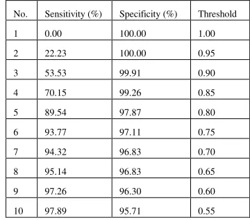
Results of Experiment Set 1.
Sensitivity and specificity under changing similarity threshold values on monochromic images (No number constraint for retrieved images)
No. Sensitivity (%) Specificity (%) Threshold
1 0.00 100.00 1.00
2 22.23 100.00 0.95
3 53.53 99.91 0.90
4 70.15 99.26 0.85
5 89.54 97.87 0.80
6 93.77 97.11 0.75
7 94.32 96.83 0.70
8 95.14 96.83 0.65
9 97.26 96.30 0.60
[image:5.612.331.511.502.660.2]10 97.89 95.71 0.55
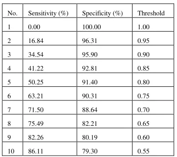
(b) Sensitivity and specificity under changing similarity threshold values on real life images (No number constraint for retrieved images)
Normally, we pay more attention to sensitivity than specificity due to sensitivity indicates the exploratory robustness (the ability to retrieve the truly similar images) of this retrieval system. However, specificity cannot be completely ignored, since there are cases where a system can achieve 100% sensitivity but 0% specificity. In this case, the system is still regarded to be of poor performance. The recommendable way is trying to achieve an as high sensitivity as possible without seriously compromising specificity. In this experiment set, we observe that, under a proper threshold value (0.80 for (a) and o.60 for (b)), CIRS can achieve a good sensitivity (89.54% for (a) and 82.26 for (b)) with still high specificity (97.87% for (a) and 80.19% for (b)).
Results of Experiment set 2.
Comparative evaluation on retrieval efficiency of naive one-by-one image matching approach and our approach
0 2 4 6 8 10 12 14 16
10
0
20
0
30
0
40
0
50
0
60
0
70
0
80
0
90
0
10
00
Line 1 Line 2
From Figure 1, we can clearly see that the execution time of one-by-one image matching is approximately 3 times as that of our image indexing approach. This experimental result reflects the better efficiency of our approach in compared with naive one-by-one image matching.
Note: Line 1 denotes the execution time line of one-by-one image matching, and line 2 denotes our image indexing approach. X-axis is the image No. (from 100 to 1000 images) and Y-axis is the execution time (measured in sec.).
6. CONCLUSIONS
In this paper, we have presented a color indexing scheme using two-level clustering processing for effective and efficient image retrieval. Two color feature summarizations, e.g. Local Color Centriods (LCCs) and Global Color Centroids (GCCs), are obtained by using two-level clustering processing and based on which a three-level R-tree is built to index database images. The experimental results on 1500 monochromatic images and 3000 real life images demonstrate the effectiveness and efficiency of this indexing scheme.
Currently, this image indexing is totally based on the color, which is the most important and useful factor in the image indexing and retrieval. Even so, we will still seek for the possibility of introducing the indexing mechanisms based on shape and texture, etc. This is believed to greatly enhance the potency of our system overall.
REFERENCES
[1] A. K. Jain. Data Clustering: A Review, ACM computing survey, vol.31, No.3, September 1999. [2] Eakins, J P and Graham, M E.: Content-based image
retrieval: a report to the JISC technology applications program, 1999.
[3] M. Swain and D. Ballard. Color Indexing. International Journal of Computer vision, 7(1): 11-32, 1991. [4] D. E. Knuth. Sorting and searching, the Art of
Computer Programming, vol.3. Reading, Mass.:Addison-Wesley, 1973.
[5] A.Guttman. R-trees: A dynamic index structure for spatial searching. In proceeding of the 1984 ACM SIGMOD Conference, pages 47-57, May 1984. [6] G. P. Babu, B. M. Mehtre, M. S. Kankanhalli. Color
indexing for efficient image retrieval. Multimedia Tools and Application, 1, 327-348, Kluwer Academic Publisher, Boston, 1995.
[7] E.C. Shek, A. Vellaikal, S. K. Dao, B. Perry. Semantic agents for content-based discovery in distributed image libraries, IEEE Workshop on Content-Based Access of Image and Video Libraries, Proceedings, pp 19-23, 1998. No. Sensitivity (%) Specificity (%) Threshold
1 0.00 100.00 1.00
2 16.84 96.31 0.95
3 34.54 95.90 0.90
4 41.22 92.81 0.85
5 50.25 91.40 0.80
6 63.21 90.31 0.75
7 71.50 88.64 0.70
8 75.49 82.21 0.65
9 82.26 80.19 0.60
10 86.11 79.30 0.55
[image:6.612.72.253.102.263.2]Figure 1. Comparison of execution time of one-by-one matching and our approach
[image:6.612.69.297.557.676.2]