Real-time dynamic substructuring in a coupled oscillator-pendulum system

White Rose Research Online URL for this paper:

http://eprints.whiterose.ac.uk/79695/

Version: Submitted Version

Article:

Kyrychko, Y.N., Blyuss, K.B., Gonzalez-Buelga, A. et al. (2 more authors) (2006) Real-time

dynamic substructuring in a coupled oscillator-pendulum system. Proceedings of the Royal

Society A, 462. 1271 - 1294. ISSN 1364-5021

https://doi.org/10.1098/rspa.2005.1624

[email protected] Reuse

Unless indicated otherwise, fulltext items are protected by copyright with all rights reserved. The copyright exception in section 29 of the Copyright, Designs and Patents Act 1988 allows the making of a single copy solely for the purpose of non-commercial research or private study within the limits of fair dealing. The publisher or other rights-holder may allow further reproduction and re-use of this version - refer to the White Rose Research Online record for this item. Where records identify the publisher as the copyright holder, users can verify any specific terms of use on the publisher’s website.

Takedown

If you consider content in White Rose Research Online to be in breach of UK law, please notify us by

coupled oscillator-pendulum system

By Y.N. Kyrychko1_{, K.B. Blyuss}2_{, A. Gonzalez-Buelga}3_,

S.J. Hogan1_{, D.J. Wagg}3

1_{Department of Engineering Mathematics, University of Bristol, Queen’s Building,}

Bristol BS8 1TR, UK

2_{Department of Mathematical Sciences, University of Exeter, Laver Building,}

Exeter EX4 4QE, UK

3_{Department of Mechanical Engineering, University of Bristol, Queen’s Building,}

Bristol BS8 1TR, UK

Real-time dynamic substructuring is a powerful testing method which brings together analytical, numerical and experimental tools for the study of complex structures. It consists of replacing one part of the structure with a numerical model, which is connected to the remainder of the physical structure (the substructure) by a transfer system. In order to provide reliable results, this hybrid system has to remain stable during the whole test. One of the problems with the method is the presence of delay (due to several technical factors) which can lead to destabilization and failure. In this paper we apply the dynamic substructuring technique to a simple nonlinear system, consisting of a pendulum attached to a mass-spring-damper. The latter is replaced by a numerical model and the transfer system is an actuator. The system dynamics is governed by two coupled second order neutral delay differential equations. We carry out a stability analysis of the system and identify possible regions of instability and the number of stability switches depending on parameters and the size of the delay. Using the parameters from a real experiment, we perform numerical simulations which confirm our analytical findings, and show regions of periodic and quasi-periodic behaviour. We also confirm our stability results by comparison with an experiment. The agreement is excellent.

Keywords: stability analysis; real-time testing; neutral delay equation; hopf bifurcation; numerical simulations

1. Introduction

experimental methods whilst at the same time avoiding their drawbacks. Such a hybrid testing method could help to reduce the overall cost of the experiment and at the same time offer the possibility of observing full scale dynamics.

One such approach is real-time dynamic substructuring (see, for instance, Blake-boroughet al.2001; Bonelli & Bursi 2004; Horiuchi & Konno 2001; Nakashima 2001; Pintoet al.2004; Wallaceet al2004; Williams & Blakeborough 2001). This method consists of dividing the test structure into two parts. One part is modelled numer-ically and the other is a physical substructure which is placed in the laboratory. The two parts are linked through a transfer system, usually sets of actuators. A significant concern is to ensure that the substructure and its numerical counterpart behave in the same way as the full structure. One of the main obstacles with this approach is the presence of delay.

Delay arises because of the non-instantaneous nature of the transfer system. In fact, there can be a number of different delays from several different sources, such as data acquisition, computation, digital signal processing and the actuator itself, which all contribute to produce an overall delay. In general, the dynamics of the transfer system (depending on its configuration) should be described by an inclusion of time delay and a frequency dependent delay (or time lag). However, the experiment presented in this paper has a transfer system represented by an electro-dynamic actuator, and we are working in the regime of small frequencies. This means that in this case the dependence of time delay on frequency of exter-nal excitation is negligible, and therefore, we treat time lag as a fixed time delay. This convention has been successfully used by several authors, including Darby

et al.(2001) and Darby et al.(2002). We have also produced the transfer system

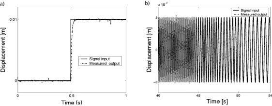
response plots 2 (a)), with the transfer function written via Laplace transform as

Y(s) = 56.02

s+ 55.55, and experimental frequency sweep testing is presented in Figure 2 (b)). Therefore the dynamics of the numerical part will be modelled using delay differential equations, or DDEs (partial or ordinary, depending on the complexity of the system). These equations depend not only on the current state of the system, but also on the history of the system over some previous time interval (the delay). Hence, the initial state space and the solution space of the delayed dynamical sys-tem are infinite dimensional. The theory of this type of equations lies in the area of functional differential equations discussed in details by Wu (1996), and some methods and results with applications to engineering problems can be found in Xu & Chung (2003).

00 00 11 11

00 00 00 00 00 00 00

11 11 11 11 11 11 11 00 00 11 11

F_ext M

C K Numerical model

Send measured forces to numerical model Transfer system

(actuator)

F measured

Physical substructure

b)

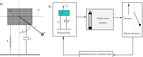
Figure 1. (a) Full coupled pendulum-MSD system. (b) Real-time dynamic substructuring system showing numerical model, transfer system and physical substructure.

coupled pendulum-MSD systems include the modelling of human leg motion (see, for example, Coveneyet al.2001; Lafortune & Lake 1995).

In order to investigate whether the hybrid system of substructure and numeri-cal model (figure 1(a)) behaves in the same way as the full structure would behave (figure 1(b)), we propose a model represented by delay differential equations. The whole system should remain stable during a test. However, delays can destabilize the system, giving rise to oscillatory, periodic or even chaotic solutions not present in the original non-delayed system. Therefore, a full mathematical analysis and numerical simulations based on experimental values of parameters will provide de-tailed information about the influence of delay on stability of the system. This will help to determine and then implement a delay compensation technique to be used in the experiment. The approach of using delay differential equations for mathe-matical modelling of hybrid testing has been first proposed by Wallaceet al.(2004) and Wallace et al.(2005). The authors considered a simple mass-spring oscillator and demonstrated the dependence of stability of the system on delay. Significant difference of the present work from earlier studies is the fact that we consider a nonlinear and neutral system of delay differential equations. For the general ref-erences on the theory of DDEs see, for example, Kuang (1993), Diekmannet al.

(1995), St´epan (1989) and references therein.

The paper is organized as follows: in Section 2 we introduce a system of delay differential equations describing the coupled pendulum-MSD system. Section 3 is devoted to the stability analysis of the neutral DDE. In Section 4 stability of peri-odic solutions is investigated by means of multiple scale analysis for the case of near resonant soft excitation. Section 5 contains numerical simulations which confirm our analytical findings. The linearized stability analysis of the coupled non-linear sys-tem of delay differential equations is presented in Section 6. Section 7 contains a comparison between experimental and analytical results. In Section 8 the effects of viscous damping are studied. The paper concludes with a summary of results in Section 9.

2. The equations of motion

Figure 2. (a) Transfer function step response. (b) Frequency sweep plot.

denoted by θ. We assume linear viscous damping C acting on the massM. The system is shown schematically in figure 1. The equations of motion for our system are

My¨(t) +Cy˙(t) +Ky(t) =Fext−my¨−mℓ[¨θsinθ+ ˙θ2cosθ],

mℓ2_{θ¨(t) +κθ˙(t) +mgℓsinθ(t) +mℓy¨sinθ(t) = 0,}

(2.1)

where

Fext=kcos(Ωt),

is the external excitation force applied in theydirection,CandKare the damping and stiffness coefficients respectively, and a dot indicates the derivative with respect to timet. We will refer toy(t), ˙y(t) and ¨y(t) as the position, velocity and acceleration of the MSD at timet. There are three important frequencies associated with this system: the natural frequency of the pendulumω0, where ω20 = g/ℓ, the natural frequency of the mass-spring-damperω1, whereω21=K/(M+m) and the frequency Ω of the external excitation force. The situation where the natural frequencies of the MSD and the pendulum are in 2 : 1 resonance has been widely studied in the literature (see Tondlet al.2000 and references therein).

Since the transfer system produces an unavoidable delay in the system, the feedback force will be delayed. The time delay is denoted byτ and it is assumed to be constant and non-negative. To account for the delay in the displacement signal, the force in the system (2.1) has to be described by the delayed state of the numerical model of the MSD. Therefore, in the RHS of the first equation in (2.1) we replacey(t) andθ(t) by their delayed counterparts:y(t−τ) andθ(t−τ) respectively. The same has to be done for allterms in the second equation of the system (2.1). By inserting these expressions in system (2.1), we obtain the following

My¨(t) +Cy˙(t) +Ky(t) +my¨(t−τ)

+mℓ[¨θ(t−τ) sinθ(t−τ) + ˙θ2_{(t−τ) cosθ(t−τ)] =kcos(Ωt),}

mℓ2_θ¨(t

−τ) +κθ˙(t−τ) +mgℓsinθ(t−τ) +mℓy¨(t−τ) sinθ(t−τ) = 0.

(2.2)

3. Stability analysis of the neutral delay differential equation

First, we consider the case when the angleθis small (θ≪1). In this case the system (2.2) decouples and we concentrate on the first equation, which describes the vertical motion of the pendulum-MSD system. In the absence of external forcing (k = 0), linearization of this equation around the trivial solution leads to the equation

My¨(t) +Cy˙(t) +Ky(t) +my¨(t−τ) = 0. (3.1)

Since the delayed system depends on the acceleration of the state variable, equation (3.1) is of a neutral type. We introduce the following non-dimensional variables:

ˆ

t=ω2t, τˆ=ω2τ, ω2=

r K M, p=

m M, ζ=

C

2√M K.

Under this rescaling and dropping the hats, equation (3.1) becomes

¨

z+ 2ζz˙+z+pz¨(t−τ) = 0, (3.2)

where dot means differentiation with respect to t. This equation has one trivial steady statez= ˙z= 0. The corresponding characteristic equation is

λ2_{+ 2ζλ+ 1 +pλ}2_e−λτ _{= 0. (3.3)}

Whenτ = 0, one obtains λ = −ζ±pζ2_{−1−p/(1 +p), so the steady state}

z= 0 is locally asymptotically stable. In the case|p|>1, this steady state is always unstable for any positive delay τ. (This already provides us with an important consideration when constructing the hybrid system, namely that for stability we must always haveM > m.) Therefore, we assume|p|<1 in all our further analysis. The purely imaginary eigenvalues occur whenλ=±i̟ for̟6= 0, so from (3.3)

−̟2+ 2iζ̟+ 1−p̟2e−i̟τ = 0.

Separating into the real and imaginary parts, we arrive at the following

−̟2_{+ 1}

−p̟2_{cos (̟τ) = 0,}

2ζ̟+p̟2sin (̟τ) = 0. (3.4) Upon squaring and adding these equations, we obtain

(1−p2_)̟4_{+ (4ζ}2

−2)̟2_{+ 1 = 0.} Solving for̟ gives

̟2

±=

1 (1−p2₎

h

(1−2ζ2₎

±p(1−2ζ2₎2_−(1−p2₎i_{. (3.5)} We observe that there can be either zero, one (repeated) or two real positive roots, depending on the values of p and ζ. This relation provides us with the explicit expressions for the stability boundaries, i.e. a family of solutions for the delay time

τ has the form

τ= 1

̟_±

Arctan 2ζ̟±

̟_±2₋₁ ±πn

, (3.6)

(p

(p

2,τ2) _(p 3,τ3 1

) ,τ

1)

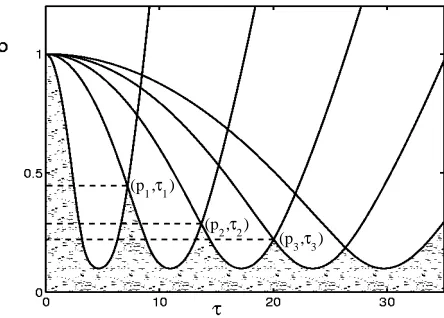
Figure 3. Stability of the trivial solution of the system (3.2) in the parameter space of

delay timeτ andpforζ <1/√2.

Lemma 3.1. _{The solution z= ˙z= 0of the system (3.2) is locally asymptotically}

stable forζ > 1

√

2 and|p|<1 independent of the delay time τ >0.

The proof of this lemma immediately follows from the expression (3.5) for̟_±. In terms of the original parameters, the conditions of lemma 3.1 state thatC2_{>2M K,}

M > m. These conditions perfectly justify the choice of pendulum as the physical substructure. In the physical system, if the damping is high enough, unconditional stability is guaranteed.

Next, consider the case ζ < 1/√2, which is depicted in figure 3. The shaded area shows the stability region. In this situation, stability of the trivial steady state strongly depends on the value of the delayτ. As τ increases from zero, the steady state undergoes a Hopf bifurcation, as a pair of complex conjugate roots of the characteristic equation crosses the imaginary axis. Under certain non-degeneracy conditions, this implies the birth of periodic solutions. We summarize our findings in the following lemma.

Lemma 3.2. _{Assume ζ < 1/}√_{2. The trivial solution of system (3.2) is locally}

asymptotically stable in the region

p <2ζp1−ζ2_{, (3.7)}

for all positive delay timesτ. In the region

2ζp1−ζ2_{≤p <1,}

the trivial solution is locally asymptotically stable for values of delay satisfying

0< τ < 1 ̟+

2π−Arccos1−̟

2 +

p̟2 +

1

̟₋

2πn−Arccos1−̟

2

−

p̟2

−

< τ < 1 ̟+

(2n+ 2)π−Arccos1−̟

2 +

p̟2 +

,

Proof. First we note that when the condition (3.7) holds, the square root

p

(1−2ζ2₎2_−(1−p2₎ in the definition of ̟2

± (3.5) is purely imaginary. Thus the eigenvalues of the

linearization matrix never cross the imaginary axis, and consequently, the trivial steady state is stable for all delay timesτ ≥0 in this region.

Next, we consider the situation when 2ζp1−ζ2 _{≤ p < 1. In this case the} characteristic polynomial (3.3) has two imaginary solutionsλ_± = i̟_± with̟+>

̟₋>0 defined in (3.5). In order to determine stability asτvaries, we need to find the sign of the derivative of Re(λ) at the points whereλ(τ) is purely imaginary. The technique we shall use has been widely applied to various characteristic equations (see, for example, Kuang 1993). Considering the functionλ=λ(τ) in equation (3.3) and differentiating this equation with respect toτ, one obtains

2λ+ 2ζ+pλ(2−λτ)e−λτdλ dτ =pλ

3

e−λτ.

From the last expression it follows that

_dλ

dτ −1

= 2(λ+ζ)e−

λτ_+pλ

pλ3 −

τ λ,

and from (3.3) we have

eλτ=− pλ

2

λ2_{+ 2ζλ+ 1}. Hence,

sgn

d(Reλ)

dτ

λ=i̟

= sgn

(

Re

dλ dτ

−1)

λ=i̟

= sgn{2ζ2

−1 +̟2₍₁

−p2₎

}.

Substituting̟2

± into the last expression, it is clear that the sign is positive for̟2+ and negative for̟2

−. This means that asτincreases and takes a value corresponding

to ̟+, λ crosses from the left to the right hand half of the complex plane. This implies the loss of stability of the trivial solution. Similarly, forτ corresponding to

̟₋, the crossing is from right to left, and stability is regained. The whole process is graphically illustrated in figure 3. The proof of the lemma is complete.

From lemma 3.2 it follows that as τ increases, the trivial equilibrium under-goes successive changes in its stability. However, it is worth noting that for fixed parameter values there is only afinitenumber of stability switches, and eventually this equilibrium becomes unstable. We can now find the number of these stability switches and the maximal delay beyond which the stability will never be recov-ered. The problem of constructing sequences of stability switches was addressed for first-order neutral equations by Wei and Ruan (2002).

Let us introduce a sequence

wherepn, n= 1, ...solve the equation

τ₋(n) =τ+(n+ 1). (3.8) Here we have used the notation

τ+(n) = 1

̟+

2πn−Arccos 2ζ̟+

̟+2−1

, τ₋(n) = 1

̟₋

2πn−Arccos 2ζ̟−

̟₋2₋₁

.

Theorem 3.3. _{If p1 ≤ p < 1 there is one stability switch at τ+(0). The trivial}

equilibrium is stable for0≤τ≤τ+(0)and unstable forτ > τ+(0). Ifpk+1≤p < pk

for k = 1, ..., then there are exactly (2k+ 1) stability switches, and the trivial equilibrium is stable for

(0, τ+(0))∪(τ−(1), τ+(1))∪...∪(τ−(k), τ+(k)),

and unstable for

(τ+(0), τ₋(1))∪(τ+(1), τ₋(2))∪...∪(τ+(k),∞).

For a given value ofp, theorem 3.3 gives the regions of linear stability in terms of delay timeτ. Unlesspis smaller than the lower stability boundarypc = 2ζ

p

1−ζ2_, there always exists a sufficiently large delayτ after which the system will be un-stable. The stable boundaries of the origin can be located by the branchesτ+ and

τ₋ which satisfy τ+(n)> τ₋(n) forn= 1,2, .... For example, whenτ crossesτ₋(1) the unstable origin becomes stable. Whenτ is increased further to crossτ+(1), the stability is lost again as a pair of eigenvalues cross the imaginary axis into the right half plane. Similarly, other stability regions can be found forτ₋(n)< τ < τ+(n). Each time we cross the stability boundary into an unstable region, the delayed action of the pendulum on the MSD leads to a destabilization of numerical model. In the points (p, τ) = (pn, τn) the system undergoes a codimension-two Hopf

bifurcation. There is a pair of complex conjugate eigenvalues crossing the imaginary axis from left to right, and there is another pair crossing from right to left. Therefore, at the above points, the system has two frequencies simultaneously present. Possible resonances in this case were studied by Campbell (1997).

4. Hopf Bifurcation

In this section the Hopf bifurcation will be investigated. Linearizing equation (2.2) withk6= 0, and rescaling using ˆk=k/K and ˆΩ = Ω/ω2, we obtain, after dropping the hats:

¨

z+ 2ζz˙+z+pz¨(t−τ) =kcos Ωt. (4.1)

which is simply equation (3.2) with the forcing included. In order to study the criticality of the bifurcation, we will resort to a multiple scales method. Taking a delay timeτ =τc+ετ1, whereτc is the critical delay time, we letT =εt be the

embarking on series expansion analysis, it is worth noting that since we are crossing the stability boundary, the following relation holds:

p= 1

̟2

±

q

(̟2

±−1)2+ 4ζ2̟±2.

Looking for solutions of equation (4.1) in the form

z(t) =z0(t, T) +εz1(t, T) +. . . , we obtain at orderO(1)

∂2

∂t2z0+ 2ζ

∂

∂tz0+z0+pΩ ∂2

∂t2z0(t−τc, T) = 0, wherepΩ=

p

(Ω2₋₁₎2_{+ 4ζ}2_Ω2_/Ω2_{. The solution of this equation is}

z0(t, T) =A(T)eiΩt+A∗(T)e−iΩt, (4.2) whereA(T) is an as yet undetermined amplitude of oscillation. At orderO(ε1_{) we} have

∂2

∂t2z1+2ζ

∂

∂tz1+z1+pΩ ∂2

∂t2z1(t−τc, T) =−2

∂ ∂t

∂ ∂Tz0−2ζ

∂

∂Tz0−2pΩ ∂ ∂t

∂

∂Tz0(t−τc, T)

−pΩτ1

∂3

∂t3z0(t−τc, T) +σpˆΩ

∂2

∂t2z0(t−τc, T) +kcos Ωt, (4.3) with ˆpΩ= 2(Ω2−1−4ζ2)/(Ω3

p

(Ω2₋₁₎2_{+ 4ζ}2_{). Substitutingz}

0from (4.2) in the last expression and using complex notation, gives

∂2

∂t2z1+ 2ζ

∂

∂tz1+z1+pΩ ∂2

∂t2z1(t−τc, T) =

−2iΩAT −2ζAT −2ipΩΩe−iΩτcAT + iτ1pΩΩ3A−σpˆΩΩ2A+

k

2

eiΩt+ c.c.,

whereAT =∂A/∂T andc.c.denotes the complex conjugate. To avoid secular terms

we set the bracket on the right hand side equal to zero. This gives us an equation for the amplitudeAin the form:

−2AT(iΩ +ζ+ ipΩΩe−iΩτc) = (σpˆΩ−ipΩτ1Ω)Ω2A−

k

2. (4.4)

This equation can be transformed into

AT = 1

2

τ1pΩΩ2+σpˆΩΩ2ζ

ζ2_{+ 1/Ω}2 + i

σpˆΩΩ−pΩτ1ζΩ3

ζ2_{+ 1/Ω}2

A−k_4ζ2ζ_{+ 1}+ i/_/Ω_Ω2. WritingA=u+ivand separating real and imaginary parts, we obtain the following linear system of differential equations:

uT =αu−βv+c1,

where we have introduced the notation

α=1 2Ω

2τ1pΩ+σpˆΩζ

ζ2_{+ 1/Ω}2 , β= 1 2Ω

σpˆΩ−pΩτ1ζΩ2

ζ2_{+ 1/Ω}2 ,

c1=−

k

4

ζ

ζ2_{+ 1/Ω}2, c2=−

k

4

1 Ω(ζ2_{+ 1/Ω}2₎. System (4.5) can be solved to yield

u(T) = 1 2

σpˆΩk Ω2_(σ2_pˆ2

Ω+p 2 ΩΩ2τ

2 1)

+C1eαTcosβT+C2eαTsinβT,

v(T) = 1 2

pΩkτ1 Ω (σ2_pˆ2

Ω+p 2 ΩΩ2τ

2 1)

−C2eαTcosβT+C1eαTsinβT.

(4.6)

Thus, one can observe that the amplitudeAT of the bifurcating periodic solution

is proportional to the amplitudekof the forcing, and is also modulated on a longer time scale as shown by the above expressions. Ifk= 0 (and consequently σ= 0), then depending on the sign ofτ1, the u(T) and v(T) exponentially tend to either 0 or±∞, thus indicating that the periodic solution is unstable. However, ifk6= 0, then there is a periodic solution

z(t) = σpˆΩk Ω2_(σ2_pˆ2

Ω+p2ΩΩ2τ12)

cos(Ωt+θ0) +O(ǫ), which is stable if

τ1pΩ+σpˆΩζ <0, (4.7)

and unstable otherwise.

5. Numerical simulations

In this section we perform a numerical simulation of the system (4.1). The equation was discretized using an explicit finite difference scheme. The damping term was approximated by central differences to improve numerical stability.

For all simulations we set p= 0.2. In terms of the original parameters of the system this means that the mass of the pendulum is five times smaller than the mass of the MSD. At the same time, the scaled damping coefficientζis taken to be

ζ= 0.05. It readily follows thatp >2ζp1−ζ2_{, and one can expect a succession of} stability switches for increasing values ofτ.

The numerical timestep for the simulations is kept at ∆t = 0.01. To illustrate the behaviour of solutions in stable and unstable regions, as discussed in section 3, we will move along theτ-axis and observe changes which occur as the stability boundaries are crossed.

0 50 100 150 −1

−0.8 −0.6 −0.4 −0.2 0 0.2 0.4 0.6 0.8 1

t z(t)

0 50 100 150 200

−400 −300 −200 −100 0 100 200 300 400

t z(t)

0 50 100 150

−1 −0.8 −0.6 −0.4 −0.2 0 0.2 0.4 0.6 0.8 1

t z(t)

0 50 100 150 200

−100 −80 −60 −40 −20 0 20 40 60 80

t z(t)

a) b)

c) d)

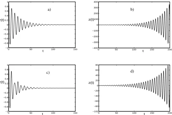
Figure 4. Temporal dynamics ofz(t) of system (3.2) for (a)τ= 1, (b)τ = 5, (c)τ = 7.5

and (d)τ= 11.

solution remains asymptotically stable and quickly decays to the trivial steady state (figure 4(a)). Since oscillatory decay is observed, this indicates that the eigenvalues of characteristic equation have non-zero imaginary part. Figure 4(b) shows the sit-uation when the first switch from stability to instability has occurred (τ= 5). The characteristic eigenvalues have crossed the imaginary axis, and hence the trivial state has become unstable. Stability is regained in figure 4(c) forτ= 7.5. It can be observed in this picture that there exist different frequencies of oscillations. When

τ is larger still, stability is lost again (figure 4(d),τ= 11).

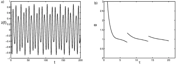
As the system recovers its stability as shown in figure 5(a), one can clearly see the appearance ofbeats. Even though the eigenvalues of the characteristic equation still have negative real part (as can be seen in the way the oscillations decay), it now takes a much longer time for the system to eventually settle onto the trivial equilibrium. Figures 5(b) and 5(d) bear a close resemblance to earlier pictures illustrating the dynamics of the substructure in the unstable regime. Figure 5(c) indicates the beats increase in their amplitude while the decay slows down.

It is interesting to see the behaviour when the curves in figure 3 cross each other. These points correspond to the case when relation (3.8) holds. Forζ= 0.05, the first point p1 can be found at (p1, τ1) ≈ (0.4453,7.1859). As expected, the system undergoes a codimension-two Hopf bifurcation and exhibits quasi-periodic oscillations as shown in figure 5(a). Finally, figure 5(b) shows the dependence of the Hopf frequency on the delay timeτ. At the points of discontinuity, there are two frequencies of oscillations.

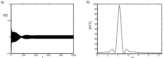
Next, the case when the external force is present (k 6= 0) will be studied. In figure 7 we show the solutionz(t) together with its Fourier spectrum for delay time

0 100 200 300 −1

−0.8 −0.6 −0.4 −0.2 0 0.2 0.4 0.6 0.8 1

t z(t)

0 50 100 150 200

−30 −20 −10 0 10 20 30

t z(t)

0 200 400 600

−1 −0.8 −0.6 −0.4 −0.2 0 0.2 0.4 0.6 0.8 1

t z(t)

0 50 100 150 200

−15 −10 −5 0 5 10 15

t z(t)

a) b)

c) d)

Figure 5. Temporal dynamics of system (3.2) for (a)τ= 14, (b)τ = 17, (c)τ = 20 and

(d)τ = 23.

Figure 6. (a) Solutionz(t) at the codimension-two point (p1, τ1)≈(0.4453,7.1859). (b)

Hopf frequency as a function of delay timeτ.

onto a stable limit cycle. The Fourier spectrum shown in figure 7 clearly possesses a sharp peak confirming periodic behaviour of the solution. The numerical value of the corresponding oscillation frequency, as found from the Fourier spectrum is

0 200 400 600 800 1000 −0.5

0 0.5 1

t z(t)

a)

0 1 2 3 4 5 6

0 10 20 30 40 50 60 70 80 90 100

ω

|FFT|

b)

Figure 7. (a) Solutionz(t) withτ= 1.55,k= 0.01, Ω = 2.1,p= 0.75166. (b) Fourier

spectrum of the solution.

6. Stability analysis of the full system

Now, we return to system (2.2), and rewrite it (without loss of generality) by omitting the delay in the second equation and settingFext= 0 to obtain

My¨(t) +Cy˙(t) +Ky(t) +my¨(t−τ)

+mℓ[¨θ(t−τ) sinθ(t−τ) + ˙θ2_(t

−τ) cosθ(t−τ)] = 0,

mℓ2_θ¨_{(t) +kθ}˙_{(t) +mgℓsinθ(t) +mℓy¨(t) sinθ(t) = 0.}

(6.1)

It is more convenient to rewrite these equations as a first order system. In order to do so, we introduce the new variables

x_{= (x1, x2, x3, x4)}T _{= (y, θ,y,˙ θ}˙₎T_.

With these variables, system (6.1) becomes

˙

x1 = x3, ˙

x2 = x4, ˙

x3 = −

1

M "

Cx3+Kx1+mx˙3(t−τ)

+mℓ

˙

x4(t−τ) sinx2(t−τ) +x24(t−τ) cosx2(t−τ)

#

,

˙

x4 = −

k mℓ2x4+

1

ℓM sinx2[Cx3−M g+Kx1+ ˙x3(t−τ)]

+m

M sinx2

˙

x4(t−τ) sinx2(t−τ) +x42(t−τ) cosx2(t−τ). (6.2)

The equilibria for this system are x _{= (0,0,0,0) and} x

n = (0, nπ,0,0), n =

1,2, .... Linearization near the trivial steady statex₌0_gives

˙

0 200 400 600 800 1000 −0.5 0 0.5 1 t z(t) a)

0 0.5 1 1.5 2 2.5 3

0 0.2 0.4 0.6 0.8 1 1.2 1.4 1.6 1.8 2x 10

4

ω

|FFT|

b)

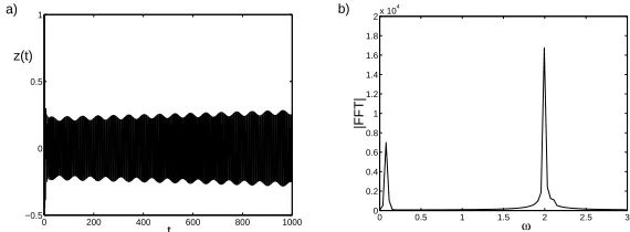
Figure 8. (a) Solutionz(t) withτ = 1.608,k= 0.01, Ω = 2.1,p= 0.75166. (b) Fourier

spectrum of the solution.

where matricesAandB are given by

A=             

0 0 1 0

0 0 0 1

−_MK 0 −_MC 0

0 −g_ℓ 0 −_mℓk2

            

, B=

          

0 0 0 0

0 0 0 0

0 0 −_Mm 0

0 0 0 0

           .

The characteristic polynomial becomes

λ2_+λ k

mℓ2+

g ℓ

λ2_{M +λC+K+λ}2_e−λτ_m

= 0. (6.3)

It is clear that stability is determined by the roots of the second multiplier in equation (6.3).

Similarly, for the steady statex

n= (0, nπ,0,0) the matricesAandB are given

by A=             

0 0 1 0

0 0 0 1

−_MK 0 −_MC 0

0 (−1)n+1g

ℓ 0 −

k mℓ2             

, B=

          

0 0 0 0

0 0 0 0

0 0 −m

M 0

0 0 0 0

           .

The corresponding characteristic polynomial is now

λ2_+λ k

mℓ2 + (−1)

ng

ℓ

λ2_M+λC+K+λ2_e−λτ_m

= 0. (6.4)

Table 1.Substructure and pendulum parameters

M[kg] C[kg/s] K[N/m] m[kg]

4 20 5000 0.9

such steady states are always unstable for any value of delayτ, includingτ= 0. For the case ofn even, the roots are determined by the same equation as in the case

n= 0 considered above. The second bracket in equations (6.3) and (6.4) is exactly equation (3.3) divided byM in its dimensional form.

7. Experimental results

In the previous sections we studied the stability of the model using analytical and numerical tools. In order to confirm our findings we need to perform some exper-imental tests, using the real time dynamic substructuring technique. As discussed in the Introduction, the pendulum is the physical substructure, the MSD is mod-elled numerically in the computer. The numerical model is used to calculate the displacement at the interface due to some external excitation. The displacement is applied to the substructure (pendulum) in real-time using an electro-mechanical actuator (the transfer system). The force acting on the physical substructure is measured via a load cell and fed back to the numerical model. This feedback force is used to calculate the displacement at the interface for the next time step. This process is repeated until the end of the test. To implement real-time tasks a dSpace DS1104 RD Controller Board is used; MATLAB/Simulink is employed to build the numerical model. The dSpace module ControlDesk is used for online analysis and control. The transfer system is an electrically driven ball-screw actuator with an in-line mounted synchronous servo-motor controlled by a servo-drive which applies a displacement to the pendulum pivot point in the vertical direction. The values of the system parameters are given in Table 1. It is worth noting that, since the MSD is represented by a numerical model,M,K andC can be changed easily from one test to another to observe different situations.

The first issue to be addressed in order to be able to develop successful sub-structuring tests is to ensure numerical model stability. We define stable as bounded input bounded output (BIBO) stable. In this case the output (displacement) will remain bounded for all time, for any initial condition and input. The numerical model in this case is always BIBO stable.

During the experiment the instability due to delay appears as a new frequency in the numerical model displacement, when the stability boundary is crossed. We start with a delay of 0.018s(the natural delay time of the transfer system) and the delay will be increased by 0.001s increments until the system becomes unstable, and the new frequency appears. The delay time is increased by holding the signals going to the actuator.

Figure 9. Stability charts showing the stability boundary with the parameters from Table 1: (a) theoretical chart and (b) experimental paths.

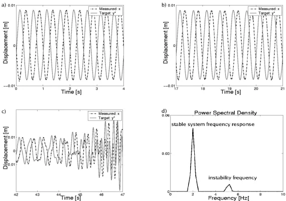
Figure 10. Changes in stability of the system while following path 1 shown in figure 9(b).

Numerical model is stable: (a) τ = 0.018s, (b) τ = 0.075s. (c) Instability frequency

appears,τ= 0.093s. (d) Fourier spectrum of the response: instability frequency 6.3Hz.

very small delay time τ. Then we follow path 1 (figure 9(b))until the stability boundary is reached. Once the boundary is crossed, the response of the system grows exponentially making it impossible to continue experimental testing (the actuator cannot achieve the required displacements). Consequently, it is technically impossible to increase the delay further in order to reach the stability area. In order to find the stability boundaries we start with the value of delay timeτ inside the next stability region. Decreasing or increasing the delay time, i.e. following path 2 and path 3 in figure 9(b) until the instability frequency appears. In this way the experimental values of stability switchesτ2 andτ3 will be found.

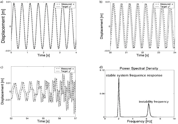
Figure 10 shows experimental records while following path 1. In figure 10(a) the measured solution x is plotted against its counterpart y∗ _{as determined by}

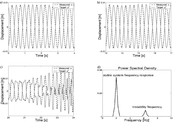
Figure 11. Changes in stability of the system while following path 2 shown in figure 9(b).

Numerical model is stable: (a)τ = 0.22s, (b)τ= 0.18s. (c) Instability frequency appears,

τ= 0.162s. (d) Fourier spectrum of the response: instability frequency 5.2Hz.

The experimental eigentriple at the first stability boundary is therefore (p, τ, ω) = (0.225,0.093,6.3).

Figure 11 illustrates the recorded signals when following path 2, when the delay is decreasing. The numerical model is stable until the delayτ reaches 0.162s, figure 11(c). The corresponding value of the instability frequency isω= 5.2Hz, as shown in figure 11(d). Hence, the experimental eigentriple for this crossing of stability boundary is (p, τ, ω) = (0.225,0.162,5.2).

The experimental results when following path 3 are depicted in figure 12. Now the numerical model remains stable until the delay timeτ reaches 0.255s, and the solution becomes unstable, figure 12(c). In this case, the instability frequency is

ω = 6.25Hz, as can be found from the Fourier transform of the solution at this point, as shown in figure 12(d). Therefore, this last boundary point in our analysis is characterized by the experimental eigentriple (p, τ, ω) = (0.225,0.255,6.25).

Figure 13 shows an excellent agreement between theoretical model and experi-mental results for stability boundaries. When the stability boundary is crossed, the solution very quickly becomes unstable and develops higher amplitude oscillations and irregular motions. This makes finding experimental values for stability bound-ary an extremely sensitive problem. This explains slight deviation of experimental values from the analytical prediction as illustrated in figure 13 a). In figure 13 b) we show experimental stability border points corresponding to different values of

p.

Figure 12. Changes in stability of the system while following path 2 shown in figure 9(b).

Numerical model is stable: (a) τ = 0.235s, (b) τ = 0.245s. (c) Instability frequency

appears,τ= 0.255s. (d) Fourier spectrum of the response: instability frequency 6.25Hz.

Table 2.Theoretical versus experimental instability frequencies, [Hz]

Instability frequency ωa ωb ωc

Experimental 6.3 5.2 6.25

Theoretical 6.2310 5.2139 6.2310

8. Viscous damping

In this section we consider the effect of velocity feedback on the dynamics of the pendulum-MSD system. This type of feedback becomes important when one takes into account the fact that the pendulum experiences the action of viscous damping. In this case, the vertical equation of motion for the numerical model in the absence of forcing takes the form

My¨+C1y˙(t) +Ky(t) +my¨(t−τ) +C2y˙(t−τ) = 0, (8.1) where C1 is the damping of the numerical model, and C2 is the viscous damping of the pendulum. Using the same scaling as in Section 3 and introducing the new variables

ζ1=

C1

2√M K, ζ2= C2 2√M K,

equation (8.1) transforms into

¨

z+ 2ζ1z˙+z+pz¨(t−τ) + 2ζ2z˙(t−τ) = 0. (8.2) The characteristic equation is now

λ2_{+ 2ζ}

Figure 13. (a) Comparison of experimental results with analytical predictions. (b) Experimental versus theoretical stability border.

τ p

a)

1

0.8

0.6

0.4

0.2

0 2 4 6 8

ζ1=0.05,ζ2=0

ζ1=0.05,ζ2=0.025

ζ1=0.05,ζ2=0.045

ζ1=0.05,ζ2=0.05

τ p

4

2 6 8

1

0.8

0.6

0.4

0.2

0 b)

ζ1=0.05,

stable region

unstable region

stable region =0.125

2 ζ

Figure 14. (a) Critical stability boundaries for different values of viscous damping. (b) Disjoint stability boundary for a large value of viscous damping.

Transition to instability occurs whenλ=±i̟, ̟ >0. Substituting this into the characteristic equation and separating real and imaginary parts gives the following system

−̟2_{+ 1}

−p̟2_{cos̟τ+ 2ζ}

2̟sin̟τ = 0, 2ζ1+p̟sin̟τ + 2ζ2cos̟τ = 0.

(8.4)

Squaring and adding these two equations, we obtain an equation for̟, which can be solved to give

̟2

±=

1 (1−p2₎

(1 + 2ζ2

2−2ζ12)±

q

(1 + 2ζ2

2−2ζ12)−(1−p2)

. (8.5)

Employing the same methods as the ones used in Section 3, one can prove the fol-lowing theorem concerning the stability of the trivial solution.

Lemma 8.1. _{Let 1 + 2ζ}2

2 −2ζ12 < 0. Then for |p| < 1 the trivial solution is

asymptotically stable for any delay timeτ >0. If, however, 1 + 2ζ2

2−2ζ12>0, then

the trivial solution of system (3.2) is locally asymptotically stable in the region

p <2

q

(1−ζ2

1−ζ22)(ζ12−ζ22), (8.6)

for all positive delay timesτ. In the region

2

q

(1−ζ2

the trivial solution is locally asymptotically stable for values of delay satisfying

0< τ < 1 ̟+

2π−Arccosp(1−̟

2

+)−4ζ1ζ2

p2_̟2 ++ 4ζ22

1

̟₋

2πn−Arccosp(1−̟

2

−)−4ζ1ζ2

p2_̟2

−+ 4ζ22

< τ < 1 ̟+

(2n+ 2)π−Arccosp(1−̟

2

+)−4ζ1ζ2

p2_̟2 ++ 4ζ22

,

wheren= 1,2, ....

It is worth noting that in the limitζ2→0 the results of this lemma coincide with those of lemma 3.2. Furthermore, as it is clear from relation (3.7), these stability results are only valid if one imposes an additional but experimentally reasonable requirement ζ2 < ζ1. Physically this means that the viscous damping C2 of the pendulum is smaller than that of the mass-spring-damper.

We illustrate in figure 14(a) the changes to the stability boundary as the viscous damping is increased from 0 until it reaches the value of the damping of MSD. As the viscosity increases, the stability area gets smaller and stability boundary shifts to the left. Eventually, as can be seen in figure 14(b), after touching zero the stability boundary disintegrates and splits into separate stability regions. As any vibration will eventually die down in these regions, they are calledamplitude death

regions or death islands(see, for instance, Xu & Chung 2003). These regions are experimentally important for controlling the stability of the system. Experimental results regarding the stability of the system with viscous damping can be found in Gonzalez-Buelgaet al. (2005).

We can explain figure 14 physically. The critical stability boundary first touches theτ axis (p= 0) when ζ1 =ζ2 andτ =π. From equation (8.2) we can see that this corresponds to the case when the contribution to the damping, through the term 2ζ1z˙, is exactly balanced by an equal (ζ1 =ζ2) and opposite (out of phase, sinceτ =π) contribution, through the term 2ζ2z˙(t−τ). In this case ̟_±= 1 and the resulting solution is neutrally stable since λ=±i. Asζ2 then increases, there is a finite range of τ for p = 0 when the delayed damping due to the pendulum exceeds that due to the numerical model. In that range the trivial solution is then unstable.

9. Conclusions

In this paper the real-time dynamic substructuring technique has been investigated for the system consisting of a mass-spring-damper and a pendulum attached to it. We introduced a system of two second order delay differential equations, with one of them being neutral. This approach of modelling allows us to account for the delay which naturally arises during the test.

that there is a finite number of them for fixed system parameters and proposed a scheme for calculating their number. After the presence of a Hopf bifurcation had been established, the stability of the bifurcating periodic solutions was studied using the method of multiple scales. This has also provided analytical expressions for the amplitude and frequency of the periodic orbit, together with an easily verifiable condition for stability.

The numerical simulations which are presented in Section 5 confirm our theo-retical findings, and convergence to the steady state can be observed in the stable regions while blow-up of solutions in finite time is shown in the unstable regions. Moreover, quasi-periodic oscillation of the solution is also illustrated and the exis-tence of thebeatsis detected. The Hopf frequency as a function of the delay time shows the presence of two frequencies of oscillation at the codimension-two Hopf bifurcation points. In the case of non-zero forcing our numerical results illustrate two possibilities: the solutions asymptotically approach a stable limit cycle or they are modulated on a long time scale by a growing harmonic. In Section 6 we return to the original system and study its linearized stability.

In order to confirm the validity of our analytical considerations, we performed a series of experimental tests. The stability boundary of the trivial solution was in good agreement with analytical prediction, as were the instability frequencies. The stability of the solution was explored for different values of the delay time τ, and the appearance of instability frequency detected in each case.

We have also considered the case of viscous damping present in the system. This has its effect on the stability boundary as it distorts and shrinks in size. For very large damping the stability area transforms into disjoint death islands separated by instability regions.

Overall, the study in this paper is a first step of modelling nonlinear and more complex substructures using DDEs. Future plans include the modelling of large scale engineering structures, such as suspension bridge cables, and mechanical systems, including the damper units for helicopter rotors.

The authors would like to acknowledge the support of the EPSRC: YK is supported by EPSRC grant (GR/72020/01), KB is supported by EPSRC grant (GR/S31662/01), AGB is supported by EPSRC grant (GR/S49780) and DJW via an Advanced Research

Fellowship. SJH is grateful to Centre de Recerca Matem`atica, Bellaterra, Catalunya for

providing facilities to complete part of this project.

References

Blakeborough, A., Williams, M.S., Darby, A.P. & Williams, D.M. 2001 The development

of real-time substructure testing.Phil. Trans. R. Soc.A359_{, 1869 - 1891.}

Bonelli, A. & Bursi, O.S. 2004 Generalized-a methods for seismic structural testing.

Earthq. Eng. Struct. Dyn.33_{, 1067-1102.}

Campbell, S.A. 1997 Resonant codimension two bifurcation in a neutral functional

differ-ential equation.Nonl. Anal. TMA30_{, 4577-4594.}

Coveney, V.A., Hunter, G.D. & Spriggs, J. 2001 Is the behaviour of the leg during

oscil-lation linear?J. Biomech.34, 827-830.

Darby, A.P., Blakeborough, A. & Williams, M.S. 2001 Improved control algorithm for

real-time substructure testing.Earthq. Eng. Struct. Dyn.30_{, 431-448.}

Darby, A.P., Williams, M.S. & Blakeborough, A. 2002 Stability and Delay Compensation

Diekmann, O., van Gils, S., Verduyn Lunel, S.M. & Walther, H.-O. 1995Delay Equations: Functional, Complex, and Nonlinear Analysis, vol. 110, Springer-Verlag, New York. Gonzalez-Buelga,A., Wagg, D.J. & Neil S.A. 2005 A hybrid numerical-experimental model

of a coupled pendulum-mass-spring-damper system. submitted toInt. J. Nonl. Mech..

Horiuchi, T., Konno, T. 2001 A new method for compensating actuator delay in real-time

hybrid experiments.Phil. Trans. R. Soc.A359_{, 1893 - 1909.}

Hu, H.Y. & Wang, Z.H. 2002 Dynamics of controlled mechanical systems with delayed

feedback. Springer-Verlag, New York.

Kuang, Y. 1993 Delay differential equations with applications in population dynamics.

Academic Press, San Diego.

Lafortune, M.A. & Lake, M.J. 1995 Human pendulum approach to simulate and quantify

locomotor impact loading.J. Biomech.28_{, 1111-1114.}

Nakashima, M. 2001 Development, potential, and limitations of real-time online (pseudo

dynamic) testing.Phil. Trans. R. Soc.A359 , 1851-1867.

Pinto, A.V., Pegon, P., Magonette,G. & Tsionis, G.2004 Pseudo-dynamic testing of bridges

using non-linear substructuring.Earthq. Eng. Struct. Dyn.33_{, 1125-1146.}

St´epan, G. 1989Retarded dynamical systems: stability and characteristic functions.

Long-man, London.

Tondl, A., Ruijgrok, T., Verhulst, F. & R. Nabergoj 2000 Autoparametric resonance in

mechanical systems. CUP, Cambridge.

Wallace, M.I., Sieber, J., Neild, S.A., Wagg, D.J. & Krauskopf, B. 2005 Delay differen-tial equation models for real-time dynamic substructuring. Accepted for publication in

Earthq. Eng. Struct. Dyn..

Wallace, M.I., Neild, S.A. & Wagg, D.J. 2004 An adaptive polynomial based forward prediction algorithm for multi-actuator real-time dynamic substructuring. Submitted toProc. R. Soc. Lond.A.

Wei, J.J. & Ruan, S. 2002 Stability and global Hopf bifurcation for neutral differential

equations.Acta. Math. Sinica45_{, 93-104.}

Williams, M.S. & Blakeborough, A. 2001 Laboratory testing of structures under dynamic

loads: an introductory review.Phil. Trans. R. Soc.A359_{, 1651 - 1669.}

Wu, J. 1996 Theory and Applications of Partial Functional Differential Equations.

Springer-Verlag, New York, 1996.

Xu, J. & Chung, K.W. 2003 Effects of time delayed position feedback on a van der