Meta heuristic algorithms for optimized network flow wavelet based image coding

warwick.ac.uk/lib-publications

Original citation:

Kusetoğulları, Hüseyin, Leeson, Mark S., Kole, Burak and Hines, Evor. (2014) Meta-heuristic

algorithms for optimized network flow wavelet-based image coding. Applied Soft

Computing, 14 (Part C). pp. 536-553.

Permanent WRAP URL:

http://wrap.warwick.ac.uk/58843

Copyright and reuse:

The Warwick Research Archive Portal (WRAP) makes this work by researchers of the

University of Warwick available open access under the following conditions. Copyright ©

and all moral rights to the version of the paper presented here belong to the individual

author(s) and/or other copyright owners. To the extent reasonable and practicable the

material made available in WRAP has been checked for eligibility before being made

available.

Copies of full items can be used for personal research or study, educational, or not-for-profit

purposes without prior permission or charge. Provided that the authors, title and full

bibliographic details are credited, a hyperlink and/or URL is given for the original metadata

page and the content is not changed in any way.

Publisher’s statement:

© 2017, Elsevier. Licensed under the Creative Commons

Attribution-NonCommercial-NoDerivatives 4.0 International

http://creativecommons.org/licenses/by-nc-nd/4.0/

A note on versions:

The version presented here may differ from the published version or, version of record, if

you wish to cite this item you are advised to consult the publisher’s version. Please see the

‘permanent WRAP url’ above for details on accessing the published version and note that

access may require a subscription.

BR`N

-

URa^V_`VP 7YT\^V`UZ_ S\^ D]`VZVfRQ CR`c\^X

=Y\c KNbRYR`

-

ON_RQ @ZNTR 9\QV[T

Huseyin Kusetogullari1,*, Mark S. Leeson2, Burak Kole2and Evor L. Hines2

1_{Department of Computer Engineering, Gediz University, Izmir, Turkey} 2

School of Engineering, University of Warwick, Coventry, CV4 7AL, UK

Abstract: Optimal multipath selection to maximize the received multiple description coding (MDCs) in a lossy

network model is proposed. Multiple Description Scalar Quantization (MDSQ) has been applied to the wavelet

coefficients of a color image to generate the MDCs which are combating transmission loss over lossy networks. In

the networks, each received description raises the reconstruction quality of an MDC-coded signal (image, audio or

video). In terms of maximizing the received descriptions, a greater number of optimal routings between source and

destination must be obtained. The Rainbow Network Flow (RNF) collaborated with effective meta-heuristic

algorithms is a good approach to resolve it. Two meta-heuristic algorithms which are Genetic Algorithm (GA) and

Particle Swarm Optimization (PSO) have been utilized to solve the multi-objective optimization routing problem for

finding optimal routings each of which is assigned as a distinct color by RNF to maximize the coded descriptions in

a network model. By employing a local search based priority encoding method, each individual in GA and particle

in PSO is represented as a potential solution. The proposed algorithms are compared with the multipath Dijkstra

algorithm

(MDA)

simulations run over various random network topologies and the results show that the PSO algorithm finds optimal

routings effectively and maximizes the received MDCs with assistance of RNF, leading to reduce packet loss and

increase throughput.

Keywords: Genetic algorithm (GA), particle swarm optimization (PSO), rainbow network flow (RNF),

multi-objective multipath optimization, routing representation, multiple description image coding, image transmission.

1. Introduction

The transmission of multimedia information over communication channels/paths has become a challenging problem

with the increased usage of multimedia services in networks. Transmitting original source (information) naturally

requires a significant amount of bandwidth and storage. This has been a strong motivation to examine and develop

an efficient optimization method in order to use less bandwidth as well as finding the optimum network routings.

In multimedia transmission, original source image should be compressed for reducing redundancy in the image as

well as efficient usage of bandwidth. There are two different approaches that have been applied to compress source

image [1]. The first is lossless, where a compact representation of the source coding can be decoded to reconstruct

#

Corresponding Author Tel.: +905423599211 E-mail address: [email protected]

*Manuscript

the original signal without error. The second is lossy, which causes distortion in the original signal and the exact

reconstruction of the original source cannot be achieved [1]. The purpose of using both techniques is to encode the

source into a compressed digital representation that can be used for transmission. However, packet transmission

problems such as packet dropping or congestion may occur over lossy transmission networks. For instance, there

may be encounters with low capacity links, network congestion or excessive delay to deliver packets. To combat

multimedia packet loss transmission problem, multiple description coding (MD coding or MDC) transmitting

through multipath is preferred because even if one MDC packet is lost over a path, the lost MDC packet may be

received via another path [1, 2]. Thus, using this approach maximizes MDC packets over lossy networks since the

probability of receiving packets at the destinations increases [3].

The descriptions which carry similar information of the original source can be efficiently generated by using various

quantization techniques (e.g. multiple description scalar and vector quantization) [6, 7] and sampling methods

(orthogonal, quincunx) [8]. Since the quantization methods are used, transformation methods such as Discrete

Wavelet Transform (DWT) [3], Discrete Cosine Transform (DCT) [4], and Embedded Zero Tree Wavelet

Transform (EZW) [5] provide significant improvements in terms of preserving the important information of the

multimedia source. In this work, a wavelet-based multiple description scalar quantization method has been applied

to generate the MDCs of the color images since such methods are known to provide excellent rate-distortion

performance [3]. Thus, the important information or energy in the sub-bands of the transformed image will be

protected. The generated MDCs with acceptable quality are transmitted over multipath in lossy networks but finding

the optimal paths and providing enough bandwidth capacity from source to destination are the two complex

problems because of the many potential intermediate destinations an MDC packet might traverse before reaching its

final destination [9]. To find an optimum solution, various algorithms have been proposed to provide greater and

efficient performance of communication. For instance, Jiazi et al. [39] proposed Multipath Dijkstra Algorithm

(MDA) ni i\n[ch gofncj[nb [h^ nb_s mbiq nb[n nb_ [failcnbg a[chm al_[n |_rc\cfcns \s _gjfischa ^c``_l_hn fche

metrics and cost functions. Furthermore, Genetic Algorithms (GAs) and Particle Swarm Optimization (PSO) are

significant approaches to resolve the communication problems [10, 11]. They are used for solving different NP-hard

network problems such as K-shortest paths [12], constrained shortest-path [13], multi-objective shortest path [14]

and network flow [15]. In the most of routing optimization problems, only one weight or cost associated with each

network link has been considered to find the optimum solution e.g., delay or length [10,11,17,18]. Begen et al. [19,

45] examined multimedia transmission over optimized lossy networks. They state that each network link has more

than one cost parameter such as packet loss rate, length and bandwidth as it makes the network routing optimization

problem even harder. However, they neither provide an optimization method to solve the multi constrained network

routing problem nor a path selection method. In this paper, a new multi-objective cost function and an enhanced

path representation are explained to solve these open problems and the performances of meta-heuristic algorithms

are examined to find optimal multipath in the multi constrained network problems.

The problem of simultaneously optimizing multiple weights and costs is defined as one of multi-objective network

optimization. In the simulated network models, three different cost variables will be considered associated with each

acceptable quality of transmitted image. The strategies employed in [18] and [19] are used to select the numerical

weights for each edge to optimize the shortest paths and packet loss rate. In this problem, the significant goal is to

find optimal multi paths with minimum packet loss rate and path length as well as maximizing the average

reconstruction quality of a received MDC-coded signal (image, audio or video) at the sink nodes. Meta-heuristic

algorithms such as GA and PSO are employed in this work to provide an optimal trade-off between the cost values

and the performances of them are compared with the MDA [39]. Three different fitness functions which are single

objective shortest path, single objective minimal packet loss rate and multi-objective cost functions are employed for

efficient result estimation in both finding optimal multipath and providing multimedia transmission. The simulations

described in this paper consider undirected path graphs of a given node sizenand edge sizem. The optimization will

employ a given set of MDC packet subsets and utilize the RNF algorithm, a GA and PSO. The main contribution

and strength of the paper are as follows;

' A new multi-objective cost function is proposed and compared with the previously used single objective cost functions in terms of finding optimum multipath as well as increasing the probability of receiving

multimedia packets at the destination nodes in lossy network problems [18, 19].

' Two meta-heuristic algorithms which are GA and PSO algorithms have been adapted with both proposed multi-objective cost function and RNF algorithm, and they are compared with MDA [39].

' Average quality of received images is estimated in terms of optimized network resources and statistics based on three fitness functions.

' The effectiveness of the proposed multi-objective cost function has been shown in transmitting the multimedia information through the optimized network. Besides, creating descriptions using the wavelet

based image coding has been further improved to produce MDCs of color image for the available

bandwidth between the source and destination nodes.

' Priority encoding method is enhanced to reduce invalid paths for corresponding multi-cost problem in terms of reducing computational time for finding multipath in networks.

The rest of the paper is organized as follows: work related to MDC generation is given in section II, the model and

analysis of the network problem is presented in section III, the details of meta-heuristic algorithms for solving the

multi-objective network routing problem are explained in section IV, results and discussions are provided in section

V and the paper is concluded in Section VI.

2. Work related to Multiple Description Coding (MDC) Generation

MDC provides a good quality of received images if losses are inevitable in the network and many works have been

examined to design practical MDC systems. MD scalar quantization (MDSQ) is one of the most popular techniques

which have been discussed in [6]. The improvement of MDSQ which is MD vector quantization is studied and

lossless MD image coding generation methods which are implemented by using source coding and transformation

methods. The wavelet and discrete cosine transformation methods are most used techniques which have been widely

discussed in the literature. For example, one of the most popular algorithms called Set Partitioning in Hierarchical

Trees (SPIHT) used the wavelet approach [5]. Furthermore, Servetto et al. [3] applied the discrete wavelet transform

(DWT) and resulting wavelet coefficients quantized by MDSQ to generate MDCs. Wang et al. [4] used the pairwise

correlating transformation to generate multiple correlated descriptions in the framework of standard DCT-based

image coding. Splitting an image into the descriptions was discussed by Zhang et al. [8].

This paper is focused upon two different problems, namely (i) optimizing network routings in order to get

acceptable quality of received images in the lossy network and (ii) the simple generation of MDCs. Wavelets are

attractive in image coding problems due to a tradition of excellent rate-distortion performance, so, we have applied

MDSQ on a wavelet based colored image to generate MDCs.

2.1 >R[R^N`V[T B;9_ S\^ E^\]\_RQ BR`U\Q

Even though the RGB color space can be used for pixel transmission, it has the disadvantage of illumination

dependence. This means that there is a significant amount of correlation between the RGB components. If the

illumination of an image changes because of packet losses in a lossy network, the achievement of high reconstructed

images will be compromised.

Furthermore, the chrominance coefficients can be used for enhancement of the received image rather than modeling

its intensity and can be neglected for larger changes without affecting our perception of the image. So it is necessary

to transform the RGB color space to one of the color spaces where the separation between intensity and

chrominance is more discriminate. Because of the linear conversion between RGB and YCbCr color spaces, we use

the YCbCr color space to model the transmitted image. Poynton [20] discussed the conversion from RGB to YCbCr

color space and from YCbCr to RGB color space.

Fig. 1.The conversion of RGB to YCbCr color space and implementation of DWT with two levels of decomposition.

cg[a_ _h_las ^cmnlc\oncih g[s \_ [jjli[]b_^ pc[ m_p_l[f nl[hm`ilg[ncih [jjli[]b_m Y1* 2Z, Fiq_p_l* q[p_f_nm b[p_ a[ch_^ jijof[lcns ch l_]_hn s_[lm `il `_[nol_ _rnl[]ncih Y0/Z* ^_hicmcha Y00Z* ]igjl_mmcih Y01Z* `[]_ l_]iahcncih Y02Z [h^ j[]e_n cg[a_ nl[hmgcmmcih Y03Z \_][om_ nb_s i``_l bcab ]i^cha _``c]c_h]s Y04Z, Rb_ ^cm]l_n_ q[p_f_n nl[hm`ilg &BUR' jli]_^ol_ om_m [ fiq j[mm `cfn_l [h^ [ bcab j[mm `cfn_l* ]bim_h mo]b nb[n nb_s ^cpc^_ nb_ `l_ko_h]s l[ha_ _ko[ffs \_nq__h nb_g [h^ cm nbom [ mocn[\f_ niif `il j[]e_nctcha nb_ cg[a_ ch iol [jjfc][ncih,

@lc_`fs* nb_ BUR g[s \_ _rjf[ch_^ [m `iffiqm8 Rb_ 0-B q[p_f_n ^_]igjimcncih i` [h cg[a_ cm j_l`ilg_^ \s [jjfscha [ /-B BUR [fiha nb_ liqm i` nb_ cg[a_ `clmn [h^ nb_h nb_ l_mofnm [l_ ^_]igjim_^ [fiha nb_ ]ifoghm, Rbcm ij_l[ncih l_mofnm ch `iol ^_]igjim_^ mo\-\[h^ cg[a_m l_`_ll_^ ni [m fiqxfiq &JJ'* fiqxbcab &JF'* bcabx fiq &FJ'* [h^ bcabxbcab &FF', Rb_ `l_ko_h]s ]igjih_hnm i` nbim_ mo\ \[h^ cg[a_m ]ip_l nb_ `l_ko_h]s ]igjih_hnm i` nb_ ilcach[f cg[a_, Rb_ JJ \[h^ ][h \_ ^_]igjim_^ ih]_ [a[ch ch nb_ m[g_ g[hh_l* nb_l_\s jli^o]cha _p_h gil_ mo\ \[h^m, Rbcm ][h \_ l_j_[n_^ ni [hs f_p_f [m mbiqh ch Dca, /, Jimm i` fiq f_p_f mo\

-\[h^ ]i_``c]c_hnm ip_l nb_ h_nqile _``_]nm mcahc`c][hn ^cmnilncih qb_h cg[a_ cm l_]ihmnlo]n_^ [n nb_ ^_mnch[ncihm, Rb_l_`il_* KBQO \[m_^ KBA a_h_l[ncih qcff \_ [h _``c]c_hn n_]bhcko_ `il nb_ jlijim_^ g_nbi^ \_][om_ gimn i` nb_ mcah[f _h_las ch nb_ fiq_l l_mifoncih mo\\[h^m ][h \_ jlin_]n_^ qb_h nb_ KBAm [l_ a_h_l[n_^, Dolnb_l ^_n[cfm i` KBQO `il q[p_f_n \[m_^ cg[a_ ]i^cha ][h \_ `ioh^ ch Y04Z, Gh nbcm qile* q_ om_ c,c,^, E[ommc[h miol]_ i` p[lc[h]_ ih_,

The achievable rates of MDCs are denoted as:

` - Á ÁÈo

`

ª o

`

ª o

`

É

ά

—„ Œ§

–„

(1)

where Liis the number of descriptions, Ljis the number of subbands.Ri,j(Y), Ri,j(Cb)and Ri,j(Cr)are the bit rate of

related subband of luminance, Chrominance Blue and Chrominance Red components, respectively,nj(Y),nj(Cb)andnj (Cr)_{are the ratios of number of samples in layerjover that of the full resolution layer. In the case of less available}

bandwidth,nj(Cb)andnj(Y)are indicated as small as possible to reduce the redundancy.

The achievable bit rates of the generated MDCs of color image can be different according to the capacity of the

optimal paths obtained. Letkbe the number of optimal paths from source to each sink.

\[h^qc^nbLai` nb_ i\n[ch_^ ijncg[f j[nb [h^ qcff \_ ^_hin_^ [m `iffiqm8

` -

_{[ ¬ b ¬ f ÄdqqÅ}

dv

YÄ`Å - g

Ub_l_ <* H [h^ N [l_ nb_ b_cabn* qc^nb [h^ ^cg_hmcih i` nb_ cg[a_* l_mj_]ncp_fs* [h^ YÄ`Å^_hin_m nb_ []bc_p_^ [p_l[a_ ^cmnilncih [n nb_ \cn l[n_D)

6K]O ,1 U3,1 Rbcm [mmogjncih cm ^c``_l_hn `lig nb_ QBA [jjli[]b \_][om_ nqi ijncg[f j[nbm ][h nl[hmgcn nb_ ^_m]lcjncihm a_h_l[n_^, Rbcm jli\f_g cm l_f[n_^ ni [ nqi ]b[hh_f-j[nb qcnb nbl__ l_]_cp_lm{ jli\f_g nb[n gofncjf_ ^_m]lcjncihm &KBm' ][h \_ nl[hmgcnn_^ ip_l nb_m_ ]b[hh_fm-j[nbm Y/* 1Z, Cp_h c` [ l_]_cp_l a_nm ihfs j[ln i` nb_ ^_m]lcjncihm* cn ][h mncff l_]ihmnlo]n [h cg[a_ qcnb []]_jn[\f_ ko[fcns, Gh nb_ KBA gi^_f* miol]_ ch`ilg[ncih cm _h]i^_^ \s m_p_l[f _h]i^_lm qb_l_ gofncjf_ ^_m]lcjncih m][f[l ko[hnct[ncih &KBQO' [h^ ch^_r [mmcahg_hn g_nbi^m q_l_ om_^ ch nbcm qile Y/* 1Z, Dolnb_lgil_* l[n_m i` yD+z[h^ yD,y\cnm j_l m[gjf_m [l_

[ffi][n_^ ni `clmn [h^ m_]ih^ _h]i^_l* l_mj_]ncp_fs, Rin[ffs* [ l[n_ i` yD*z \cnm j_l m[gjf_ cm ^_]i^_^ [n nb_

^_mnch[ncih, Rb_ nin[f l[n_ i` nb_ a_h_l[n_^ KBA qcff ^_j_h^ ih nb_ \[h^qc^nbm i` nb_ ijncg[f j[nbm [h^ cm _mncg[n_^ [m `iffiqm8

`

- Á

_{[ ¬ b ¬ f}

dv

€

–„•

ÄdqqÅ

Y

Ä`Å - g

* c < .*/*0

Case 3: k>2:This problem is similar to the MDC problem but the received description is more likely than the

cases of SDC and MDC but increasing number of descriptions will cause data redundancy transmission through the

network. In addition, this problem is related to generation ofkdifferent descriptions of an image and is customarily

referred ton-channel MDC generation; further details can be found in [28]. In this case, multiple description image

coding using several multiple description scalar quantizers have been applied to the wavelet coefficients of YCbCr

to createkdescriptions [3, 28, 29]. This coding method is suitable for this case because more than two descriptions

can be generated for the corresponding problem. The MDCs can be generated with achievable bit rates according to

obtained bandwidths (bw) of the optimized paths. Consequently, the total rate of generated MDC and the average

distortion will be:

` - Á

_{[ ¬ b ¬ f}

dv

˜

–„•

Ä dqqÅ

YÄdv

Å - g

’Ÿ_§ ‹  “ ©

§¥¤ (4b)

Ub_l_LaScm nb_ \[h^qc^nb i` nb_ ijncgct_^ j[nbS'[h^<*H[h^N[l_ nb_ b_cabn* qc^nb [h^ ^cg_hmcih i`

[l_ ^_p_fij_^ ch nb_ `iffiqcha m_]ncih,

2.2 @ZNTR FaNYV`e <_`VZN`V\[

Rb_ ko[fcns i` nb_ l_]_cp_^ cg[a_m cm _mncg[n_^ omcha m_p_l[f g_nbi^m, J_n nb_ nl[hmgcnn_^ bcab l_mifoncih &FP' cg[a_=Y[h^ l_]ihmnlo]n_^ FP cg[a_=\\_ i` mct_<bHjcr_fm [h^ ]ihmcmn i` nbl__ mj_]nl[f \[h^m* c,_)'W*

A\ [h^9 Al qbc]b [l_ `clmn ]ihp_ln_^ ni P*E [h^9 @ [h^ nb_h* nb_ `iffiqcha ko[hncn[ncp_ g_nlc]m [l_ om_^ ni ]igj[l_=Y[h^=\8

Correlation Coefficient (CC) [30]: the correlation between each band of the reference image and the

reconstructed image:

XX -_^B

‡Á

J ¼|_›Ä–Å_{Äw9 xÅ « |} › ĖÅ_½¼|

œ

ĖÅ_{Äw9 xÅ « |} œ ĖÅ_½ 9¡

¾J ¼|_›Ä–Å_{Äw9 xÅ « |} ›

ĖÅ_½€_{J ¼|} œ

ĖÅ_{Äw9 xÅ « |} œ ĖÅ_½€ 9¡

•¦

–„

9 (5)

whereNBis the number of spectral bands, i.e.,NB=3, (x, y) is spatial pixel coordinate,|o(x, y)= [|o(1)(x,y)|o(2)(x, y) |o(3)_{(x, y)] = [I}

o(R)(x, y) Io(G)(x,y) Io(B)(x, y)]denotesthe spectral vectors of the pixel (x, y) in the transmitted original

image and|r(x, y) = [|r(1)(x, y)|r(2)(x, y)|r(3)(x, y)] = [Ir(R)(x, y)Ir(G)(x, y)Ir(B)(x, y)] denotes the vector obtained

after reconstruction. In order to clearly analyze image quality in the optimization problem, it is beneficial to use the

CC equation where the estimated values are bounded between 0 and 1. As a result, the CC value should be as close

to 1 as possible in the maximization problem.

Root Mean Square Error (RMSE):the root mean square error between the original image and the reconstructed

image, i.e.,

`]aZ -_^B

‡ÀÁ ?¼\›

ĖÅ_{9 \} œÄ–Ž •¦

–„

9 (6)

Where

?¼\_›Ä–Å9 \_œÄ–Å_{½ - ¿[wb Á Èc}B _›Ä–Å_{Äw9 xÅ « c}

œÄ–ÅÄw9 xÅÉ €

9¡

(7)

The RMSE value should be as close to 0 as possible.

3. Modeling and Analysis

The links or edges have associated costs that could be based on their distance, capacity, and transmission medium

quality. LetG =(V,E,W,Q,B) be a connected weighted undirected graph withn = |V|nodes andm = |E|edges, sets

j)'Ewhere the weight is restricted to be a nonnegative real number [10, 11, 18, 19].

3.1 J`VYVfN`V\[ \S GNV[O\c CR`c\^X =Y\c %GC=& N[Q CR`c\^X B\QRYV[T

Rb_ PLD jli\f_g ]iff[\il[ncha qcnb nb_ _``c]c_hn a_h_l[ncih i` KBAm ni g[rcgct_ nb_ ko[fcns i` l_]_cp_^ cg[a_m `il [ff mchem cm [h LN-b[l^ jli\f_g Y1/Z, PLD acp_m [ ^cmnch]n ]ifil ni _[]b ijncgct_^ j[nb ni jl_p_hn l_]_cpcha nb_ m[g_ ^_m]lcjncih il j[]e_n nqc]_ [n [ ^_mnch[ncih hi^_ \_][om_ nbcm qcff hin ch]l_[m_ nb_ l_]ihmnlo]ncih ko[fcns i` nb_ l_]_cp_^ cg[a_ \on qcff ch]l_[m_ h_nqile \[h^qc^nb ]ihmogjncih, PLD cm [ ]ihp_hc_hn q[s `il mifpcha LN b[l^ h_nqile `fiq jli\f_gm mo]b [m `ch^cha gofncj[nb \_nq__h gofnc-miol]_ [h^ ^_mnch[ncihm &[h LN b[l^ `fiq jli\f_g nb[n b[m \__h ^cm]omm_^ ch Y/4Z' ch [^^cncih ni cnm \[h^qc^nb m[pcha jlij_lnc_m, PLD q[m `clmn ^cm]omm_^ ni g[rcgct_ nb_ `fiq ch [ h_nqile gi^_f [h^ ][h \_ al_[nfs mcgjfc`c_^ c` nb_ `fiq i` KBA ^_m]lcjncihm `lig ^cp_lmcns m_lp_lm cm ijncgct_^ qcnb l_mj_]n ni [ mchaf_ mche il gofnc-mchem Y/4Z, Dolnb_lgil_* `il _[]b ijncgct_^ j[nb qbc]b cm ]ifil_^ qcnbS* [ h_q ^_m]lcjncih cm a_h_l[n_^ [h^ ]ifil_^ qcnb Snb[n ][h \_ m_hn `lig ]ill_mjih^cha ]ifil_^ j[nb S)?mmog_ nb[n [ hog\_l i` ^cmdichn j[nbm U`lig [ miol]_ ni [ ^_mnch[ncih ][h \_ ijncgct_^* nb_h* nb_l_ [l_ U,]ifilm []bc_p_^ \_nq__hUhog\_l i` miol]_m [h^ ^_mnch[ncihm, F_l_* [ E? [h^ NQM ]iff[\il[ncha qcnb PLD b[p_ \__h om_^ ni ijncgct_ nb_ lioncham []limm nb_ ip_l[ff fimms h_nqile mi nb[n [ ^c``_l_hn hog\_l i` j[nbm `lig miol]_ ni ^_mnch[ncih ][h \_ i\n[ch_^ qbc]b q[m ^cm]omm_^ qcnb nb_ nbl__ ][m_m ch jl_pciom m_]ncih,?`n_l ijncgctcha nb_ lioncha jli\f_g* nb_ KBAm mbiof^ \_ nl[hmgcnn_^ nblioab nb_ ijncgct_^ j[nbm ch il^_l ni ^_n_lgch_ nb_ []]_jn[\f_ ko[fcns i` l_]ihmnlo]n_^ cg[a_m [n nb_ mche hi^_m, Rb_l_`il_* nb_ h_nqile `fiq i` KBA nb[n []bc_p_m nb_ g[rcgog `c^_fcns [n nb_ mchem gomn b[p_ `fiq j[nbm i` ^cmnch]n ]ifilm [h^ g[rcgctcha nb_ h_nqile `fiq i` KBA Y1/Z,

A version of the RNF that is particularly relevant to our problem is defined with following inputs:

1)G=<V,E,W,Q,B>, an undirected graph with a node setV,an edge setEand set of costsW, Q and B.

2)S= {s1}, T= {t1, t2, t3'g ^r} two subsets ofVrepresenting the set of source and sink nodes respectively.

1' ? `oh]ncihD1 8€D) l_jl_m_hncha nb_ ][j[]cns i` _[]b fche ]ihmc^_l_^ [h chn_a_l ch;, 2' ? m_nkS'T'H*jS'T'C[h^La'5][ff_^ nb_ ch^_j_h^_hn ]imnm i` nb_ fchem,

3' ? m_n7(_{I][ff_^ nb_ ^_m]lcjncih j[]e_n m_n ch miol]_,}

4' Rb_ m_n7D(J][ff_^ l_]_cp_^ ^_m]lcjncih j[]e_n m_n chF,

The descriptions are sent over the optimal colored paths and reconstructed at the destination nodes as illustrated in

Fig. 2. If the network graph is reliable, the image will be the same as the transmitted image. However, if losses are

present (which is inevitable) then the quality of received image will be decreased because of the smaller number of

Fig. 2.Graphical representation of optimal multipath selection for proposed multimedia communication model.

Dcam, 1 &[' [h^ &\' cffomnl[n_ [ mg[ff ^cl_]n h_nqile qcnb 6 hi^_m ni ^cm]omm [h^ [h[fst_ nb_ PLD [failcnbg qcnb ch^_j_h^_hn ]imn p[fo_m [mmi]c[n_^ qcnb _[]b h_nqile fche, Rb_ m_lp_l hi^_ &]' b[m [ ^_m]lcjncih &QBA' ni nl[hmgcn ni nb_ mche hi^_ ^, Li^_m /* ni 4 [l_ om_^ [m chn_lg_^c[n_ hi^_m, C[]b _^a_ cm [mmcah_^ nbl__ ch^_j_h^_hn ]imn p[fo_m mo]b [m j[nb f_hanb &kS'T'* j[]e_n fimm l[n_ &jS'T' [h^ [p[cf[\f_ \[h^qc^nb &LaS'T', @[m_^

(a) (b)

=VT* /*?h _r[gjf_ i` lioncha jli\f_g `il PLD, &[' Rb_ ^cl_]n_^ h_nqile qcnb 6 hi^_m [h^ 6 _^a_m [mmcah_^ qcnb j[nb f_hanbm &a'* j[]e_n

fimm l[n_m &ZV\' [h^ \[h^qc^nbm &La', &\' Rbl__ ijncg[f lioncham `il [h KBA* g[le_^ \s mifc^* jichn_^ [h^ ^[mb_^ c]ihm [h^ _^a_m `il

PLD,

3.2 ENPXR` A\__ B\QRY_

Packets are randomly dropped in the network and generally there will be no opportunity to look inside the packets

and discriminate in terms of which are lost. The usual way to handle a packet loss is to retransmit the lost packet in a

data network. Retransmission protocols such as TCP, whereby the receiver tells the sender whether a packet arrived

or not facilitate end-to-end reliability despite unreliable links. However, retransmitting a lost packet will cause a

network cost and will entail delivery delay. MDC can be utilized to avoid dropping a packet without retransmission.

In lossy networks, packet losses can occur for various reasons which are mainly classified into three types: 1)

Random losses, caused by poor channel conditions; 2) Burst losses, mainly due to link or node failure in wired

systems; 3) Congestion, due to limited buffer, bandwidth and processing capability at network routers. The

proposed algorithm attempts to find the optimal disjoint paths. This means that lost packets which are caused by

bursting can be neglected because they generally occur on joint paths.

Random Losses:Transmitting packets over an individual link can be described using Bernoulli trials with a single

packet loss probability over the first link is p1 and loss-free probability 1-p1. Let the set of link loss rates to be

estimated be denoted asp= {p1,p2*w,,*pL}, wherepLis the packet loss rate at the linkL. For the individual links of

a given path, we assume that, the independent packet losses are defined by a Bernoulli loss process. The loss

probability of thek-thpath is evaluated as follows:

_

- B « ÂÄB « q

Å

–„•

(8)

transmitted links. In this case, the probability of successful received packets will depend on the packet loss rate of

the corresponding link, i.e.,

{

ª {

ª P ª {

- ] ¹B « ÂÄB « q

Å

–„•

»

qb_l_

{

- µ

]q

o - B

] ´ÂÄB « q

Å

–„•

· q

o ¯ B

&/.'

qb_l_?cm nb_ hog\_l i` fchem i` nb_ ]ill_mjih^cha j[nb, Dolnb_lgil_* nb_ @_lhioffc gi^_f ][h [fmi \_ om_^ `il nb_ ]iha_mncih jli\f_g Y10Z, N[]e_n fimm jli\[\cfcnc_m ip_l nb_ h_nqile fchem [l_ ^cm]omm_^ ch Y/7Z [h^ _mncg[n_^ ch nb_ l[ha_ i` /.$-0.$,

4. Meta-heuristic Algorithms for Multi-objective Network Problem

4.1 DbR^bVRc \S 7YT\^V`UZ_ S\^ CR`c\^X G\a`V[T E^\OYRZ_

Variations of routing problems have to be solved to achieve high throughput communication in a wide variety of

network problems such as Kshortest- paths [12], constrained shortest-path [13], multi-objective shortest path [14]

and dynamic shortest path routing discovery [10]. Most of these problems are NP-hard and one way of solving such

problems is to assign a cost metric (weight) for each link in the network [10, 11, 19]. To date, a range of

deterministic algorithms such as Didemnl[{m [failcnbg Y46], breadth-first search algorithm [47] and the Bellman-Ford algorithm [48] have been developed to find the lowest cost or routing from a specific source to specific destination

through a network. Jiazi et al. [39Z cgjlip_^ Bcdemnl[{m shortest path algorithm and proposed multipath Dijkstra algorithm (MDA) to find optimal multipath by using different cost functions in network topologies. They show that

the proposed algorithm is flexible in obtaining multiple shortest paths. Recently, Evolutionary Algorithms (EAs)

have drawn considerable attention as routing selection problem solvers as they provide robust and efficient approach

for solving complex network routing problems [10]. EAs such as genetic algorithms (GAs) [10, 49], genetic

programming [50] and evolutionary programming [51] have been previously proposed for various network

problems. Amongst the EAs, GA provides the best performance for optimization problems [10]. Besides the GA,

Particle Swarm Optimization (PSO) is another efficient optimization algorithm, first discussed by Kennedy et al.

[40], which may be employed to search for the optimum solution based on social agent behavior inspired swarm

intelligence.

In this paper, two meta-heuristic algorithms are used with three different fitness functions, i. e., shortest routing path

[10, 11], minimum packet loss rate [19] and proposed optimal multipath selection, to find optimal multipath in lossy

networks to provide effective multimedia transmission. The algorithms are compared with the MDA method [39] to

4.2 >R[R`VP 7YT\^V`UZ

Genetic algorithms (GAs) are becoming more widely used in many areas to find high quality solutions in

optimization problems [33-37]. In the implementation, the GA starts with an initial set of chromosomes (typically

random) represented as binary numbers to offer a solution for the problem. By applying the evolution operators, a

new generation is formed by firstly applying Tournament Selection Operator (TSO) which considers the fitness

values of the parents, and rejection of the others so as to keep the population size constant. To perform it, new

chromosomes are formed by merging two parents from the current generation using the two-point crossover operator

and modifying a chromosome using a uniform mutation operator. J_n{m consider two different individuals with n

dimensions of the given population, i. e.

w

ÃÃÃL - Äw

9 = 9 w

9 = 9 w

9 = 9 w

Å

w

ÃÃÃL - Äw

9 = 9 w

9 = 9 w

9 = 9 w

Å

,

(11)

whererandsdenote two randomly selected crossover points, and\ e ]) After the crossover operator employed, the

produced individuals or new candidate solutions are:

w

ÃÃÃL - ¼w

9 = 9 w

9 = 9 w

9 = 9 w

½

w

ÃÃÃL - Äw

9 = 9 w

9 = 9 w

9 = 9 w

Å

(12)

Let us supposewL - Äw_•w_€9 = 9 w_–˜9 = 9 w_šÅwherekdenotes the randomly selected point in the chromosome. Thus, the

k-th gene of the individual can be changed or mutated to produce another individual. The best chromosome is

selected to be transferred in the new population using elitism in GA. After some generations, the algorithms

converge to the best chromosome, which represents the optimum or suboptimal solution to the problem. Moreover,

two different stopping criteria are used, one being the achievement of the optimal fitness value and the other the

reaching of a previously set iteration limit. The pseudo-code of GA is as follows:

Table 1

Pseudo-code of GA.

Procedure GA

{

set the generation indexg= 1;

initialize population;

while termination condition not satisfied do

{

evaluate current population;

select parents using tournament selection method [10];

apply two-point crossover and uniform mutation operators to the selected parents to create offspring;

select the best individual to be a member of the next generation by using elitism [10];

setgMg+ 1

}

stop and return the best solution in the current population

}

4.2.1 E^\]\_RQ =V`[R__ =a[P`V\[ S\^ `UR BaY`VZRQVN 9\ZZa[VPN`V\[ G\a`V[T E^\OYRZ

In GA and PSO algorithms, the quality of a represented potential solution is estimated by a fitness function. The

purpose of using fitness functions is to map a chromosome and a particle representation into a scalar value or a cost

value. For the multi-objective network problem, the fitness function estimates a cost value for each individual that is

close to global optimum or not. Thus, the strong and weak candidates can be evaluated according to the fitness

values and the new population is produced based on them. The objective functions or fitness functions that involve

computational efficiency and accuracy are defined with constraints as follows:

h

- nko ÊÁ

¼}

½\

–9—OŠ

Ë

h

- nko ÌB « ÂÄB « z

Å\

–9—OŠ

Í

h

- nkoKxK

- nko ʾx

ª x

Ë

Ub_l_*

x - ¸

x

_x

€

º

-S

R

R

R

Q

_Ê

J

¼}

½\

e

Ë

¼B « I

ÄB « z

Å\

½

V

U

U

U

T

s< t<

Á

\

« Á

\

—„ š

—„

- ´

B9

A9

«B9

k - B

k - C9D9 = 9 o « B

ptjgrvksg

¼dv

½\

± y

\

O ÆA9BÇ

,

N Äk9 lÅ

wherecis the maximum value of weightski,jOW,bwi,jOBis the bandwidth of the link connection indicatorIi,jand

f3is a proposed multi-objective function for finding the optimal multi paths;idenotes the capacity of the transmitted

data or image. Furthermore, the single objective functions f1 and f2are used to find shortest path and minimum

packet loss rate of a path in the given network topologies, respectively. Let Ii,jbe the link connection indicator

between nodesiandjwhich plays the role of a chromosome and particle map providing information on whether the

"

- ³B9

_A9

*' 4)& -*/, '20. /0%& * 40 /0%& + &7*343 */ 4)& 2054*/( 1$4)

_04)&26*3&

4.3 EN^`VPYR HcN^Z D]`VZVfN`V\[ %EHD&

The Particle Swarm Optimization (PSO) algorithm is a new optimization algorithm which is inspired by the social

behavior of colony of animals in environment [40]. Like GAs, PSO is a population-based optimization method that

searches multiple solutions [41-43] but it employs a differenty]igj_ncncp_z mnl[n_as. Position and velocity of each particlei is updated if the fitness value does not provide the minimum optimum solution and the position of the

following properties of an individual particleiare updated at each iteration. To find the fitness value of particlei,

the PSO uses the fitness cost functions defined in Eqs. (13), (14) and (15) to find the minimum optimum result or

multipath in the lossy networks. A current position with D dimensions in search space,wLĖÅ, a current velocity with

D dimensions,uLĖÅ, personal best position and global best position in search space,h_’”ž– ,h_’”ž• , respectively. The

personal best position,h_’”ž– , corresponds to the position in search space where particleihad the smallest value as

determined by the objective function f, aiming to minimize the task. The global best position denoted byh_’”ž• ,

represents the position yielding the current global best position amongst the entire particles best positionsh_’”ž– . Eqs.

(17) and (18) define how thevelocitiesandlocations ofswarm particles are updated at iterationk,respectively. In

summary, PSO performs the following steps:

1) Initialize the number of particlesp, generation indexk=0, constantsc1=2.0andc2=2.0;

2) Randomly initialize positions of all particleswLĖÅ- Æ w_•–9 w_€–9 = 9 w_‰–Ç hpr k - B9 = 9 q;

3) Randomly initialize velocities of all particlesuLĖÅ- ² u_•–9 u_€–9 = 9 u_‰–¶; A ° u_•–° u_™‘ ,hpr k - B9 = 9 q;

4) While stopping criteria are not reached do:

5) For each particlei:

6) Evaluate the fitness valueh–hpr k - B9 = 9 q;

If h–® h_’”ž– thenh_’”ž– =h–, qwÃÃÃÃLĖÅ- wLĖÅ

Elseh–® h_’”ž• thenh_’”ž• =h–, ÃÃÃÃLiw_˜‚ĖŠ- wL_˜Ä–Å

7) End For

8) For each particleiin the swarm:

9) Update velocity:Estimate velocityuLĖÅusing Eq. (17)

10) Update position:Update positionwLĖÅusing Eq. (18)

11) End For

12) Setk=k+1

13) End While

In this work, PSO explores a D-dimensional space, using a population of particles which are initially provided with

random velocities and positions which are updated by using the following equations:

wL_ÄÄ_˜‚–Å_•Å- wL_ÄÄ_˜–Å_Ū uL_ÄÄ_˜‚–Å_•Å (18)

where c1 andc2 are two learning factors that control the influence of personal best and global best in the search

process and}is the inertia weight which is used to update velocity for increasing the convergence speed. In the

PSO algorithm, both c1and c2are chosen between [0, 4.0] to perform good results. Inertia weight}is selected

randomly between [0, 1] at each generation [11]. Furthermore, a priority encoding method is also applied in PSO

implementation to represent the valid paths.

4.4 Enhanced Priority-based Encoding for Path Representation

Each node in the network topology is given a unique integer index value from +'g'X wheren is the number of

nodes. In addition, each index node is a gene of the chromosome for the GA and a position of the particle for the

PSO and the number of nodes in the network routing topology may differ from individual to individual. An example

of a fixed-length individual (e.g. chromosome or particle) and its decoded path is shown in Fig. 4. The length of the

individual which is represented as a string variable in Fig. 4 should not exceed the maximum length ofn. In the GA

implementation, a gene in a chromosome is characterized by two factors: the position of the gene located within the

structure of chromosome, and the costs between two connected genes. In the encoding method, the position of a

gene is used to represent the node number and the costs of two connected genes are used to evaluate the fitness

values. In the PSO implementation, the positions located within the structure of particles are used to represent the

valid path.

In the routing problem, representing a valid path is a critical and typical complexity problem because of the many

potential intermediate nodes that can be selected as a node ID in a solution path. If the individual (chromosome or

particle) decoding strategy is not well employed, the obtained path may not terminate at the destination node leading

to an invalid path. Such an invalid path clearly does not provide any benefit for solving the problem because it

cannot be decoded to a solution. The paths represented must aim to find a potential solution for solving the routing

problem efficiently. Priority-based encoding is a very effective method to represent a path that has been applied in

its basic and enhanced forms to solve shortest path routing problems [11, 38]. In this work, an improved

priority-based encoding method or local search priority-based priority encoding method has been applied to represent a potential

routing solution.

In the GA and PSO algorithms, characterizations of individuals have been used to represent a valid path. For

instance, a gene in a chromosome is characterized by two factors: locus, i.e., the position of the gene located within

the structure of chromosome, and allele, i.e., the value taken by the gene. In the proposed encoding method, the

position of a gene in the GA and the priority of a particle in the PSO are used to represent a candidate path which

Fig. 4.An example of undirected graph with 7 nodes and 12 edges and the path representation according to local search method with priority-based encoding.

In terms of an undirected connection network, Fig. 4 illustrates the local search based priority encoding method and

its decoding. Initially, the global priority is randomly generated and then, an attempt is made to find a connected

node ID to the source node 1. Nodes 2 and 3 are eligible for the next possible node which can be easily fixed

according to adjacency relations among the nodes. The node priorities are 56 and 45, respectively so node 2 has the

highest priority and is incorporated into the path. The possible nodes next to node 2 are nodes 1, 4 and 5 but the first

must be removed to be searched as a next node in the path by inserting a value of -Nbecause it was chosen as a

node ID in previous steps. In this case, node 5 has the largest priority value and is placed in the path. Then, we form

the set of nodes available for the next position and select node 7 with the highest priority among them. These steps

are repeated until we obtain a valid path from source to destination (1-2-5-7).

5. Results and Discussions

Gh a_h_l[f* q_ [l_ chn_l_mn_^ ch nqi ^c``_l_hn jli\f_gm* c,_,* gofncj[nb ijncgct[ncih ch fimms h_nqilem [h^ l_]_cpcha []]_jn[\f_ ko[fcns i` [h cg[a_, Rb_l_`il_* E? [h^ NQM b[p_ \__h `clmn [jjfc_^ ni `ch^ ijncg[f gofncj[nb qbc]b [l_ ]ifil_^ \s PLD ch nb_ h_nqile nijifias [h^ nb_h* KBQO cm [jjfc_^ ni nb_ q[p_f_n ]i_``c]c_hnm i` WA\Al ni a_h_l[n_ nb_ KBAm qcnb []bc_p[\f_ l[n_m ni nl[hmgcn nblioab nb_ ijncgct_^ h_nqile nijifias, Rb_ jlijim_^ [failcnbgm [l_ ]igj[l_^ qcnb nb_ gofncj[nb Bcdemnl[ [failcnbg &KB?' `il \inb `ch^cha ijncg[f j[nbm [h^ jlipc^cha l_fc[\f_ gofncg_^c[ ]iggohc][ncih, ?ff nb_ mcgof[ncihm q_l_ j_l`ilg_^ qcnb K?RJ?@ ih Ghn_f Ail_ c1 jli]_mmil &0,2.-EFt' [h^ 1-E@ &0,64 om[\f_' P?K,

The implementation results are part of the simulation approach to understand our network problem. To verify the

link costs were investigated for optimal multipath solution. In this work, network simulator Sinalgo [68] is used to

randomly generate five di8erent network models as case studies each having a di8erent number of nodes and links.

Each network model containing four different sinks (e.g., client, and server) is as follows: case I: 20 nodes, 86 links;

case II: 40 nodes, 183 links; case III: 80 nodes, 324 links; case IV: 120 nodes, 567 links; case V: 150 nodes, 953

links. Generated cost values on each link in a network topology will make the corresponding problem solvable.

Therefore, the cost values on each link were randomly selected to analyze the simulation results [10, 11, 19]. In the

network topologies, the available bandwidth on each link (bwi,j) was chosen randomly in the range of 32kB-512kB.

The packet loss probabilities (ji,j) were randomly assigned in the range of 10% - 20% for all links [19] and the link

length (k_i,j) was randomly chosen between [25, 125]. This approach follows that adopted previously in a variety of

optimization problems [10, 11, 44].

In the GA and PSO implementations, population size (K) was set to two different values, e.g. 30 and 60 and a

number of generations (NG) is selected to find all optimum paths. These algorithms attempt to find all optimal paths

until all of them are determined in the network model. In order to keep the number of fitness function evaluations

(NF=NG*K)fixed and give the same chance for the meta-heuristic algorithms to solve the optimization problem,

we run GA-60 and PSO-60 with 500 generations, and GA-30 and PSO-30 with 1000 generations. In the GA

implementation, the fitness value of each chromosome was computed and then, the Tournament Selection is applied

for parent selection [34]. Two point uniform crossover with a crossover rate Cr of 0.8 is used together with a

uniform mutation rate Mrof 0.01 to evolve the initial population. To keep the fittest individual in next generation,

the best individual is selected using elitist selection in the GA. Thus, the GA algorithm tried to converge to a

solution according to the initial population generated, reducing the chance that the program got stuck in local

minima. In the PSO implementation, the particle positions and velocities were initialized with random real numbers

in the ranges of [0, 100] and [0, 50], respectively. The learning factors c1and c2set to 2 and inertia weight}is

selected randomly between [0, 1] in each generation [11].

Our goal is to find the optimum colored multipath routings using GA or PSO collaborating with the RNF algorithm

in objective network models. In order to analyze results clearly, the routings between source and

multi-destination nodes (four nodes) are optimized and then the MDCs generated are transmitted to the multi-destination nodes.

In addition, we suppose that each sink node demands different image source from a source node.

5.1 Performance Comparisons of Algorithms

Rb_ _pifoncih i` [failcnbgm jlipc^_m al_[n cgjlip_g_hn ni ]l_[n_ ch^cpc^o[fm ni `ch^ nb_ ijncgog ]imn p[fo_ ch nb_ ijncgct[ncih jli\f_gm, Rb_l_ [l_ p[lciom j[l[g_n_lm ch E? [h^ NQM ni [``_]n nb_ _pifoncih i` jijof[ncih [h^ ijncgog ]imn p[fo_ _mncg[ncih, Rb_ gimn cgjiln[hn j[l[g_n_lm `il E? [l_ jijof[ncih mct_ >* ]limmip_l l[n_6\[h^ gon[ncih l[n_@\, Fiq_p_l* nb_ gimn mcahc`c][hn j[l[g_n_lm `il NQM [l_ jijof[ncih mct_

>'f_[lhcha `[]nilmM+[h^M,[h^ ch_lnc[ q_cabn}, Gh il^_l ni ^_gihmnl[n_ nb_ \_mn ]imn `oh]ncih p[fo_ &afi\[f

il fi][f ijncgog' i` nb_ jijof[ncih [n _[]b a_h_l[ncih `il nb_ `cnh_mm `oh]ncih P+* nb_ _mncg[n_^ ]imn p[fo_m [l_

l_]il^_^ `il ^c``_l_hn>p[fo_m)

[]]il^cha ni Ck, &/1', Bc``_l_hn p[fo_m i` jijof[ncih mct_ >[h^ a_h_l[ncihmQ[l_ om_^ ch nb_ g_n[-b_olcmnc] [failcnbgm ni acp_ `[cl ]b[h]_ ni []bc_p_ nb_ ijncgog ]imn p[fo_, Dil chmn[h]_* E? [h^ NQM [l_ _gjfis_^ qcnb>< 1. [h^Q</... ni a_n nb_ l_mofnm [m mbiqh ch Dcam, 3 &['* &]' [h^ &^' [h^ nb_s cffomnl[n_ nb_ \_mn ]imn `cnh_mm p[fo_m* nb_ [p_l[a_ `cnh_mm p[fo_m [h^ nb_ qilmn `cnh_mm p[fo_m* l_mj_]ncp_fs, Gh Dcam, 3 &[' [h^ &\'* gofncj[nb Bcdemnl[ [failcnbg &KB?' Y17Z jlipc^_m [ l_`_l_h]_ jichn ni ]igj[l_ nb_ g_n[-b_olcmnc] [failcnbgm, Dca, 3 &\' cffomnl[n_m nb_ \_mn ]imn `cnh_mm p[fo_m _mncg[n_^ \s omcha NQM [h^ E? qcnb ><4. [h^ Q <3.., ?]]il^cha ni nb_ \_mn ]imn `cnh_mm p[fo_m ch Dcam, 3 &[' [h^ &\'* ch]l_[mcha nb_ jijof[ncih mct_ >^_]l_[m_m nb_ hog\_l i` cn_l[ncihm ni l_[]b nb_ afi\[f ijncgog il mo\ijncg[f mifoncih, Dil _r[gjf_* NQM-4. _mncg[n_m nb_ \_mn ]imn `cnh_mm p[fo_ [n nb_ mbiln_mn cn_l[ncih hog\_l [m mbiqh ch Dca, 3 &\', Dolnb_lgil_* [p_l[a_m i` nb_ ]imn `cnh_mm p[fo_m* mbiqh ch nb_ Dca, 3 &]'* ^_gihmnl[n_ nb[n nb_ _pifoncih ]ihncho_m ni cgjlip_ nb_ mifoncih ohncf [ff ch^cpc^o[fm l_[]b nb_ \_mn ]imn `cnh_mm l_mofn &afi\[f il fi][f ijncgog',

&[' _&\'

&]' _&^'

=VT* 1*Rb_ j_l`ilg[h]_ [h[fsmcm i` E?* NQM [h^ KB? [failcnbgm `il nb_ `cnh_mm `oh]ncihP+oh^_l nb_ ^c``_l_hn jijof[ncih mct_m><1. [h^

><4.* Al < .,6 [h^@\< .,./*M+[h^M,m_n ni 0,&[' Rb_ \_mn ]imn `cnh_mm p[fo_m ]igjon_^ \s omcha E?-1.* NQM-1. [h^ KB?* &\' Rb_ \_mn ]imn `cnh_mm p[fo_m ]igjon_^ \s omcha E?-4.* NQM-4. [h^ KB?* &]' Rb_ [p_l[a_ ]imn `cnh_mm p[fo_m ]igjon_^ \s omcha E?-1. [h^ NQM

Table 2 shows the comparison of the average CPU time required to execute the algorithms to find all optimal paths

between randomly selected one source and four sink nodes in two different network models. To obtain the results,

each algorithm was executed 100 times. For the smallest network model, multipath Dijkstra algorithm (MDA)

provides better average execution time compared to the other algorithms and it takes average of 17.36 seconds for

execution. However, the execution time is dramatically increased for the larger network models. It is clearly seen

that the PSO-30 has the best average execution time compared to the other algorithms for the larger network model

as an extreme case and it needs average of 28.03 seconds for execution. As a result, from this perspective, MDA

requires less execution time for the smallest network models whereas the PSO-30 takes less execution time for the

growing network models.

Table 2

Comparison of execution time of the algorithms.

Execution Time (seconds)

Execution Time (seconds)

Algorithm 20 Nodes 150 Nodes

MDA [39] 17.36 34.32

GA-30 18.64 29.12

GA-60 21.43 35.15

PSO-30 17.59 28.03

PSO-60 19.65 29.71

5.2 G\a`V[T D]`VZVfN`V\[ N[Q ER^S\^ZN[PR 7[NYe_R_ V[ A\__e CR`c\^X_

Rb_ E? [h^ NQM g_nbi^m cgjf_g_hn_^ qcnb PLD [failcnbg [l_ ijncgctcha nb_ gofncj[nb lioncha jli\f_g ch nb_ ]ihmnlo]n_^ h_nqile gi^_fm [h^ nbl__ ^c``_l_hn `cnh_mm ]imn `oh]ncihm &/1'-&/3' q_l_ oncfct_^ `il _``c]c_hn lioncha _mncg[ncih, Gh [^^cncih* j[nb fchem qbc]b b[p_ \__h `ioh^ q_l_ hin ]ihmc^_l_^ ch nb_ h_rn j[nb _mncg[ncih [h^ nb_l_`il_* nb_ fchem ip_l nb_ i\n[ch_^ lioncham q_l_ l_gip_^ ni `ch^ [ h_rn ^cmdichn j[nb _``c]c_hnfs, Rbcm g_[hm nb[n nb_ [^d[]_hn g[nlcr i` nb_ h_nqile gi^_f q[m ^sh[gc][ffs ]b[ha_^ `il _``c]c_hn l_mofnm,

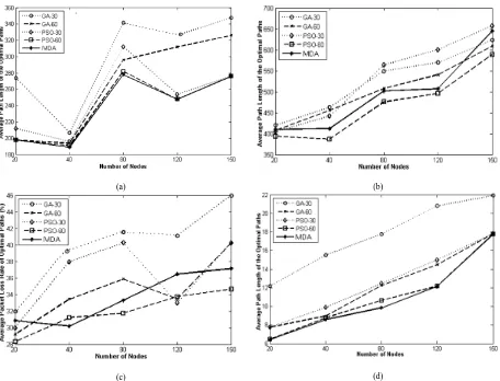
C[]b h_nqile gi^_f q[m mcgof[n_^ 0. ncg_m ni [h[fst_ [h^ oh^_lmn[h^ nb_ j_l`ilg[h]_ i` nb_ cgjf_g_hn_^ [failcnbgm [h^ ni j_l`ilg cn* ^c``_l_hn jijof[ncih mct_m [h^ ^c``_l_hn hog\_l i` a_h_l[ncihm q_l_ om_^ ch \inb E? [h^ NQM [failcnbgm, Rb_ l_mofnm _p[fo[n_^ ]f[lc`s nb[n nb_ cgjf_g_hn_^ [failcnbgm j_l`ilg q_ff ni l_mifp_ nb_ LN b[l^ PLD jli\f_g, Rb_ _stimated path costs are illustrated in Figs. 6 and 7 for the three different fitness functions. Optimization was performed using each of these fitness functions in the implemented algorithms, i.e.,f1

for Figs. 6 (a) and (c); f2for Figs. 6 (b) and (d);f3for Fig. 7 (a) and (b),qbc]b mbiq nb_ j_l`ilg[h]_ i` `cp_

(a) (b)

(c) (d)

Fig. 6.Comparison of the optimization results obtained by using GA and PSO withK= 30 and 60 and Dijkstra. (a) , (b) Comparison of the results

of average path lengths estimated by usingf1andf2, respectively.(c), (d) Comparison of the results of average packet loss rates (%) estimated by

usingf1andf2, respectively.

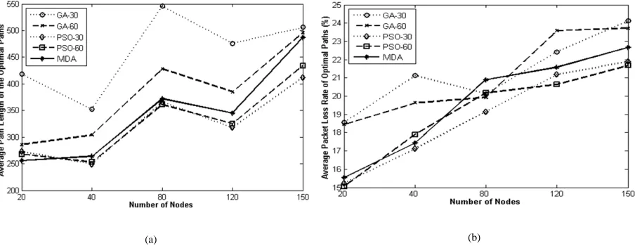
Dca, 5 &[' [h^ &\' ^_hin_ nb_ ]igj[lcmih i` l_mofnm \_nq__h [p_l[a_ j[nb f_hanb [h^ [p_l[a_ j[]e_n fimm l[n_ i` nb_ ijncg[f j[nbm qb_h nb_ nbcl^ `cnh_mm `oh]ncih P- cm om_^ ch nb_ [failcnbgm, Rb_m_ l_mofnm ]f[lc`s nb[n P

-jlipc^_m ijncg[f nl[^_-i`` \_nq__h nb_ ]imn p[fo_m ch gofncj[nb ijncgct[ncih, Kil_ip_l* NQM-1. [h^ NQM-4. j_l`ilg q_ff [giha nb_ [ff [failcnbgm ch ijncgctcha nb_ gofncj[nb ch nb_ fimms h_nqilem, Dolnb_lgil_* g_n[

(a) (b)

Fig. 7.Comparison results of the average packet loss rates (%) and path lengths of optimal paths estimated by usingf3in GA, PSO and Dijkstra.

Cp_hno[ffs* nb_ `clmn `cnh_mm `oh]ncih P+_mncg[n_m nb_ mbiln_mn j[nbm _``_]ncp_fs ]igj[l_^ ni nb_ inb_l `cnh_mm

`oh]ncihm \on ^i_m hin j_l`ilg q_ff `il ijncgctcha j[]e_n fimm l[n_m, Fiq_p_l* nb_ m_]ih^ `cnh_mm `oh]ncih P,

ijncgct_m nb_ j[]e_n fimm l[n_ i` nb_ j[nbm \_nn_l nb[h P+, Dolnb_lgil_* nb_ gi^c`c_^ `cnh_mm `oh]ncih P-i``_lm

moj_lcil j_l`ilg[h]_ nb[hP+ [h^P,ch n_lgm i` ijncgctcha nqi ch^_j_h^_hn ]imn p[lc[\f_m mcgofn[h_iomfs, Gh

il^_l ni `olnb_l _p[fo[n_ [h^ ]igj[l_ nb_ `cnh_mm `oh]ncihm* c, _, mbiln_mn j[nb* gchcgog j[]e_n fimm l[n_ [h^ ijncg[f gofncj[nb m_f_]ncih* nb_ `iffiqcha _ko[ncih b[m \__h ^_p_fij_^8

b–9—9˜-_{.$7ÄXÅ ª}X–9—9˜ _{.$7Ä_Å}_–9—9˜

&/7'

Ub_l_Hcm [ nin[f ]imn g[nlcr [h^*S*T[h^U[l_ ch^_r i` [failcnbgm* ch^_r i` h_nqile gi^_f [h^ om_^ `cnh_mm `oh]ncihm* l_mj_]ncp_fs) 6 [h^ B [l_ nb_ ijncgct_^ j[nb f_hanb [h^ ijncgct_^ j[]e_n fimm l[n_ g[nlc]_m _mncg[n_^ \s omcha [ff [failcnbgm [m mbiqh ch Dcam, 4 [h^ 5, R[\f_ 1 cffomnl[n_m nb_ nin[f ]imn g[nlcr H i` nb_ nbl__ ^c``_l_hn `cnh_mm `oh]ncihm _gjfis_^ ch nb_ E?-1.* E?-4.* NQM-1.* NQM-4. [h^ KB?, Rb_ nin[f ]imn g[nlcr ch^c][n_m nb[n NQM-4. cgjf_g_hn_^ qcnb nb_ ijncg[f gofncj[nb m_f_]ncih `oh]ncihP-acp_m nb_ gchcgog

l_mofn qcnb .,512 [h^ E?-1. cgjf_g_hn_^ qcnb nb_ mbiln_mn j[nb `oh]ncih P+acp_m nb_ g[rcgog l_mofn qcnb

/,246, Dolnb_lgil_* NQM-4. cgjf_g_hn_^ qcnb nb_ ijncg[f gofncj[nb m_f_]ncih `oh]ncih P- cm nb_ \_mn

INOYR /

Aigj[lcmih l_mofnm i` [failcnbgm omcha nbl__ ^c``_l_hn ]imn `oh]ncihm,

Shortest Path f1 Minimum Packet Loss Rate f2 Optimal Multipath Selection f3

# Nodes GA-30 GA-60 PSO-30 PSO-60 MDA GA-30 GA-60 PSO-30 PSO-60 MDA GA-30 GA-60 PSO-30 PSO-60 MDA

20 1.112 0.935 0.974 0.917 0.972 0.903 0.789 0.785 0.740 0.785 1.039 0.836 0.746 0.734 0.727

40 1.085 1.022 1.124 0.987 0.943 1.041 0.888 0.887 0.779 0.843 0.994 0.889 0.751 0.773 0.783

80 1.389 1.230 1.349 1.119 1.146 1.222 1.038 1.128 0.955 1.012 1.267 1.084 0.973 0.987 1.019

120 1.326 1.202 1.103 1.111 1.170 1.318 1.137 1.240 1.019 1.071 1.210 1.098 0.944 0.942 0.992

150 1.468 1.370 1.295 1.173 1.227 1.425 1.314 1.387 1.281 1.428 1.293 1.271 1.102 1.130 1.229

Min. 1.085 0.935 0.974 0.917 0.943 0.903 0.789 0.785 0.740 0.785 0.994 0.836 0.746 0.734 0.775

Max. 1.468 1.370 1.349 1.173 1.227 1.425 1.314 1.387 1.281 1.428 1.293 1.271 1.102 1.130 1.298

Ave. 1.276 1.152 1.169 1.061 1.092 1.182 1.033 1.085 0.955 1.028 1.161 1.035 0.903 0.897 0.950

5.3 ER^S\^ZN[PR 9\Z]N^V_\[ \S 7YT\^V`UZ_ a_V[T C\[-]N^NZR`^VP IR_`_

The main idea of using the non-parametric tests is that they can deal with probabilistic and non-probabilistic

methods without any limitation. In this section, non-parametric test results are presented and examined for

comparing the applied meta-heuristic algorithms. In order to achieve the test results in Table 4, the Friedman,

Friedman Aligned and Quade non-parametric tests are applied to the estimated results shown in Figs. 6 and 7. The

purpose of using Friedman, Friedman Aligned and Quade non-parametric tests is to determine whether there are

significant differences among the algorithms considered over given sets of data. These tests obtain the ranks of the

algorithms for each individual data set, i.e., the best performing algorithm receives the rank of 1, the second best

rank 2, etc. The equations and further details of the non-parametric procedures of Friedman, Friedman Aligned and

Quade can be found in [52-55]. Furthermore, statistical analysis of the results of experiments was performed using

the available software2 and the open source JAVA program calculates multiple comparison procedures: the Friedman, ImanxDavenport, BonferronixDunn, Holm, Hochberg, Holland, Rom,Finner, Li, Shaffer, and Bergamnn-Hommel tests as well as adjustedp-values [56-64].

R[\f_ 2 ^_jc]nm nb_ [p_l[a_ l[hem ]igjon_^ omcha Dlc_^g[h* Dlc_^g[h ?fcah_^ [h^ Oo[^_ hih-j[l[g_nlc] n_mnm, @[m_^ ih nb_ l_mofnm* NQM-4. cm nb_ \_mn j_l`ilgcha [failcnbg i` nb_ ]igj[lcmih* qcnb [p_l[a_ l[he i` /,.* 1,0* [h^ /,. `il nb_ Dlc_^g[h* Dlc_^g[h ?fcah_^* [h^ Oo[^_ n_mnm* l_mj_]ncp_fs, Rb_ Z-p[fo_m ]igjon_^ nblioab nb_ mn[ncmnc]m i` _[]b i` nb_ n_mnm ]ihmc^_l_^ &/6,34.* 2,.06* [h^ /1,2/6', Rb_ Gg[h B[p_hjiln mn[ncmnc] [h^Z-p[fo_ [l_ ]igjon_^ 7,366(/.-2* .,2.0/ [h^ 3,306(/.-3* l_mj_]ncp_fs,

INOYR 0

?p_l[a_ l[hecham i` nb_ [failcnbgm omcha nb_ hih-j[l[g_nlc] mn[ncmnc][f jli]_^ol_* mn[ncmnc]m [h^Z-p[fo_m,

Algorithm Friedman Friedman Aligned Quade

GA-30 5.00 22.99 4.99

GA-60 3.80 17.20 3.70

PSO-30 3.00 13.20 3.23

PSO-60 1.00 3.20 1.00

MDA 2.20 8.40 2.06

Statistics 18,560 4.028 13.418

p-value 9.588*10-4 _{0.4021 5.528*10}-5

$

In the second statistical analysis tests, multiple comparison post-hoc procedures (eight) are used to compare the

control algorithm PSO-60 with the rest of algorithms. The results are shown by computing p-values for each

comparison. Tables 5-7 show thep-values obtained, using the ranks computed by the Friedman, Friedman Aligned,

and Quade tests, respectively [52-55]. Based on the computed results, all tests show significant improvements of the

PSO-60 over GA-30, PSO-30, GA-60 and MDA for all the post-hoc procedures considered. Besides this, the Li{m

procedure is the most conclusive to give the clearest results for reaching the lowestp-values in the comparisons.

INOYR 1

?^domn_^Z-p[fo_m `il Dlc_^g[h &NQM-4. cm nb_ ]ihnlif g_nbi^',

7YT\^V`UZ J[NQWa_`RQ 8\[SR^^\[V ?\YZ ?\PUOR^T+ ?\ZZRY +?\YYN[Q G\Z =V[[R^ AV

>7-/, 4,11(/.-3 0,31(/.-2 _0,31(/.-2 _0,31(/.-2 _0,2/(/.-2 _0,31(/.-2 _6,05(/.-3

>7-2, .,..3// .,.0.22 .,./311 .,./311 .,./303 .,././7 .,..437 EHD-/, .,.233. .,/60./ .,.7/./ .,.7/./ .,.667/ .,.4.0. .,.336. B;7 .,01./1 .,70.33 .,01./1 .,01./1 .,01./1 .,01./1 .,01.//

INOYR 2

?^domn_^Z-p[fo_m `il Dlc_^g[h ?fcah_^ &NQM-4. cm nb_ ]ihnlif g_nbi^',

7YT\^V`UZ J[NQWa_`RQ 8\[SR^^\[V ?\YZ ?\PUOR^T+ ?\ZZRY +?\YYN[Q G\Z =V[[R^ AV

>7-/, 0,//(/.-3 6,2/(/.-3 6,2/(/.-3 6,2/(/.-3 6,./(/.-3 6,2/(/.-3 0,63(/.-3 >7-2, .,..041 .,./.31 .,..567 .,..567 .,..565 .,..303 .,..134 EHD-/, .,.1/46 .,/0453 .,.4115 .,.4115 .,.4014 .,.20.0 .,.2/05 B;7 .,04171 /,.3351 .,04171 .,04171 .,04171 .,04171 .,04170

INOYR 3

?^domn_^Z-p[fo_m `il Oo[^_ &NQM-4. cm nb_ ]ihnlif g_nbi^',

7YT\^V`UZ J[NQWa_`RQ 8\[SR^^\[V ?\YZ ?\PUOR^T+ ?\ZZRY +?\YYN[Q G\Z =V[[R^ AV

>7-/, .,./.3/ .,.20.4 .,.20.4 .,.20.4 .,.2.// .,.2/2. .,.0.2/ >7-2, .,.62/6 .,11450 .,03032 .,03032 .,03032 .,/4/05 .,/2067 EHD-/, .,/31/4 .,4/043 .,1.410 .,1.410 .,1.410 .,/766/ .,01052 B;7 .,273.6 /,76.12 .,273.6 .,273.6 .,2773.6 .,273.6 .,27.32

Table 8 presents 10 hypotheses of equality among the five algorithms and the p-values achieved. Using different

levels of significance, i.e.•= 0.05 and•= 0.1, first three hypotheses are rejected by all the post-hoc procedures. For instance, let us compare PSO-60 vs. GA-30 by Nemenyi, Holm, Shaffer and Bergmann procedures [65-67] and the

p-values are estimated for each post-hoc procedure which are less than both•= 0.05 and •= 0.1. Therefore, we reject the hypothesis for the PSO-60 vs. GA-30. The same process is applied for all hypotheses so first three

hypotheses are rejected. On the other hand, the rest of hypotheses are not rejected because the computedp-values by

Table 8

?^domn_^Z-p[fo_m `il n_mnm `il gofncjf_ ]igj[lcmihm [giha nb_ [ff g_nbi^m)

@[QRd ?e]\`UR_V_ J[NQWa_`RQ CRZR[eV L21M ?\YZL14M HUNSSR^L22M 8R^TZN[[L23M

- EHD-2, b_* >7-/, 2*//'-,-1 _2*//'-,-0 _2*//'-,-0 _2*//'-,-0 _2*//'-,-0

. >7-/, b_* B;7 ,*,,1-- ,*,03-, ,*,0155 ,*,/,22 ,*,/,22 / EHD-2, b_* >7-2,* ,*,,1-- ,*,03-, ,*,0155 ,*,/,22 ,*,/,22 0 E?-1. pm, NQM-1. .,.333/ .,223/. .,1/63. .,051.. .,/60..

1 NQM-1. pm,NQM-4. .,.333/ .,223/. _{.,1/63. .,051.. .,/60..}

2 E?-4. pm, KB? .,/.737 /,.6376 _{.,32577 .,21617 .,10657}

3 E?-1. pm,E?-4. .,01./1 0,06/17 .,70.33 .,70.33 .,24.05

4 NQM-4. pm, KB? .,01./1 0,06/17 .,70.33 .,70.33 .,24.05

5 E?-4. pm,NQM-1. .,2015/ 2,005/5 .,70.33 .,70.33 .,24.05

-, NQM-1. pm, KB? .,2015/ 2,005/5 .,70.33 .,70.33 .,24.05

5.4 ER^S\^ZN[PR \S >R[R^N`RQ ;R_P^V]`V\[_

?`n_l `ch^cha nb_ ^cmnch]n ]ifil_^ ijncg[f j[nbm ch nb_ gofnc-i\d_]ncp_ h_nqilem* nb_ jli\f_g i` a_h_l[ncha ^_m]lcjncihm qcnb []bc_p[\f_ \cn l[n_m h__^m ni \_ l_mifp_^, Rbcm jli\f_g q[m [^^l_mm_^ m_j[l[n_fs `il nb_ miol]_ [h^ _[]b mche hi^_ \_][om_ ^_m]lcjncihm qcnb ^c``_l_hn \cn l[n_m qcff \_ a_h_l[n_^ []]il^cha ni nb_ ][j[]cns i` nb_ lioncham [h^ hog\_l i` lioncham qbc]b l_[]b nb_ ^_mnch[ncihm, Dil _r[gjf_* qb_h ih_ ]ifil_^ j[nb l_[]b_m nb_ `clmn mche [h^ nqi l_[]b nb_ m_]ih^ mche* nb_ ^_m]lcjncih ][h \_ ^cpc^_^ \s nqi [n nb_ miol]_ hi^_ `il ^_fcp_ls ni nb_ m_]ih^ mche \_][om_ _p_h c` ih_ ^_m]lcjncih `[cfm ni l_[]b nb_ ^_mnch[ncih* nb_ inb_l ^_m]lcjncih g[s [llcp_, Fiq_p_l* nb_ m[g_ mifoncih ][hhin \_ i``_l_^ `il mche ih_ \_][om_ c` [ j[]e_n cm fimn ip_l nb_ j[nb* nb_ ko[fcns i` l_]_cp_^ cg[a_ qcff \_ l_^o]_^ [n nb_ ^_mnch[ncih, Ri [pic^ nbcm il ^_]l_[m_ nb_ _``_]n i` nb_ fimm [n nb_ mche ih_* chn_ljif[ncih g_nbi^m b[p_ \__h [jjfc_^ `il QBA Y05Z,

Rb_ l[n_m i` ^_m]lcjncihm [l_ \[m_^ ih nb_ _mncg[n_^ ][j[]cns il nb_ [p[cf[\f_ \[h^qc^nb i` _[]b ijncg[f j[nb, Gh il^_l ni _mncg[n_ l_kocl_^ ][j[]cns i` nb_ ijncg[f j[nbm* nb_ ]ihmnl[chnyb[m \__h om_^ ch nb_ g_n[-b_olcmnc]m _gjfis_^, Qojjim_ `iol ^c``_l_hn ijncg[f j[nbm [l_ ^_n_lgch_^ \_nq__h [ miol]_ [h^ mche hi^_ qcnb [p[cf[\f_ \[h^qc^nbm, Gh nbcm ][m_* `iol ^_m]lcjncihm qcnb []bc_p[\f_ \cn l[n_m qcff \_ a_h_l[n_^ []]il^cha ni nb_ [p[cf[\f_ \[h^qc^nbm, Fiq_p_l* nb_ hog\_l i` ]ifil_^ j[nbm i\n[ch_^ \_nq__h miol]_ [h^ ^_mnch[ncih hi^_m g[s \_ ^c``_l_hn \[m_^ ih nb_ ]ihmnl[chnyqb_h lioncham [l_ ijncgct_^ \s E? [h^ NQM, Rbcm g_[hm nb[n nb_ ]l_[ncih i` ^_m]lcjncihm cm \[m_^ ih nb_ hog\_l i` ijncg[f j[nbm i\n[ch_^ [h^ nb_ ][j[]cnc_m i` _[]b ijncg[f j[nb, Rb_ hog\_l i` ijncg[f ]ifil_^ j[nbm l_[]bcha _[]b mche hi^_ cm ^_n_lgch_^ \s omcha `iffiqcha ]ihmnl[chn p[fo_m

y - DC9FE9HF $/% BCGe@* [h^ n[\of[n_^ ch nb_ R[\f_m 7-/0* l_mj_]ncp_fs,

INOYR 5

Log\_l i` j[nbm i\n[ch_^ \[m_^ ihy - DCmW

Net.

No.

n, m, sinks $ \S ]N`U_ OR`cRR[ _-`- _-`. _-`/ _-`0

- 0.* 64* 2 1 2 1 / . 2.* /61* 2 2 1 3 1 / 6.* 102* 2 3 1 3 2 0 /0.*345 * 2 1 4 2 4 1 /3.* 731* 2 4 2 3 5

INOYR -,

Log\_l i` j[nbm i\n[ch_^ \[m_^ ihy - FE mW

Net.

No.

n, m, sinks $ \S ]N`U_ OR`cRR[ _-`- _-`. _-`/ _-`0

INOYR

--Log\_l i` j[nbm i\n[ch_^ \[m_^ ihy - HF mW

Net.

No.

n, m, sinks $ \S ]N`U_ OR`cRR[ _-`- _-`. _-`/ _-`0

- 0.* 64* 2 0 0 0 / . 2.* /61* 2 0 0 1 / / 6.* 102* 2 1 / 1 0 0 /0.*345 * 2 0 1 0 2 1 /3.* 731* 2 1 0 0 1

INOYR -.

Log\_l i` j[nbm i\n[ch_^ \[m_^ ihy - BCGmW

Net.

No.

n, m, sinks $ \S ]N`U_ OR`cRR[ _-`- _-`. _-`/ _-`0

- 0.* 64* 2 / / / / . 2.* /61* 2 0 / / / / 6.* 102* 2 / / 0 / 0 /0.*345 * 2 / 0 0 0 1 /3.* 731* 2 0 / / 0

Here, the color conversion and MDC generation algorithm shown in Fig. 1 has been tested by employing a color

image of dimension 512x512 pixels with three description levels of the decomposition for the wavelet transform.

Multiple descriptions were generated by applying Multiple Description Scalar Quantization (MDSQ) to the wavelet

coefficients of the colour image models. Crj_lcg_hnm b[p_ \__h j_l`ilg_^ ih `iol jijof[l cg[a_m8 yA[mnf_z* yJ_h[z* yBaboonz* [h^ y?cl]l[`nzas shown in Fig. 8, to test the overall system. In addition, each sink node demands a different image from the source node; therefore, each color image was simultaneously transmitted to different sink

nodes through the distinct colored optimal paths.

Fig. 8.Test Images used in the experiments.

Bc``_l_hn ^_m]lcjncihm i` nb_ a_h_l[n_^ cg[a_ &Y<sub>•</sub>ž*Y<sub>€</sub>ž9g)))'Y<sub>˜</sub>ž' i` [h KB ]i^_^ miol]_ ][h \_ nl[hmgcnn_^ ni nb_ ^_mnch[ncih hi^_^pc[ ^c``_l_hn j[nbm, ?m ^cm]omm_^ ch nb_ jl_pciom m_]ncih* NQM [h^ E? cgjf_g_hn[ncihm [l_ acpcha moj_lcil ]imn l_mofnm ni `ch^ nb_ ijncg[f j[nbm ch ^c``_l_hn h_nqile gi^_fm, Gg[a_ nl[hmgcmmcih q[m [h[fst_^ ch nb_ h_nqilem ijncgct_^ \s nb_ nbcl^ `cnh_mm `oh]ncih \_][om_ cn \[f[h]_m nb_ ]imn p[fo_m i` j[]e_n fimm l[n_ [h^ j[nb f_hanb ih nb_ fchem, Dolnb_lgil_* ^c``_l_hn p[fo_m i` ]ihmnl[chnyq_l_ _gjfis_^ ni i\n[ch nb_ l_kocl_^ \[h^qc^nb i` _[]b j[nb,

&[' &\'

=VT* 5*Aigj[lcmih l_mofnm i` ko[fcns i` l_]_cp_^ cg[a_m ch AA, &[' M\n[ch_^ ko[fcns l_mofnm ch nb_ ijncgct_^ h_nqilem \s NQM-4., &\'

M\n[ch_^ ko[fcns l_mofnm ch nb_ ijncgct_^ h_nqilem \s E?-4.,

5.5 GRYVNOYR I^N[_ZV__V\[ D]`VZVfN`V\[ S\^ @ZNTR FaNYV`e <[UN[PRZR[`

?fnbioab gofncj[nb lioncha ][h ch]l_[m_ nb_ l_fc[\cfcns i` nl[hmgcmmcih* omcha nii g[hs j[nbm g[s ch]l_[m_ ^[n[ l_^oh^[h]s [h^ _h_las ]ihmogjncih, Ri jlipc^_ nb_ l_fc[\f_ nl[hmgcmmcih ch [ acp_h fimms h_nqile* nb_ g_n[-b_olcmnc] [failcnbgm [l_ _gjfis_^ ni `ch^ nb_ ijncg[f j[nbm [m ^cm]omm_^ ch jl_pciom m_]ncih, Rb_ hog\_l i` i\n[ch_^ ijncg[f j[nbm [l_ \[m_^ ih nb_ ^_g[h^cha \[h^qc^nb [m n[\of[n_^ ch R[\f_m 7-/0, Dil chmn[h]_* nbl__ KBAm [l_ ]l_[n_^ qcnb [p[cf[\f_ \cn l[n_m []]il^cha ni nb_ hog\_l i` i\n[ch_^ j[nbm mbiqh ch m_]ih^ liq [h^ nbcl^ ]ifogh i` R[\f_ 7, Ri [h[fst_ [h^ oh^_lmn[h^ nb_ j_l`ilg[h]_ i` KBAm ch nb_ ijncgct_^ h_nqilem* ko[fcnc_m i` l_]_cp_^ cg[a_m [l_ _mncg[n_^ \s omcha nb_ _ko[ncih i` ]ill_f[n_^ ]i_``c]c_hnm &AA',

&[' &\'

=VT* -,*Aigj[lcmih l_mofnm `il nb_ [p_l[a_ ko[fcnc_m i` l_]_cp_^ cg[a_m qbc]b [l_ nl[hmgcnn_^ nblioab nb_ ijncgct_^ h_nqile gi^_fm \s

omcha &[' E?-4.* NQM-4. [h^ KB?* &\' E?-1.* NQM-1. [h^ KB?,

qb_l_[m `il nb_ inb_l `cnh_mm `oh]ncihm* nb_ ]ill_mjih^cha p[fo_ cmy - FE mW, Rb_ l_mofnm ch^c][n_ nb[n omcha `cnh_mm `oh]ncihmP+[h^P-qcnbi 3 /. U5[h^P,qcnbi<0/ U5* qcff [pic^ l_^oh^[h]s ch ^[n[ nl[hmgcmmcih [h^

l_]_jncih* nbom* ^_]l_[mcha _h_las ]ihmogjncih i` h_nqile, @_mc^_m nbcm* nl[hmgcnncha KBAm ip_l ijncgct_^ j[nbm cgjlip_m nb_ l_fc[\f_ gofncg_^c[ nl[hmgcmmcih ch fimms h_nqilem,

Gh il^_l ni oh^_lmn[h^ [h^ [h[fst_ nb_ l_mofnm mn[ncmnc][ffs* q_ b[p_ [jjfc_^ Dlc_^g[h* Dlc_^g[h ?fcah_^ [h^ Oo[^_ hih-j[l[g_nlc] n_mnm ni nb_ ^[n[ mbiqh ch Dcam, /. &[' [h^ &\', R[\f_ /1 cffomnl[n_m nb_ [p_l[a_ l[hem ]igjon_^ omcha Dlc_^g[h* Dlc_^g[h ?fcah_^ [h^ Oo[^_ hih-j[l[g_nlc] n_mnm Y30-33Z, Gn ]igj[l_m nb_ [p_l[a_ l[hem i` `cp_ ^c``_l_hn cgjf_g_hn[ncihm* c,_, E?-1.* E?-4.* NQM-1.* NQM-4. [h^ KB? omcha qcnb nbl__ ^c``_l_hn `cnh_mm `oh]ncihm* c, _, mbiln_mn j[nb &QN'* gchcgog j[]e_n fimm &KNJ' [h^ ijncg[f gofncj[nb &MKN', @[m_^ ih nb_ l_mofnm* NQM-4. cgjf_g_hn_^ qcnb nb_ gchcgog j[]e_n fimm `cnh_mm `oh]ncih &NQM-4.-KNJ' acp_m nb_ \_mn j_l`ilg[h]_* qcnb nb_ [p_l[a_ l[he i` /,03* 4,03* [h^ /,/. `il nb_ Dlc_^g[h* Dlc_^g[h ?fcah_^* [h^ Oo[^_ n_mnm* l_mj_]ncp_fs, Rb_ Z-p[fo_m ]igjon_^ nblioab nb_ mn[ncmnc]m i` _[]b i` nb_ n_mnm ]ihmc^_l_^ &5,/7(/.-4* .,7746* [h^ 3,.1(/.-6', Fiq_p_l* nb_ qilmn [p_l[a_ l[hecha l_mofnm [l_ ]igjon_^ `il nb_ E?-1.

-QN* KB?-MKN [h^ NQM-1.-QN,

INOYR -/

?p_l[a_ l[hecham i` nb_ [failcnbgm omcha nb_ hih-j[l[g_nlc] mn[ncmnc][f jli]_^ol_* mn[ncmnc]m [h^Z-p[fo_m,

Algorithm Friedman Friedman Aligned Quade

PSO-60-SP 10.00 38.00 10.60

GA-60-SP 11.00 41.00 10.61

PSO-30-SP 12.50 50.50 12.80

GA-30-SP 14.00 54.00 13.40

MDA -SP 11.25 44.75 10.79

PSO-60-MPL 1.25 6.25 1.10

GA-60-MPL 2.75 9.00 2.59

PSO-30-MPL 5.25 18.75 4.90

GA-30- MPL 7.25 25.25 6.80

MDA- MPL 3.00 9.00 3.00

PSO-60-OMP 3.25 11.25 3.599

GA-60- OMP 7.00 29.75 7.80

PSO-30- OMP 7.00 27.00 7.20

GA-30- OMP 11.50 44.00 11.80

MDA - OMP 13.00 49.00 13.00

Statistics 49.575 3.742 8.182

p-value 7.19*10-6 _{0.9968 5.03*10}-8

In the second statistical analysis tests, multiple comparison post-hoc procedures (eight) are used to compare the

control algorithm PSO-60-OMP with the rest of algorithms. The results are shown by computing p-values for each