promoting access to White Rose research papers
White Rose Research Online
Universities of Leeds, Sheffield and York
http://eprints.whiterose.ac.uk/
This is an author produced version of a paper published in
Combustion theory
and modelling.
White Rose Research Online URL for this paper:
http://eprints.whiterose.ac.uk/3683/
Published paper
Sharpe, G.J. (2003)
Linear stability of planar premixed flames: reactive
Navier-Stokes equations with finite activation energy and arbitrary Lewis number,
Combustion theory and modelling, Volume 7 (1), 45-65.
Linear stability of planar premixed flames: Reactive
Navier-Stokes equations with finite activation
energy and arbitrary Lewis number
G J Sharpe†
School of Mathematics and Statistics, University of Birmingham, Edgbaston, Birmingham, B15 2TT, UK
Abstract. A numerical shooting method for performing linear stability analyses of travelling waves is described and applied to the problem of freely propagating planar premixed flames. Previous linear stability analyses of premixed flames either employ high activation temperature asymptotics or have been performed numerically with finite activation temperature, but either for unit Lewis numbers (which ignores thermal-diffusive effects) or in the limit of small heat release (which ignores hydrodynamic effects). In this paper the full Reactive Navier-Stokes equations are used with arbitrary values of the parameters (activation temperature, Lewis number, heat of reaction, Prandtl number), for which both thermal-diffusive and hydrodynamic effects on the instability, and their interactions, are taken into account. Comparisons are made with previous asymptotic and numerical results. For Lewis numbers very close to or above unity, for which hydrodynamic effects caused by thermal expansion are the dominant destablizing mechanism, it is shown that slowly varying flame analyses give qualitatively good but quantitatively poor predictions, and also that the stability is insensitive to the activation temperature. However, for Lewis numbers sufficiently below unity for which thermal-diffusive effects play a major role, the stability of the flame becomes very sensitive to the activation temperature. Indeed, unphysically high activation temperatures are required for the high activation temperature analysis to give quantitatively good predictions at such low Lewis numbers. It is also shown that state-insensitive viscosity has a small destabilizing effect on the cellular instability at low Lewis numbers.
1. Introduction
A premixed flame is a slow (subsonic) combustion wave which propagates via conduction of heat and diffusion of chemical species between the hot burnt products and the cold unburnt fuel. While flames may propagate as planar and steady waves, experiments show that in many cases the flame is wrinkled and possibly time-dependent (Buckmaster & Ludford 1982; Sivashinsky 1983; Strehlow 1985), so called ‘cellular’ flames. A first step in understanding the origins of these multi-dimensional flames is a linear stability analysis of the underlying steady, planar wave. The linear stability of premixed flames dates back to the Landau-Darrieus analysis (Landau & Lifshitz 1959), which treats the flame as a discontinuity that separates inert hydrodynamic flows. This analysis predicts that the growth rate of perturbations is inversely proportional to the wavelength of the perturbation, contrary to experimental
results. Later, high activation temperature asymptotic analyses were employed, in which the reaction zone is still treated as a discontinuity, the ‘flame sheet’, but the structure of the diffusive pre-heat zone is taken into account. Sivashinsky (1977) used the constant density approximation (CDA), which completely ignores hydrodynamic effects and is formally valid in the limit of small heat release. He showed that for Lewis numbers (ratio of thermal to species diffusivities) sufficiently less than unity, thermal-diffusive effects alone are sufficient to cause the cellular instability. He also found a pulsating instability for Lewis numbers sufficiently above unity. However this pulsating instability regime is outside the normal parameters, and hence not attainable, for adiabatic flames in gases (Joulin & Clavin 1979; Pelce & Clavin 1982; Sivashinsky 1983) (large enough heat losses can make premixed flames unstable to the pulsating instability (Joulin & Clavin 1979; Jackson & Kapila 1986; Buckmaster 1983), but such effects are not considered here). Frankel & Sivashinsky (1982), Matalon & Matkowsky (1982) and Pelce & Clavin (1982) performed slowly-varying flame (SVF) analyses in which the wavelength of the perturbation is assumed to be much longer than the flame thickness (note that in this paper we follow the notation used in Jackson & Kapila (1986), i.e. we use the term SVF to describe a flame varying over length and time scales much longer than the diffusive scales, a more formal definition of SVF’s is given in Buckmaster & Ludford (1982)). They showed that for Lewis numbers sufficiently close to or above unity, the primary instability mechanism is due to hydrodynamic effects (thermal expansion caused by the heat release). The SVF analysis also provides higher order corrections to the Landau-Darrieus result, which show that there is wavelength for which the growth rate is maximum and that the flame is stable for sufficiently small perturbation wavelengths. Jackson & Kapila (1984, 1986) then solved numerically the leading order linearized equations in the infinite activation temperature limit, but made no assumptions about the size of the heat release or wavelength of the perturbation. They showed that even for Lewis numbers less than unity, hydrodynamic effects still play a major role.
realistic, activation temperatures can give results which are qualitatively different than the predictions of an infinite activation temperature asymptotic analysis (e.g Shah, Thatcher & Dold (2000) for flame balls or Singh & Clarke (1992) for shock ignition of detonations). Hence it is important to check the validity of the asymptotic linear stability results, and also the validity of the other asymptotic approximations made (the limits of small heat release in the CDA analysis and small wavenumber in the SVF analysis), for realistic parameter values. Also, the high activation temperature asymptotic results mentioned above all assume that the Lewis number is asymptotically close to one, i.e. near-equidiffusional flames (NEFs). However, the Lewis number can vary between about 0.3 for hydrogen (Short, Buckmaster & Kochevets 2001) to 1.8 for propane (Pelce & Clavin 1982), and hence a method is required for determining the stability of flames with Lewis numbers O(1) different from unity.
Secondly, a numerical method needs to be developed for determining the linear stability of flames, which can, in principal, be applied to more complex flame models for which an asymptotic stability analysis of the Reactive Navier-Stokes equations may not be straightforward or possible, e.g. for simple two- or three-step chain-branching models (Doldet al. 2002, Gasser & Szmolyan 1995), or even for complex chemistry, in which some of the activation temperatures of the reactions may be moderate or small. Indeed for chain-branching chemistry, the chain-termination steps, which release most of the heat (Short & Quirk 1997) usually have very weak temperature dependences (low activation temperatures) and hence a high activation temperature analysis is not appropriate for these reactions, so that for chain-branching models the exothermic reaction zones cannot be reduced to thin sheets (Buckmaster & Ludford 1982).
(1995) found a different dependence on the activation temperature in their Reactive Navier-Stokes simulations of hydrodynamically dominated flame instabilities than Fr¨olich & Peyret (1991). Denet & Haldenwang (1995) suggest this is because Fr¨olich & Peyret (1991) use a numerical mesh that does not provide enough resolution in the reaction zone at higher activation temperatures. However, comparisons with a linear stability analysis for finite activation temperature will determine which, if either, of the results of Denet & Haldenwang (1995) or Fr¨olich & Peyret (1991) are correct, and hence which numerical scheme is more appropriate for nonlinear flame stability calculations.
While the numerical shooting method is developed here is described in the context of the stability of freely propagating planar flames, it can be implemented to determine the linear stability of many other travelling waves solutions, such as reaction-diffusion fronts (Zhang & Falle 1994; Gubernovet al. 2001). A version of it has already been applied to the stability of detonation waves (Sharpe 1997a, 1999). This method is an alternative to compound matrix methods for eigenvalue problems of systems of ordinary differential equations (Ng & Reid 1985; Gubernovet al. 2001; Lasseigneet al. 1999).
In§2 we give the governing equations and non-dimensionalization. The steady, one-dimensional waves are then considered in§3. The linearized equations are derived in§4 and the numerical shooting method described in§5. The results and conclusions, together with suggestion for future work, are given in§6 and§7, respectively.
2. Governing equations
The governing equations of the model are the Reactive Navier-Stokes equations for a single reaction A→B. The dimensionless versions of these equations are, in two-dimensions,
∂ρ ∂t +
∂(ρu)
∂x + ∂(ρv)
∂y = 0 (1)
ρ∂u ∂t +ρu
∂u ∂x+ρv
∂u ∂y+
∂P ∂x =Pr
4 3
∂2u
∂x2 +
∂2u
∂y2 +
1 3
∂2v
∂x∂y
(2)
ρ∂v ∂t +ρu
∂v ∂x+ρv
∂v ∂y +
∂P ∂y =Pr
4
3
∂2v
∂y2 +
∂2v
∂x2 +
1 3
∂2u
∂x∂y
(3)
ρ∂T ∂t +ρu
∂T ∂x +ρv
∂T ∂y +Q
ρ∂Y
∂t +ρu ∂Y
∂x +ρv ∂Y ∂y = Q Le ∂2Y
∂x2 +
∂2Y
∂y2
+∂
2T
∂x2 +
∂2T
∂y2 (4)
ρ∂Y ∂t +ρu
∂Y ∂x +ρv
∂Y ∂y =
1 Le
∂2Y
∂x2 +
∂2Y
∂y2
+W (5)
ρT = 1. (6)
W the reaction rate. These equations have been non-dimensionalize in the following way:
ρ= ρ¯ ¯
ρf
, u= u¯¯
Vf
, v= ¯v¯
Vf
, p= p¯ ¯
pf
, T = p
ρ=
¯
T
¯
Tf
,
x= ρ¯fV¯f¯cp ¯
κ x,¯ y=
¯
ρfV¯fc¯p ¯
κ y,¯ t=
¯
ρfV¯f2c¯p ¯
κ ¯t,
where a bar ( ¯ ) denotes dimensional quantities, a zero (0) subscript denotes quantities in the steady, planar flame, an f subscript denotes quantities in the fresh, unburnt gas upstream of the flame (and ab subscript will be used to denote quantities in the completely burnt state downstream of the flame). Here ¯Vf is the speed of the steady, planar flame, ¯cpis the specific heat at constant pressure, ¯κis the co-efficient of thermal conductivity and ¯ρfV¯fc¯p/κ¯is the lengthscale of the preheat zone in the steady, planar flame (Strehlow 1985).
The reaction rate is assumed to have an Arrhenius form, i.e.
W =−ΛρYe−θ/TH(T−Ti), (7)
where H is the Heaviside function. Here an ignition temperature Ti is specified, below which the reaction is switched off, to avoid the cold boundary difficulty (Williams 1985). The dimensionless parameters appearing in (2)-(5) and (7) are the Prandtl number, Pr = ¯µc¯p/κ¯ (ratio of viscous to thermal diffusivities), Lewis number,Le= ¯κ/(¯cpλ¯) (ratio of thermal to mass diffusivities), dimensionless activation temperature, θ = ¯θ/T¯f, and heat release, Q = ¯Q/(¯cpT¯f), and Λ = Da/Mf2 is the eigenvalue for the steady, planar flame speed, where Da is the Damk¨ohler number, Da = ¯kκ/¯ (γp¯f¯cp) (ratio of diffusion time to reaction time) and Mf is the Mach number of the flame,Mf = ¯Vf(¯ρf/(γp¯f))
1
2, withγ the ratio of specific heats. Here ¯µ and ¯λare the co-efficients of viscosity and species diffusion.
Note that θ is the dimensionless activation temperature scaled with the temperature in the fresh fuel. High activation temperature asymptotic analyses employ an alternative scaling for the activation temperature, namely the Zeldovich number,β, defined by
β =θ¯( ¯Tb¯−T¯f)
T2 b
= Qθ
(1 +Q)2, (8)
the asymptotic analyses then assumeβ is large.
Most flames travel at speeds from 1 to 100 cm s−1 (Williams 1985), so that they
propagate highly subsonically, Mf << 1. The process is then nearly isobaric. The quantityP appearing in (2) and (3) is theO(M2
f) deviation of the pressure from the upstream value, i.e. p= 1 +γM2
fP. Equations (1) to (6) are thus the leading order equations in an expansion inMf2(note that the viscous terms in the energy equation (4) areO(Mf2) and hence have been neglected). The system (1)-(6) are the standard model equations for premixed flames (e.g. Buckmaster & Ludford 1982).
3. Steady, planar flames
In the laboratory frame the steady, planar flame is assumed to travel in the negative
x-direction at unit speed in dimensionless variables, so that the fresh, unburnt fuel is approached as x → −∞ and the completely burnt state approached as x → ∞. However, the reactive Navier-Stokes equations are Galilean invariant. Hence we will consider them to be written in a frame moving with the steady flame. In this frame the flame is stationary, the flow is steady (independent of t) and the upstream fuel is moving at unit speed. After integrating once with respect tox and employing the boundary conditionsT0 =ρ0= u0 =Y0 = 1,P0 = 0 and dT0/dx = dY0/dx = 0 as
x→ −∞, (1)-(5) can be reduced to dT0
dx =T0−1 +Q(Z0−1),
dY0
dx =Le(Y0−Z0),
dZ0
dx =−
ΛY0
T0
e−θ/T0H(T0−Ti), (9)
where Z0 is a reaction progress variable defined by the second of (9) (Gasser &
Szmolyan 1993), and
u0=
1
ρ0
=T0, P0=
4Pr
3 (T0−1 +Q(Z0−1))−(T0−1). (10) In the fully burnt stateY0 = dY0/dx = dT0/dx = 0 so that (9)-(10) give the burnt
state asT0b =u0b = 1/ρ0b = 1 +Q, P0b =−Qas x → ∞. In order to satisfy both the boundary conditions asx → −∞ and x → ∞, Λ, which is related to the flame speed, must have a specific value. Hence Λ is the eigenvalue of (9) which needs to be determined numerically.
Equations (9) are autonomous and hence we can replace the independent variable
xwith one of the dependent variables. Here we choose the temperatureT0as the new
independent variable, so that the system to be solved is reduced to 2 equations:
dY0
dT0 =
Le(Y0−Z0)
T0−1 +Q(Z0−1),
dZ0
dT0 =−
ΛY0e−θ/T0H(T0−Ti)
T0(T0−1 +Q(Z0−1)).(11)
From a numerical perspective, this also has the advantage that an infinite domain
x∈(−∞,∞) is mapped onto a finite domainT0∈[1,1 +Q].
Note that for Le = 1, the first of (11) has the analytical solution Y0 =
[(1 +Q)−T0]/Q. Note also that for general Lewis numbers, in the region T0 ≤Ti,
Z0 = 1 and hence Y0 = 1−A(T0−1)Le, where A is a constant to be determined.
Now consider the solution of (11) close to the burnt state T0 = 1 +Q. Defining
wb = 1 +Q−T0, thenwb <<1,Y <<1 andZ <<1 sufficiently near the burnt state, and (11) linearize to
dY0
dwb
= Le(Y0−Z0)
wb−QZ0
, dZ0
dwb
= BY0
(wb−QZ0)
,
B =−Λe
−θ/(1+Q)
1 +Q . (12)
The solution to (12) which is bounded atwb= 0 is
Y0=
h0(1−h0)
QB wb, Z0=
(1−h0)
h0=
Le−(Le2−4LeB)12
2 . (13)
The numerical shooting method used to determine the eigenvalue Λ is as follows: for a given value of Λ, the asymptotic solutions (13) are used as initial conditions to start the integration of (11) near the burnt state, equations (11) are then integrated in the direction of decreasing T0 until T0 = Ti. If Z0 >1 at T0 = Ti then Λ is too high, whereas Λ is too low ifZ0<1 there. Hence one can iterate for Λ using bisection until
the required conditionZ0= 1 is satisfied atT0=Ti. As a good initial guess for Λ, the high activation temperature asymptotic result of Bush & Fendell (1970) is used. For moderate to high values ofθ, the Arrhenius term in the reaction rate is exponentially small nearT0=Ti providedTi is close to one and hence Λ is insensitive to the value ofTichosen (see§6.5) . Here we useTi = 1.01. Once the eigenvalue Λ has been found, the constant A can be determined using the value ofY0 found at T0 =Ti from the numerical integration. The spatial profiles can then also be determine by integrating dx/dT0 as an auxiliary equation. Note that the spatial origin is arbitrary. Here we
choosex = 0 to correspond to T0 = 1 +Q/2. We use a fourth-order Runge-Kutta
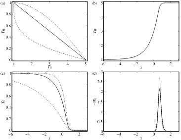
routine with adaptive step doubling to perform all the integrations in this paper. Figure 1 shows the steady, planar flame solutions forQ= 4,θ = 70 and various Lewis numbers, as well as forθ= 90 whenLe= 1. Note that the reaction occurs over a relatively thin zone. As the activation temperature increases the reaction zone becomes narrower and the maximum reaction rate increases (in the limitβ → ∞the reaction rate tends to a delta function). Note that increasing the activation temperature only effects the temperature profiles in the reaction zone, but not in the pre-heat zone. Note also the linear dependence ofY0 onT0 forLe= 1 in figure 1(a).
4. Linearized equations
We now suppose that the steady, planar flame is slightly perturbed such that the perturbations have the normal mode form
q(x, y, t) =q0(x) +q1(x)eσteiky, <<1, (14)
whereqis one ofT,u,v,P orY (note thatρ= 1/T from (6) so that the density can be eliminated from (1)-(5)),σ is the (complex) growth rate andkis the wavenumber of the disturbance in the y-direction. Note that out choice of a two-dimensional disturbance also covers the case of three-dimensional perturbations, since if we have a three-dimensional perturbation of the formq1(x)eσteik1yeik2z, we can choose a new
transverse directiony0
with wavenumberk= (k2 1+k22)
1 2. The reaction rateW is then expanded as
W =W0(x) +W0,TT1(x)eσteiky+W0,YY1(x)eσteiky+. . . , (15)
whereW0,T =∂W0/∂T0, etc. We then define the following quantities
τ1=
dT1
dx , U1=
du1
dx, V1=
dv1
dx, Z1=Y1−
1 Le
dY1
dx. (16)
Equations (14)-(16) are then substituted into the governing equations (1)-(5) and the result linearized in. Note first that (1) contains only firstx-derivatives and hence its linearized version can be used to eliminateτ1in terms of the other perturbed
quantities:
τ1=
(T0 0−σ)T1
T0
−T 0 0u1
T0
1 2 3 4 5 0
0.2 0.4 0.6 0.8 1
T0
Y0
(a)
−61 −4 −2 0 2
2 3 4 5
x
T0
(b)
−60 −4 −2 0 2
0.2 0.4 0.6 0.8 1
x
Y0
(c)
−60 −4 −2 0 2
0.5 1 1.5 2 2.5 3
x
−W
0
[image:9.612.97.463.49.332.2](d)
Figure 1. (a) Steady solutions in the (T0, Y0)-plane and spatial profiles of (b)
temperature, (c) fuel mass fraction and (d) reaction rate, for Q = 4, θ = 70 (β = 11.2) and Lewis numbers 0.3 (dashed lines), 1.0 (solid lines) and 1.8 (dot-dashed lines). Also shown are the profiles forθ= 90 (β= 14.4),Le= 1.0 (dotted lines).
where the prime denotes differentiation with respect tox. The linearized versions of equations (2)-(5), together with (16), can then be written in the form
du
dx =Au, (17)
whereu= (T1, u1, v1, P1, Y1, U1, V1, Z1)T and
(T0 0−σ)
T0
−T0 0
T0
ik 0
0 0 0 0
0 0 0 0
A41 A42 4ik
Pr(σ+T0−T00)
3T0
0
0 0 0 0
A61 −σT 0
0+T0T000
T2 0
ik(σ+T0−T00)
T0 0
0 0 3σ+ 4Prk
2T 0
3PrT0
ik
Pr
Y0
0+W0,TT0
T0
−Y0 0
T0
0 0
0 1 0 0
0 1 0 0
0 0 1 0
4PrQW0,Y 3
4Pr(σ+T0)−3T0
3T0 −ik
Pr 0
Le 0 0 −Le
QW0,Y
σ+T0
T0
−ik 0
0 ik
3
1
Pr 0
−Leσ−k2T
0+LeW0,YT0
LeT0 0 0 0
, where
A41=4
Pr(−σ2+T0
0σ+ (k2+QW0,T)T02−T0T000)
3T2 0 +T 0 0 T0 ,
A42=
−(4PrT0
0+ 3T0)σ
3T2 0
+Pr(4T 00
0 −3T0k2)
3T0
−T 0 0
T0
,
A61=(−σ 2+T0
0σ+ (k2+QW0,T)T02−T0T000)
T2 0
.
Note that thePr = 0 case investigated by Libermanet al. (1994) is a singular limit of (17). ForPr= 0,u00
1 andv 00
1 do not appear in the problem, and the corresponding
version of (17) is reduced to a 6×6 problem.
Since the steady structure is infinite in length it is again beneficial to useT0 as
the independent variable. Equation (17) then becomes
T0 0
du
dT0
= (T0−1 +Q(Z0−1))
du
dT0
=Au. (18)
The boundary conditions are that the solutions of (18) are bounded as T0 → 1
(x → −∞) and as T0 → 1 +Q (x → ∞). Only for certain, discrete values of the
5. Determining the growth rates
In this section we describe the numerical method for determining the eigenvalues of the growth rateσ. We first need to determine asymptotic solutions to (18) valid as the fresh state is approached (T0→1) and as the burnt state is approached (T0→1 +Q).
Note that T0
0 = 0 at T0 = 1 and at T0 = 1 +Q and hence these are both regular
singular points of (18).
Consider first the solutions near the fresh state,T0−1<<1. Definingwf =T0−1, we can expand the steady variables and hence A in terms of wf, recalling that
Y0= 1−AwLef , Z0= 1 forT0< Ti (i.e. for sufficiently smallwf), to give.
wf d
u
dwf
= (A0+A1wf+A2wLef +. . .)u, (19)
where the co-efficient matrices,A0, etc., depend only onPr, Le, k andσ. Note that
the ordering of the higher order terms in the expansion depends on whether Le is greater or less than unity (for Le = 1 the expansion for A is simply of the form
A0+A1wf+. . .). Equation (19) has 8 independent solutions of the form
ui=wfhi(ai0+ai1wf+ai2wLef +. . .), i= 1, . . . ,8 (20) where hi are the eigenvalues ofA0 andai0 are the corresponding eigenvectors. The
ai1,ai2, etc., are found by substituting (20) into (19) and equating powers ofwf. The eigenvalues ofA0 are
1±[1 + 4(σ+k2)]1 2
2 ,
Le±[Le2+ 4(σLe+k2)]1 2
2 ,
1±[1 + 4Pr(σ+Prk2)]1 2
2Pr , ±k. (21)
For Re(σ) ≥ 0 the eigenvalues with the negative signs have negative real part and correspond to unbounded solutions as wf → 0 and hence we must discard these solutions. We are thus left with 4 independent solutions corresponding to the positive signs in (21).
Now consider the solutions of (18) near the burnt state (T0→1 +Q). Expanding
the steady variables, and henceAin terms ofwb= 1 +Q−T0<<1 (see (13)) gives
h0wb d
u
dwb
= (A∗0+A∗1wb+. . .)u, (22)
where h0 is defined in (13), and now A∗0, etc., depend on Pr, Le, Q, θ, k and σ.
Equation (22) then has 8 independent solutions of the form
ui=w(h ∗
i/h0)
b (a
∗ i0+a
∗
i1wb+. . .), i= 1, . . . ,8 (23) where h∗
i are the eigenvalues of A ∗
0 anda∗i0 are the corresponding eigenvectors. The
eigenvalues ofA∗ 0 are
1±[1 + 4(σ/(1 +Q) +k2)]1 2
2 ,
Le±[Le2+ 4(σLe/(1 +Q) +k2−BLe)]1 2
2 ,
1±[1 + 4Pr(σ/(1 +Q) +k2Pr)]1 2
where B is defined in (12). Since h0 < 0, for Re(σ) ≥ 0, the eigenvalues with
positive signs in (24) give negative values ofh∗
i/h0and hence correspond to unbounded
solutions of (22) aswb →0, and these solutions must be discarded. Again, we are left with 4 independent solutions corresponding to the negative signs in (24).
We are now in a position to determine the eigenvalue growth rates σ using a numerical shooting method. For a given value of σ, the four bounded asymptotic solutions (20) valid asT0→1 are used as initial conditions to start the integration of
(18) away from the fresh state to the middle of the domain,T0 = 1 +Q/2. We then
have a general solution foruatT0= 1 +Q/2,
u=α1uf1+α2uf2+α3uf3+α4uf4,
whereufi,i= 1, . . . ,4, are the four solutions atT0= 1 +Q/2 found from using each of
the 4 bounded asymptotic solutions nearT0= 1 as initial conditions for the integration
and the αi are the corresponding (complex) constants of integration. Next, the four bounded asymptotic solutions (23) valid asT0→1 +Qare used as initial conditions
to start the integration of (18) away from the burnt state toT0= 1 +Q/2. We then
have a second general solution foruatT0= 1 +Q/2
u=α5ub1+α6ub2+α7ub3+α8ub4,
whereubi,i= 1, . . . ,4, are the four solutions at T0= 1 +Q/2 found from using each
of the 4 bounded asymptotic solutions near T0 = 1 +Qas initial conditions for the
integration andα5, . . . , α8 are (complex) constants of integration.
Ifσis an eigenvalue then the constantsα1, . . . , α8can be chosen so that the two
general solutions atT0= 1 +Q/2 match, i.e.
α1uf1+α2uf2+α3uf3+α4uf4 =α5ub1+α6ub2+α7ub3+α8ub4. (25)
Since we are interested in non-trivial solutions to (25), i.e. those for which not all the
αi = 0, we can divide through by one of theαi (α8, say) to give
a1uf1+a2uf2+a3uf3+a4uf4 =a5ub1+a6ub2+a7ub3+ub4,
whereai=αi/α8,i= 1, . . . ,7. Letai=bi+ ici, wherebiandciare real, and consider the quantity
m=|(b1+ ic1)uf1+ (b2+ ic2)uf2+ (b3+ ic3)u3f+ (b4+ ic4)uf4
−(b5+ ic5)u1b−(b6+ ic6)ub2−(b7+ ic7)ub3−ub4|2, (26)
(where |q|2 = q·q¯). Then if σ is an eigenvalue we can choose the b
i and ci such thatm= 0. For any givenσwe can minimizemby partially differentiating (26) with respect to each of the bi and ci and setting these quantities to zero, which clearly corresponds to the minimummgiven each of the other constants. This gives a 14×14 system of linear equations,Cv =r say, where v = (b1, c1, . . . , b7, c7)T and C and r
are a constant matrix and vector respectively. Solving these forv gives thebi andci such thatmis a minimum.
of Pr, Le, θ, Qand k, using Newton-Raphson iteration to determine the value ofσ
where min(m)=0. The wavenumber can then be stepwise increased and the process repeated to determine the whole dispersion relation.
The novel aspect of the above method is the use of one of the steady variables as the independent variable. For linear stability of travelling wave solutions,x is usually kept as the independent variable (e.g. Zhang & Falle 1994; Liberman et al. 1994; Lasseigne et al. 1999; Gubernov et al. 2001). In this case, one finds solutions to the linearized equations of the form eλixr
i asx→ ±∞, whereλi are the eigenvalues of limx→±∞A(where A is the co-efficient matrix of the linearized problem) and ri the corresponding eigenvectors (the hi or h∗i and ai0 or a∗i0 in our case, hence such
solutions correspond to the leading order terms in (20) and (23) for the premixed flame problem). Gubernovet al. (2001) state that a straightforward shooting method using these asymptotic exponential solutions for initial conditions (after discarding the solutions which are unbounded asx→ ±∞) cannot be used because only the solutions corresponding to the maximum|λi|(λmax, say) can be found numerically, since even when starting with the other solutions corresponding to the lower eigenvalues, the faster growing solution corresponding λmax will still be excited due to numerical errors. Neither Zhang & Falle (1994) for reaction-diffusion waves or Liberman et al. (1994) for premixed flames with Pr = 0, Le = 1 reported any such problems and did manage to calculate the dispersion relations using a straightforward shooting method with these asymptotic exponential solutions as initial conditions, at least for certain parameter sets. However, in the present case and also for the linear stability of detonations (Sharpe 1997b) we did find that when only the leading order term in the asymptotic expansions (20) or (23) was used, for some parameters sets some of the solutions rapidly diverged from the asymptotic solutions as (18) was integrated away from the boundaries, and the value of these solutions found atT0= 1 +Q/2 did
not converge as the starting value ofw→0 (wherewrepresents eitherwf orwb). Such numerical difficulties have lead to the use of compound matrix methods, as described in Ng & Reid (1985), for example Lasseigne et al. (1999) and Gubernov et al. (2001). However, such methods are impractical for systems of order higher than six (Ng & Reid 1985), and even for lower order systems a straightforward shooting method is in some sense preferable. The advantage of using one of the steady variables as the independent variable is that the boundary conditions for the linearized equations then become regular singular point problems. The solutions then only grow algebraically instead of exponentially, which alleviates the problem somewhat, but more importantly it is then easy to determine higher order terms in the asymptotic expansions near the boundaries, as in (20) and (23). Provided one retains enough terms in the expansions when these asymptotic solutions are used as the initial conditions for the numerical integration, the numerical problems do not occur for any of the solutions, i.e. the numerical solutions agree with the asymptotic solutions for small values ofw, and the solutions obtained atT0 = 1 +Q/2 converge
as the starting value ofw→0.
−150 −10 −5 0 5 0.2
0.4 0.6 0.8 1
l
[image:14.612.191.371.50.194.2]k
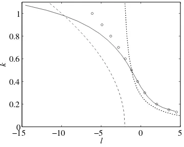
Figure 2. Neutral stability boundary in the (l, k)-plane forPr= 0.75,Q= 5 andθ= 70 (β= 9.72). Also shown are the infinite activation temperature results from Jackson & Kapila (1984) (open circles), the SVF results from Matalon & Matkowsky (1982) (dotted line) and the CDA results of Sivashinsky (1977) (dashed line).
These components then do not move away from zero in the correct direction, but in a way dictated by the numerical stepsize and starting value ofw. These incorrect values of the initially smaller components of u can then feedback and quickly pollute the numerical solution for all components ofu. However, provided one uses enough terms in the asymptotic expansions for the initial conditions of the numerical integration, such that the correct leading orderwdependency is retained for every component ofu, then the numerical solution follows the correct trajectory. Usually, this only involves retaining the first two or three terms in the asymptotic expansions. The only difficult case we have encountered using this method is for the stability of Chapman-Jouguet detonations, for which the singular point at the burnt boundary is an irregular singular point (Sharpe 1997b).
6. Results
In this section we compare our results with the asymptotic and numerical results of previous workers and examine the effect of each of the parameters on the stability of the steady, planar flame. The high activation temperature asymptotics show that the stability depends on the Lewis number through the parameter
l=β(1−1/Le),
0 0.1 0.2 0.3 0
0.02 0.04 0.06 0.08 0.1 0.12
k
[image:15.612.193.373.49.192.2]σ
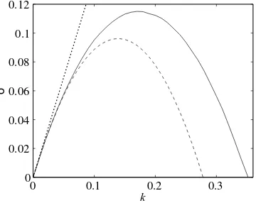
Figure 3. Dispersion relation for Pr = 0.75, Q = 5, Le = 1 and θ = 70 (β= 9.72). Also shown are the SVF (dashed line) and Landau-Darrieus (dotted line) dispersion relations.
6.1. Comparison with previous results
We first compare our exact linear dispersion relation results to those of high-activation temperature studies,β → ∞. Sivashinsky (1977) determined the dispersion relation for the CDA model, which is formally valid in the distinguished limitβ→ ∞,Q→0, to be
16σ3+ (48k2+ 8 + 2l−l2/4)σ2+ (1 + 12k2)(1 + 4k2+l/2)σ+
k2(1 + 4k2+l/2)2.
This gives a neutral stability boundary on whichσ = 0 given by
k= (−4−2l) 1 2
4
for l ≤ −2. Frankel & Sivashinsky (1982), Pelce & Clavin (1982) and Matalon & Matkowsky (1982) performed an SVF analysis, valid in the limitk→0 (i.e. valid for large wavelength disturbances) and determined the asymptotic expansion inkfor the dispersion relation, up toO(k2). Matalon & Matkowsky (1982) give this dispersion
relation in the form
σ =σ0k+σ1k2, (27)
where
σ0=
1 +Q
2 +Q "
1 +(2 +Q)Q 1 +Q
1 2
−1
# ,
σ1=
−(1 +Q)[lI(1 +σ0)(1 +Q+σ0) +Q
2+ (1 +Q) ln(1 +Q)(2(1 +σ
0) +Q)]
2Q[(1 +Q) + (2 +Q)σ0]
and
I =
Z 0
−∞
TheO(k) term in (27) is the Landau-Darrieus result. Jackson & Kapila (1984) then solved the leading order version of (17) in the limitβ → ∞numerically for arbitrary
Qandk.
Figure 2 shows the neutral stability boundary in the (l, k)-plane for Q = 5, Pr= 0.75 and a finite activation temperature ofθ= 70 (corresponding toβ = 9.72), together with the boundaries predicted from the CDA and SVF analyses as well as the infinite activation temperature results of Jackson & Kapila (1984). The flame is predicted to be stable to perturbations with wavenumbers above and to the left of the curves, and unstable for wavenumbers below and to the right of them. Note that our results and those of Jackson & Kapila (1984) show that the flame is always unstable to a band of wavenumbers between zero and the neutrally stable wavenumber. For Lewis numbers sufficiently close to or above unity (lclose to or above zero), the flame is only unstable to relatively small wavenumbers (large wavelengths). This is usually termed the ‘hydrodynamic’ instability. As the Lewis numbers decreases below unity (l negative), the flame becomes unstable to O(1) wavenumbers, i.e. to wavelengths comparable to the flame length. Here thermal-diffusive effects become important, and this is usually termed the ‘cellular’ instability. Note, however, that there is no clear distinction between the two regimes, the unstable band of wavenumbers continuously widens as Le decreases, and both hydrodynamic and thermal-diffusive (non-unity Lewis number) effects have a role in each regime.
Figure 2 shows that forl≥0 the results for finite activation temperature ofθ= 70 are in excellent quantitative agreement with the infinite activation temperature results of Jackson & Kapila (1984). However, forl <0, asldecreases and the flame becomes unstable to higher wavenumbers, the finite activation temperature results begin to diverge from those of Jackson & Kapila (1984).
β Le Q Pr σ σDH σF P
10 1 4 0.7 0.086 0.081
-10 0.9 4 0.7 0.145 0.143
-15 0.9333 4 0.7 0.142 0.140
-20 0.95 4 0.7 0.140 0.139
-10 0.9 2 0.71 0.074 - 0.077
10 0.9 4 0.71 0.145 - 0.14
10 0.9 8 0.71 0.260 - 0.26
[image:17.612.179.384.47.154.2]10 0.9 10 0.71 0.311 - 0.31
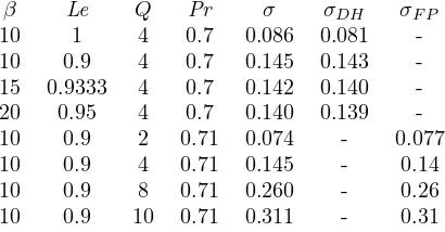
Table 1. Comparison of growth rates with those of Denet & Haldenwang (1995) and Fr¨olich & Peyret (1991) fork= 0.20944.
However, as discussed in§6.2, the infinite activation temperature results do not give good predictions for the instability at low Lewis numbers unlessβ is extremely large. Indeed, Lasseigne et al. (1999) found, using the CDA limit Q → 0 but with finite activation temperature, that the high activation temperature results of Sivashinsky (1977) do not give quantitatively good results for realistic values ofβ. Hence neither of the limitsQ→0 orβ→ ∞give accurate results for low Lewis number instabilities as compared to the results using realistic flame parameters. Of course, both asymptotic limits are useful for determining the qualitative trends and, more importantly, for revealing the physical mechanisms of the instability. Note that the stability boundary for finite activation temperature intersects with the high activation temperature CDA results (in this case at aboutl=−9). Hence asldecreases from zero, the CDA results initially underestimate the neutrally stable wavenumber, but for sufficiently large and negativel the CDA results overpredict this wavenumber.
It is also worth comparing our results with those of the finite activation temperature numerical simulations of Denet & Haldenwang (1995) and Fr¨olich & Peyret (1991), who both tabulated growth rates for various parameter sets for a wavenumber of 0.20944. Table 1 shows that the growth rates as measured from these non-linear simulations for the parameter sets given are in good agreement with the exact linear stability results. In the case of Denet & Haldenwang (1995) this includes the results for a relatively high Zeldovich number of β = 20. This attests to the careful implementation of the numerical method in Denet & Haldenwang (1995). The results of Fr¨olich & Peyret (1991) also compare well with the linear growth rates, which shows that their numerical scheme gives good results for relatively moderate activation temperatures (β= 10). However, in figure 3(d) of Fr¨olich & Peyret (1991) they show results forβ = 5,β = 10 andβ = 15 whenl=−1.11111. Their results forβ= 5 and
−25 −20 −15 −10 −5 0 5 0
0.2 0.4 0.6 0.8 1 1.2
l
k
(a)
0.5 1 1.5
0 0.2 0.4 0.6 0.8 1 1.2
Le
k
[image:18.612.99.459.50.192.2](b)
Figure 4. Neutral stability boundaries in (a) the (l, k)-plane and (b) the (Le, k )-plane, forPr = 0.75,Q= 4 and dotted lines: θ= 30 (β = 4.8), dashed lines:
θ= 50 (β= 8) and solid lines:θ= 70 (β= 11.2).
0 0.05 0.1 0.15 0.2
0 0.01 0.02 0.03 0.04 0.05
k
σ
(a)
0 0.5 1
0 0.2 0.4 0.6 0.8 1 1.2
k
σ
[image:18.612.101.458.245.387.2](b)
Figure 5. Dispersion relations for Pr = 0.75, Q = 4, (a) Le = 1.8 and (b)
Le= 0.3, and dotted lines: θ= 30 (β= 4.8), dashed lines: θ= 50 (β= 8) and solid lines: θ= 70 (β= 11.2).
6.2. Effect of activation temperature
We now explore the effect of the activation temperature in more detail. Figure 4 shows the neutrally stable wavenumber in (l, k)- and (Le, k)-planes, for Pr = 0.75,
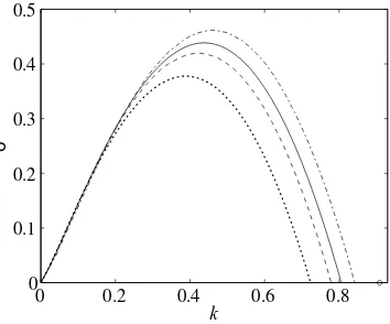
Q = 4 and activation temperatures of θ = 70 (corresponding to β = 11.2), θ = 50 (β = 8) and θ = 30 (β = 4.8). For Le = 1 (l = 0) we find that the stability is independent of the activation temperature. The curves in figure 4(b) all cross and meet atLe= 1. Figure 5 shows the dispersion relations whenLe= 1.8 andLe= 0.3 for various activation temperatures. Figures 4(b) and 5 also show that, for fixed Le > 1, increasing the activation temperature stabilizes the flame somewhat (the maximum growth rate decreases and the band of unstable wavenumbers narrows), while increasing activation temperature destabilizes the flame for fixed Le <1 (the maximum growth rate increases and the unstable band widens asθ increases).
0 0.2 0.4 0.6 0.8 0
0.1 0.2 0.3 0.4 0.5
k
[image:19.612.195.372.48.195.2]σ
Figure 6. Dispersion relations forPr= 0.75, Q= 4,l=−5 and dotted line:
θ= 30 (β= 4.8,Le= 0.4898), dashed line: θ= 50 (β= 8,Le= 0.6154), solid line: θ= 70 (β = 11.2,Le = 0.6914) and dot-dashed line θ= 140 (β = 22.4,
Le= 0.8175). Also shown as an open circle is the infinite activation temperature neutrally stable wavenumber.
(β = 4.8). Hence these results show that for the hydrodynamic instability, high activation temperature asymptotics give quantitatively good predictions even for not particularly high values of the activation temperature and even when the Lewis number isO(1) different from unity. This is also in agreement with the results of the numerical simulations of Denet & Haldenwang (1995), who found that the measured growth rates did not depend very much onβ for fixedl.
Forl <0, figure 4(a) shows that as l decreases, the neutral stability boundaries for different activation temperatures begin to rapidly diverge. Figure 6 shows the dispersion relations whenl=−5 forθ= 30, 50, 70 and 140 (corresponding toβ= 4.8, 8, 11.2 and 22.4, respectively). Note from figure 6 that at small wavenumbers, the growth rates are insensitive to the activation temperature, but that the dispersion relations for different activation temperatures diverge as the wavenumber increases. For comparison the neutrally stable wavenumber for infinite activation is also shown as the open circle. Even for a physically very large Zeldovich number of β = 22.4, the results are not well converged. The lower l, the slower the convergence to the infinite activation temperature results. Indeed, for low Lewis numbers the activation temperature must be very high for the infinite activation temperature results to give quantitatively good predictions. This sensitivity to the activation temperature for the cellular instability regime agrees with the finite activation temperature CDA results of Lasseigneet al. (1999) and the CDA numerical simulations of Denet & Haldenwang (1992), who both found that for the cellular instability the results for finite β were rather different from those forβ → ∞unless the activation temperature was extremely high.
6.3. Effect of heat release
Figure 7 shows the neutral stability boundary for Pr = 0.75, Q = 4 and θ = 70 (β = 11.2) as well as those when Q is increased to 8, with θ kept fixed (so that
−25 −20 −15 −10 −5 0 5 0
0.2 0.4 0.6 0.8 1 1.2
l
k
(a)
0.5 1 1.5
0 0.2 0.4 0.6 0.8 1 1.2
Le
k
[image:20.612.97.460.48.192.2](b)
Figure 7. Neutral stability boundaries in (a) the (l, k)-plane and (b) the (Le, k )-plane, forPr= 0.75 and dotted lines: Q= 8, θ= 70 (β= 6.91), dashed lines:
Q= 4,θ= 70 (β= 11.2) and solid line: Q= 8,θ= 113.4 (β= 11.2).
0 0.2 0.4 0.6 0.8 1
0 0.2 0.4 0.6 0.8
k
σ
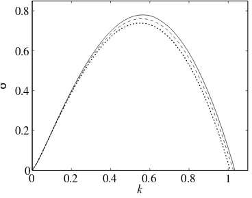
Figure 8. Dispersion relation forQ= 4,Le= 0.5,θ= 70 and Prandtl numbers 0.5 (dotted line), 0.75 (dashed line) and 1.0 (solid line).
neutral stability boundary forQ= 8 lies above and to the right of that forQ= 4). For fixed activation temperature,θ, the stability boundary forQ= 8 is in agreement with that for fixed β in the (l, k)-plane for l ≥0, and hence increasing Qdestabilizes the wave. However, the fixedθ and fixedβ boundaries diverge asl decreases below zero and the stability becomes sensitive to the activation temperature. At aboutl =−5 the neutral stability boundary forQ= 8 crosses that forQ= 4 whenθ is kept fixed, and hence forl <−5 increasingQstabilizes the flame.
6.4. Effect of viscosity
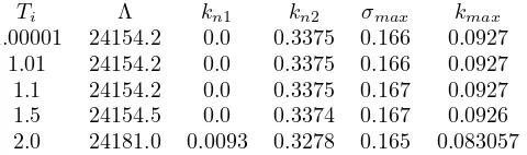
[image:20.612.190.374.247.392.2]Ti Λ kn1 kn2 σmax kmax
1.00001 24154.2 0.0 0.3375 0.166 0.0927
1.01 24154.2 0.0 0.3375 0.166 0.0927
1.1 24154.2 0.0 0.3375 0.167 0.0927
1.5 24154.5 0.0 0.3374 0.167 0.0926
[image:21.612.165.405.46.117.2]2.0 24181.0 0.0093 0.3278 0.165 0.083057
Table 2. Linear stability results forQ= 4,θ= 30 (β= 4.8),Pr= 0.75,Le= 1 and various ignition temperatures. Λ is the steady flame speed eigenvalue, kn1
andkn2are the neutrally stable wavenumbers,σmaxis the maximum growth rate
andkmaxthe corresponding wavenumber.
unity. However, it remains to check whether theO(1) wavenumber unstable cellular instability at lower Lewis numbers, for which the SVF analysis is not valid, is affected by viscosity. Note that in the CDA approximation, hydrodynamic effects are ignored and hence the CDA analysis cannot reveal anything about the effect of viscosity. Figure 8, which shows the dispersion relations forQ= 4,Le= 0.5,θ= 70 and various Prandtl numbers, reveals that for the cellular instability at lower Lewis numbers, viscosity has a slight destabilizing effect. Figure 8 shows that at low wavenumbers, the growth rates are very insensitive to the Prandtl number, in agreement with the SVF analysis. However, as the wavenumber increases and the SVF analysis becomes invalid, viscosity begins to play more of a role. At fixed higher wavenumbers, increasingPr increases the growth rates. Increasing the Prandtl number also increases the maximum growth rate and shifts the corresponding wavenumber to slightly higher values, and the band of unstable wavenumbers is also somewhat widened.
However, Addabbo, Bechtold & Matalon (2002) recently found that in the realistic case where the viscosity is allowed to vary with temperature, increasing Pr has a stabilizing effect on spherical flames. Hence in real flames, viscosity is likely to be stabilizing.
6.5. Effect of ignition temperature
As can be seen from figure 1(d), in the steady flame the reaction rate is exponentially small outside of a relatively thin reaction zone region. Indeed, for high activation temperature, the reaction rate is exponentially small whenever (1 +Q)−T0is larger
of the reaction zone, again resulting in a significant degree of reaction before the reaction zone is reached).
However, we should check that the stability results are also not sensitive to the ignition temperature. Table 2 shows the results for various ignition temperatures for a physically low Zeldovich number ofβ= 4.8 (for which the results will be most sensitive toTi). As can be seen both the steady flame solution (through the eigenvalue Λ) and the linear dispersion relation are very insensitive toTiprovidedTi is sufficiently close to one. Only whenTi−1 becomes O(1) does its value begin to have an effect. One point to note is that if too high a value of Ti is chosen (e.g. Ti = 2 in table 2), corresponding to the ignition point being inside the reaction zone, the lower neutrally stable wavenumber becomes positive and hencek= 0 becomes stable.
7. Conclusions
In this paper we have investigated the linear stability of freely propagating planar premixed flames for the Reactive Navier-Stokes equations with arbitrary values of the parameters, including finite activation temperature, using a numerical shooting method.
The exact linear stability results were compared to previous high activation temperature asymptotics. For Lewis numbers close enough to or above one, the finite activation temperature results agree with the infinite activation temperature results even for only moderate activation temperatures. Hence for these hydrodynamically dominated instabilities, the results are insensitive to the activation temperature for fixed l = β(1−1/Le). However, as the Lewis number decreases below unity and thermal-diffusive effects become important, the stability becomes more and more sensitive to the activation temperature, and the results for fixed finite activation temperature diverge from the infinite activation activation temperature results. At low Lewis numbers, very high activation temperatures are required for quantitative agreement with the asymptotic predictions. Slowly varying flame analyses, which are based on small wavenumber of the perturbation, give qualitatively good results, but underpredict the wavenumber with the maximum growth rate and the neutrally stable wavenumber. Neither of the limits assumed in the constant density approximation model of Sivashinsky (1977),β→ ∞andQ→0, give accurate results for the cellular instability when realistic values of the Zeldovich number and the heat release are used, and hence weakly nonlinear theories based on this model (Sivashinsky 1983) will also only give, at best, qualitative results.
The results were also compared with previous numerical simulations of the full non-linear problem, which demonstrated the role of exact linear stability analyses in validating numerical schemes for such simulations and determining in which parameter regimes a numerical method gives accurate results or fails.
A new result is that state-insensitive viscosity has a small destabilizing effect on the cellular instability at low Lewis numbers. However, in reality one must consider temperature dependent viscosity (Addabboet al. 2002).
and investigate the full non-linear evolution of unstable premixed flames, extending the results of Denet & Haldenwang (1995) and Kadowaki (1997, 1999, 2000), such as investigating the role of wall boundaries on unstable flames in tubes.
Acknowledgments
The author would like to thank Tom Jackson for providing the high activation temperature data from Jackson & Kapila (1984) and is grateful to Tom Jackson, Mark Short and John Buckmaster for useful discussions and encouragement at the start of this work.
References
Addabbo, R., Bechtold, J.K. & Matalon, M.2002 Wrinkling of spherically expanding flames.
29th Symposium (International) on Combustion, to appear.
Bourlioux, A., Majda, A. J. & Roytburd, V. 1991 Theoretical and numerical structure for
unstable one-dimensional detonations.SIAM J. Appl. Math.51, 303–343.
Buckmaster, J. D.1983 Stability of porous plug burner flame.SIAM J. Appl. Math.431335–1349.
Buckmaster, J. D. & Ludford, G. S. S.1982Theory of Laminar Flames.Cambridge University
Press.
Bush, W. B. & Fendell, E. F.1970 Asymptotic analysis of laminar flame propagation for general
Lewis numbers.Combust. Science Tech.1421–428.
Denet, B. & Haldenwang, P.1992 Numerical study of thermal-diffusive instability of premixed
flames.Combust. Science Tech.86199–221.
Denet, B. & Haldenwang, P. 1995 A numerical study of premixed flames Darrieus-Landau
instability.Combust. Science Tech.104143–167.
Dold, J., Weber, R. O., Thatcher, R. W. & Shah, A. A.2002 Flame ball with thermally sensitive
intermediate kinetics.Combust. Theory Model., submitted.
Frankel, M. L. & Sivashinsky, G. I.1982 The effect of viscosity on hydrodynamic stability of a
plane flame front.Combust. Science Tech.29, 207–224.
Fr¨olich, J. & Peyret, R. 1991 A spectral algorithm for low Mach number combustion. Comp.
Meth. App. Mech. Eng.90, 631–642.
Gasser, I. & Szmolyan, P. 1993 A geometric singular perturbation analysis of detonation and
deflagration waves.SIAM J. Math. Anal.24, 968–986.
Gasser, I. & Szmolyan, P.1995 Detonation and deflagration waves with multistep reaction schemes.
SIAM J. Appl. Math.55, 175–191.
Gubernov, V., Mercer, G. N., Sidhu, H. S. & Weber, R. O.2001 Numerical methods for the
travelling wave solutions in reaction-diffusion frontsANZIAM J., to appear.
Jackson, T. L. & Kapila, A. K.1984 Effect of thermal expansion on the stability of plane, freely
propagating flame.Combust. Science Tech.41, 191–201.
Jackson, T. L. & Kapila, A. K.1986 Thermal expansion effects on perturbed premixed flames: a
review.Lectures in App. Math.24, 325–347.
Joulin, G. & Clavin, P.1979 Linear stability analysis of nonadiabatic flames: diffusional-thermal
model.Combust. Flame 35, 139–153.
Kadowaki, S.1997 Numerical study of lateral movements of cellular flames.Phys. Rev.E56, 2966–
2971.
Kadowaki, S.1999 The influence of hydrodynamic instability on the structure of cellular flames.
Phys. Fluids11, 3426–3433.
Kadowaki, S. 2000 Numerical study on the formation of cellular premixed flames at high Lewis
numbers.Phys. Fluids 12, 2352–2359.
Landau, L. D. & Lifshitz, E. M.1959Fluid Mechanics.Pergamon.
Lasseigne, D. S., Jackson, T. L. & Jameson, L.1999 Stability of freely propagating flames revisited.
Combust. Theory Model.,3, 591-611.
Liberman, M. A., Bychkov, V. V., Goldberg, S. M. & Book, D. L.1994 Stability of a planar
flame front in the slow-combustion regime.Physical Review E,49, 445–453.
Matalon, M. & Matkowsky, B. J.1982 Flames as gasdynamic discontinuities.J. Fluid Mech.124,
Mukunda, H. S. & Drummond, J. P.1993 Two dimensional linear stability of premixed laminar flames under zero gravity.Appl. Scientific Research51, 687–711.
Ng, B. S. & Reid, W. H.1985 The compound matrix method for ordinary differential systems.J.
Comp. Phys.58, 209–228.
Pelce, P. & Clavin, P.1982 Influence of hydrodynamics and diffusion upon the stability limits of
laminar premixed flames.J. Fluid Mech.124, 219–237.
Rogg, B.1982 The effect of Lewis number greater than unity on an unsteady propagating flame with
one-step chemistry. InNumerical Methods in Laminar Flame Propagation (ed. N. Peters & J. Warnatz), pp 38–48. Vieweg.
Shah, A. A., Thatcher, R. W. & Dold, J. W.2000 Stability of a spherical flame ball in a porous
medium.Combust. Theory Model.4, 511–534.
Sharpe, G. J.1997aLinear stability of idealized detonations.Proc. Roy. Soc. Lond.A453, 2603–
2625.
Sharpe, G. J.1997bDetonation waves in type I supernovae. PhD thesis, University of Leeds.
Sharpe, G. J.1999 Linear stability of pathological detonations.J. Fluid Mech.401, 311–338.
Sharpe, G. J. & Falle, S. A. E. G. 2000a Numerical simulations of pulsating detonation: I.
Nonlinear stability of steady detonations.Combust. Theory Model.4, 557-574.
Sharpe, G. J. & Falle, S. A. E. G. 2000b Two-dimensional numerical simulations of idealized
detonations.Proc. Roy. Soc. Lond.A456, 2081-2100.
Short, M. & Quirk, J. J.1997 On the nonlinear stability and detonability limit of a detonation
wave for a model three-step chain-branching reaction.J. Fluid Mech.339, 89-119.
Short, M., Buckmaster, J. & Kochevets, S.2001 Edge-flames and sublimit hydrogen combustion.
Combust. Flame125, 893-905.
Singh, G. & Clarke, J. F.1992 Transient phenomena in the initiation of a mechanically driven
plane detonationProc. Roy. Soc. Lond.A438, 23–46.
Sivashinsky, G. I.1977 Diffusional-thermal theory of cellular flames Combust. Sci. Tech.15, 137–
146.
Sivashinsky, G. I.1983 Instabilities, pattern formation, and turbulence in flames.Ann. Rev. Fluid
Mech.15, 179–199.
Strehlow, R. A.1985Combustion Fundamentals.McGraw-Hill.
Williams, F. A.1985Combustion Theory, 2nd Ed. Addison-Wesley Publishing.
Zeldovich, Y. B., Barenblatt, G. I., Librovich, V. B. & Makhviladze, G. M. 1985 The
Mathematical Theory of Combustion and Explosions, Plenum Publishing.
Zhang, Z. & Falle, S. A. E. G.1994 Stability of reaction-diffusion fronts.Proc. R. Soc. Lond.A