The definition of the relevant population and the collection of data for likelihood ratio-based forensic voice comparison

(1)

population and the collection of data

for likelihood ratio-based forensic

voice comparison

Vincent Stephen Hughes

PhD

University of York

Language and Linguistic Science

(2)

(3)

Within the field of forensic speech science there is increasing acceptance of the

likeli-hood ratio (LR) as the logically and legally correct framework for evaluating forensic

voice comparison (FVC) evidence. However, only a small proportion of experts

cur-rently use the numerical LR in casework. This is due primarily to the difficulties

involved in accounting for the inherent, and arguably unique, complexity of speech in a

fully data-driven, numerical LR analysis. This thesis addresses two such issues: the

definition of the relevant population and the amount of data required for system testing.

Firstly, experiments are presented which explore the extent to which LRs are affected

by different definitions of the relevant population with regard to sources of systematic

sociolinguistic between-speaker variation (regional background, socio-economic class

and age) using both linguistic-phonetic and ASR variables. Results show that different

definitions of the relevant population can have a substantial effect on the magnitude

of LRs, depending on the input variable. However, system validity results suggest

that narrow controls over sociolinguistic sources of variation should be preferred to

general controls. Secondly, experiments are presented which evaluate the effects of

development, test and reference sample size on LRs. Consistent with general principles

in statistics, more precise results are found using more data across all experiments.

There is also considerable evidence of a relationship between sample size sensitivity

and the dimensionality and speaker discriminatory power of the input variable. Further,

there are potential trade-offs in the size of each set depending on which element of LR

output the analyst is interested in. The results in this thesis will contribute towards

im-proving the extent to which LR methods account for the linguistic-phonetic complexity

of speech evidence. In accounting for this complexity, this work will also increase the

(4)

Abstract i

Contents ii

List of Tables ix

List of Figures xi

Acknowledgements xx

Declaration xxii

1 Introduction 1

1.1 Forensic voice comparison . . . 2

1.1.1 Auditory phonetic analysis . . . 3

1.1.2 Acoustic phonetic analysis . . . 3

1.1.3 Combined auditory and acoustic analysis . . . 4

1.1.4 Automatic speaker recognition (ASR) . . . 5

1.2 Expressing conclusions in forensic science . . . 6

1.3 Research aims and implications . . . 7

1.4 Overview of the thesis . . . 9

2 Research Review 11 2.1 Conclusion frameworks in FVC . . . 13

2.1.1 Binary decision . . . 13

2.1.2 Classical probability scales . . . 14

(5)

2.1.3.1 Limitations of UKPS . . . 18

2.1.4 The Bayesian approach . . . 18

2.1.4.1 Bayes’ theorem and Bayesian reasoning . . . 19

2.1.4.2 Assessing strength of evidence using the LR . . . . 21

2.1.4.3 Logical and legal correctness of the LR . . . 23

2.1.4.4 Logical fallacies . . . 24

2.1.4.5 Bayes and the LR in the courts . . . 25

2.2 The LR in FVC . . . 26

2.2.1 Acceptance of the LR framework for FVC . . . 26

2.2.2 LR-based research . . . 27

2.2.3 LR-based casework . . . 29

2.2.4 Issues with the LR in FVC . . . 32

2.2.5 Complexity of speech evidence . . . 34

2.3 Definition of the relevant population . . . 36

2.3.1 Logical relevance . . . 38

2.3.1.1 Limitations . . . 39

2.3.2 Lay listener-judged similarity . . . 41

2.3.2.1 Limitations . . . 43

2.4 Collection of development, test and reference data . . . 45

2.4.1 Going and getting it(Rose 2007b) . . . 46

2.4.2 Off-the-shelf data . . . 47

2.4.2.1 General corpora . . . 47

2.4.2.2 Forensic databases . . . 48

2.5 Amount of development, test and reference data . . . 48

2.6 Research questions . . . 53

3 General Methodology 55 3.1 Corpora . . . 55

3.1.1 Dynamic Variability in Speech (DyViS) . . . 55

3.1.2 Origins of New Zealand English (ONZE) . . . 57

3.1.3 Northern Englishes (NE) . . . 58

(6)

3.2 LR testing . . . 60

3.2.1 Development, test and reference data . . . 61

3.2.2 Feature-to-score stage . . . 62

3.2.2.1 Modelling . . . 62

3.2.2.2 Intrinsic vs. extrinsic testing . . . 67

3.2.2.3 Independent sets vs. cross-validation . . . 67

3.2.2.4 Log likelihood ratios (LLRs) . . . 68

3.2.2.5 Tippett plots . . . 69

3.2.2.6 Verbal LRs . . . 70

3.2.3 System performance: validity and reliability . . . 71

3.2.3.1 Validity . . . 71

3.2.3.2 Reliability . . . 74

3.2.4 Score-to-LR mapping . . . 75

3.2.4.1 Logistic regression calibration . . . 75

3.3 Input variables . . . 77

3.3.1 Formant dynamics . . . 78

3.3.1.1 Speaker discrimination and individual formants . . 79

3.3.1.2 Data extraction . . . 82

3.3.1.3 Defining the onset and offset of vowel tokens . . . . 83

3.3.1.4 Parametric representations of formant trajectories . 85 3.3.2 Cepstral coefficients and derivatives . . . 91

3.3.2.1 Extracting cepstral coefficients and derivatives . . . 92

3.4 Limitations . . . 95

4 Regional Background: /u:/ 97 4.1 Introduction . . . 97

4.2 Method . . . 98

4.2.1 Data . . . 98

4.2.2 Variation and change in /u:/ . . . 99

4.2.3 Dynamic formant extraction . . . 100

4.2.4 Variability in the data . . . 102

(7)

4.3.1 Experiment (1): Multiple test sets . . . 105

4.3.2 Experiment (2): Multiple systems . . . 109

4.4 Discussion . . . 111

4.5 Chapter summary . . . 113

5 Regional Background: /aI/ 114 5.1 Introduction . . . 114

5.2 Method . . . 116

5.2.1 Data . . . 116

5.2.2 Variation and change in /aI/ . . . 117

5.2.3 Dynamic formant extraction . . . 118

5.2.5 Experiments . . . 121

5.3 Results . . . 123

5.3.1 Experiment (1): Multiple systems . . . 123

5.3.2 Experiment (2): Regional patterns . . . 128

5.3.3 Experiment (3): Speaker-specific patterns . . . 130

6 Regional Background: Cepstral Coefficients and Derivatives 136 6.1 Introduction . . . 136

6.2 Method . . . 140

6.2.1 Data . . . 140

6.2.2 Preparation of samples . . . 141

6.2.3 Linguistic differences between dialect regions . . . 143

6.2.4 Feature extraction . . . 147

6.2.5 Experiment . . . 148

6.3 Results . . . 150

6.3.1 Mel Frequency cepstrum . . . 150

6.3.1.1 Reliability . . . 155

(8)

7 Socio-Economic Class and Age: /eI/ 166 7.1 Introduction . . . 166

7.2 Method . . . 167

7.2.1 /eI/ in New Zealand English . . . 167

7.2.2 Data . . . 168

7.2.3 Dividing the data . . . 169

7.2.4 Parametric representations . . . 171

7.2.5.1 Socio-economic class . . . 173

7.2.5.2 Age . . . 174

7.2.5.3 Interaction between class and age . . . 176

7.2.6 Experiment . . . 177

7.3 Results . . . 180

7.3.1 Socio-economic class . . . 180

7.3.2 Age . . . 182

7.3.3 Reliability . . . 184

7.3.4 Systematic patterns or random variation? . . . 185

8 Reference Sample Size: Raw Data 193 8.1 Introduction . . . 193

8.2 Method . . . 195

8.2.1 Data . . . 195

8.2.1.1 /u:/ . . . 195

8.2.1.2 /aI/ . . . 195

8.3 Results . . . 197

(9)

8.3.1.2 /aI/ . . . 200

8.3.2 Experiment (2): Number of tokens per reference speaker . . . 204

8.3.2.1 /u:/ . . . 204

8.3.2.2 /aI/ . . . 207

9 Reference Sample Size: Univariate Monte Carlo Simulations 215 9.1 Introduction . . . 215

9.2 Method . . . 217

9.2.1 Data . . . 217

9.2.2 Modelling . . . 218

9.2.3 Monte Carlo simulations . . . 221

9.2.3.1 Synthetic means . . . 221

9.2.3.2 Synthetic SDs . . . 223

9.2.3.3 Synthetic data . . . 225

9.3 Results . . . 228

9.3.1 Experiment (1): Number of reference speakers . . . 228

9.3.2 Experiment (2): Number of tokens per reference speaker . . . 232

10 Development, Test and Reference Sample Size: Multivariate Monte Carlo Simulations 240 10.1 Introduction . . . 240

10.2 Method . . . 242

10.2.1 Choice of variable . . . 242

10.2.2 Data . . . 244

10.2.2.1 Formant correction . . . 245

10.2.2.2 Mid-points vs. dynamics . . . 245

(10)

10.2.3.2 Correlations . . . 252

10.2.4 Monte Carlo simulations . . . 253

10.2.5 Experiments . . . 255

10.3 Results . . . 258

10.3.1 Experiment (1): Number of development speakers . . . 258

10.3.2 Experiment (2): Number of test speakers . . . 262

10.3.3 Experiment (3): Number of reference speakers . . . 265

11 Discussion and Conclusions 276 11.1 Defining the relevant population . . . 276

11.1.1 Emulating DNA . . . 285

11.1.1.1 Multiple defence propositions . . . 285

11.1.1.2 Correction factor (F) . . . 286

11.1.2 Emulating ASR . . . 287

11.1.2.1 Expert-judged speaker similarity . . . 287

11.2 Collecting development, test and reference data . . . 290

11.3 Practical implications . . . 292

11.4 Future work . . . 295

11.5 Conclusion . . . 298

Appendix 300

List of abbreviations 302

Legal Cases 305

(11)

2.1 Example of a classical probability scale for FVC conclusions

(Broed-ers 1999: 129; equivalent to that in Baldwin and French 1990: 10) . . 14

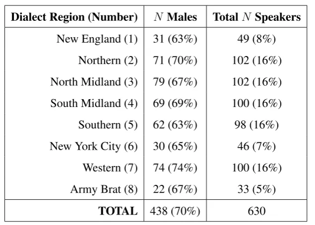
3.1 Number of male speakers in each of the dialect regions (DRs) in the

TIMIT corpus (from Garofoloet al.1993: 16) . . . 61

3.2 Raw values with base 10 and base e logarithm values . . . 69

3.3 Verbal expressions of raw and LLRs according to Champod and Evett’s

(2000: 240) scale . . . 71

3.4 Categoricalcorrect(consistent-with-fact) andincorrect

(contrary-to-fact) decisions made by a LR-based biometric system (equivalent to

that in Morrison 2011b: 93) . . . 72

3.5 Criteria used to define the onset of vowel tokens based on the preceding

sound . . . 84

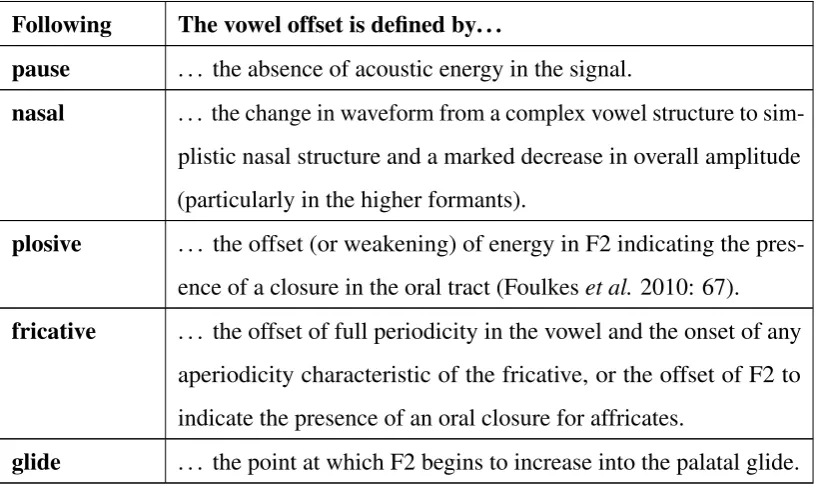
3.6 Criteria used to define the offset of vowel tokens based on the following

sound . . . 85

3.7 Target items containing /aI/ elicited by the interviewer for DyViS . . . 88

4.1 Phonological categorisation of /u:/ tokens and the maximum number of

tokens in such contexts shared by every test speaker . . . 101

4.2 Percentage of tokens in each of the four phonological contexts for the

NZ test and reference sets . . . 101

4.3 EER andC_llrusing Matched and Mixed data in both the feature-to-score

and score-to-LR stages . . . 111

5.1 Cross-validated classification rates of tokens correctly assigned to

(12)

gional set based on DA using individual cubic coefficients from F1, F2

and F3 . . . 130

6.1 Number of development, test and reference speakers used in each

system within each experiment . . . 144

6.2 Transcription conventions used by Labovet al. (1997) with the

equiva-lent lexical set (Wells 1982) and IPA phonemic transcription . . . 146

6.3 Mean 95% CIs (±LLR) for CCs and derivatives and CCs-only from the MFC and the LPC . . . 163

6.4 Ranges of EER (%) and C_llr values across all systems for CCs and

derivatives and CCs-only from the MFC and the LPC . . . 164

7.1 Number of development, test and reference speakers used in each

system within each experiment . . . 178

9.1 Mean and SD of mean local AR (syllables/ s) for the raw data, synthetic

data and all reference data . . . 225

9.2 Mean and SD of SD local AR (syllables/ s) for the raw data, synthetic

data and all reference data . . . 225

10.1 Number of available speakers and tokens per speaker (maximum,

mini-mum and mean) for each of the variable . . . 243

10.2 C_llrand EER performance for each variable . . . 244

10.3 z-scores for skew and kurtosis based on the raw means and SDs for F1, F2 and F3 (with significant values highlighted in red (p< 0.01) and orange (p< 0.05)) . . . 248 10.4 z-scores for skew and kurtosis based on the log SDs for F1, F2 and F3 249 10.5 Partial correlation matrix based on pairwise Pearson correlation test

withrho(left) and p-values (right, italics) for F1, F2 and F3 means and SDs for UM based on input data form 86 speakers (significant

(13)

2.1 Flow chart of the UK Position Statement framework for FVC evidence

(from Rose and Morrison 2009: 143) . . . 16

2.2 Univariate example of a LR computed using Lindley’s (1977) model

for a same speaker comparison based on midpoint F1 (Hz) values for

New Zealand English (NZE) /u:/ . . . 22

3.1 Example of a slide from DyViS Task 1 containing information about

the mock suspect’s story (Nolanet al.2009: 42) . . . 56

3.2 Map of USA with TIMIT dialect regions marked (from Garofoloet al.

1993: 17) . . . 60

3.3 Bivariate example of a MVKD LR computed for a same speaker

com-parison based on midpoint F1 and F2 (Hz) values using data from

ONZE . . . 64

3.4 GMMs of hypothetical suspect and reference data for f0 constructed

using four Gaussians per model (from Morrison 2010: 28) . . . 66

3.5 Tippett plot based on hypothetical SS and DS LRs produced by a FVC

system . . . 70

3.6 Visual representation of validity (accuracy) and reliability (precision)

(from Morrison 2011b: 92) . . . 72

3.7 Visual representation of logistic regression calibration involving

mod-elling of SS (red) and DS (blue) scores for a set of development data

with Gaussian curves (panel 1), with a probability curve (panel 2) and

the linear relationship between the score and the LLR in the log-odds

(14)

measurements taken at +10% steps (McDougall 2004) for a token of

/aI/ from the wordskypefrom DyViS sample 027-1-060425.wav . . . 82

3.9 Raw F2 (Hz) trajectory for a token of /aI/ from the wordskype from

DyViS sample 027-1-060425.wav (as in Figure 3.8) fitted with quadratic,

cubic and quartic polynomial curves . . . 87

3.10 Tippett plot of SS (solid) and DS (dashed) LLRs using quadratic

(or-ange), cubic (green) and quartic (purple) representations of the F1∼F3 trajectories of /aI/ . . . 89

3.11 C_llrplotted against EER using quadratic (orange), cubic (green) and

quartic (purple) input . . . 90

3.12 Visual representation of extraction of cepstral (in this case MFC)

infor-mation from a speech signal (Jurafsky 2007) . . . 93

3.13 Relationship between linear and Mel frequency scales . . . 94

3.14 Graphical representation of the Mel (above) and linear frequency

(be-low) filterbank applied to the power spectrum from a given window,

with 50% overlap between filters (from Lei and Lopez-Gonzalo 2009:

2324) . . . 95

4.1 F1∼F2 plots of individual tokens of /u:/ (post-/j/ and in open syllables) at the +50% step (mid-point) of formant trajectories for each of the test

speakers . . . 103

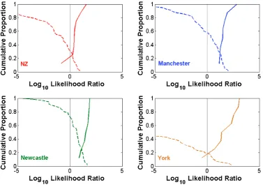
4.2 Tippett plots of SS and DS scores based on F1 and F2 trajectories from

/u:/ for the NZ (top left) (Matched), Manchester (top right), Newcastle

(bottom left) and York (bottom right) (Mismatched) test sets . . . 106

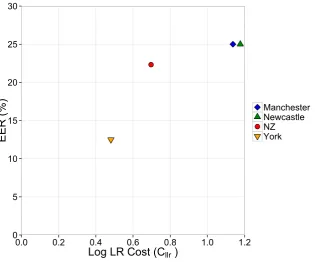
4.3 C_llrplotted against EER (%) for each of the test sets based on F1 and

F2 from /u:/ . . . 107

4.4 Tippett plots of SS and DS scores based on F2-only trajectories from

/u:/ for the NZ (top left) (Matched), Manchester (top right), Newcastle

(bottom left) and York (bottom right) (Mismatched) test sets . . . 108

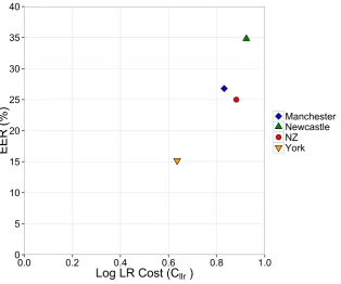
4.5 C_llrplotted against EER (%) for each of the test sets based on F2-only

(15)

Matched (red) and Mixed (green) data in both the feature-to-score and

score-to-LR stages . . . 110

5.1 Dialect map of the British Isles with isoglosses marking regional

vari-ants of /aI/ (from Upton and Widdowson 2006: 32) . . . 117

5.2 F1∼F2 plot of mean /aI/ trajectories for DyViS (red), Derby (orange), Manchester (blue) and Newcastle (green) (eight speakers per set, ten

to-kens per speaker) with mean mid-point values for FLEECE /i:/, GOOSE

/u:/, NORTH /O:/ and TRAP /a/ (based on the first 20 DyViS speakers) 120

5.3 Mean F1∼F3 trajectories for each speaker by regional set (based on ten tokens per speaker) . . . 121

5.4 Tippett plot of SS and DS LLRs based on F1∼F3 trajectories from /aI/ using Matched (red) and Mixed (green) system data . . . 124

5.5 Tippett plot of SS and DS LLRs based on F2 and F3 trajectories from

/aI/ using Matched (red) and Mixed (green) system data . . . 125

5.6 Tippett plot of SS and DS LLRs based on F3-only trajectories from /aI/

using Matched (red) and Mixed (green) system data . . . 126

5.7 EER (%) based on F1∼F3, F2 and F3, and F3-only input from /aI/ using Matched (red) and Mixed (green) system data . . . 127

5.8 Log LR Cost (Cllr) based on F1∼F3, F2 and F3, and F3-only input

from /aI/ using Matched (red) and Mixed (green) system data . . . 128

5.9 Tippett plot of SS and DS LLRs using F1-only (blue), F2-only (red),

F3-only (green) and a combination of the three formants (orange) of

/aI/ from DyViS . . . 131

5.10 Log LR Cost (Cllr) plotted against EER (%) for different DyViS formant

input for /aI/ . . . 132

6.1 RMS amplitude analysis using the Sound File Cutter Upper software

for speaker MCEW0 007 from DR 2 with the default threshold between

(16)

identified through analysis of 240 participants (marked as points on the

map) as part of the Telsur project (Labovet al. 1997) . . . 143

6.3 Map of the North Central, Inland North, New England, New York,

Midland and South dialect areas as identified by Labovet al.(1997) . 145

6.4 Phonological taxonomyof vocalic differences between the major dialect

regions of North American English (Labovet al. 1997) . . . 147

6.5 Boxplots (mid line = median, filled box = interquartile range (containing

middle 50% of the data), whiskers = scores outside the middle 50%,

dots = outliers) of SS (above) and DS (below) LLRs for each system

using CCs and derivatives from the MFC . . . 151

6.6 C_llrplotted against EER (%) for each system using CCs and derivatives

from the MFC . . . 152

6.7 Box plots of SS (above) and DS (below) LLRs for each system using

CCs-only from the MFC . . . 153

6.8 C_llrplotted against EER (%) for each system using CCs-only from the

MFC . . . 154

6.9 Tippett plots of mean SS (light) and DS (dark) LLRs and 95% CIs

across systems using CCs and derivatives (left; red) and CCs-only

(right; blue) from the MFC . . . 155

6.10 Boxplots of SS (above) and DS (below) LLRs for each system using

CCs and derivatives from the LPC . . . 157

6.11 C_llrplotted against EER (%) for each system using CCs and derivatives

from the LPC . . . 158

6.12 Boxplots of SS (above) and DS (below) LLRs for each system using

CCs-only from the LPC . . . 159

6.13 C_llrplotted against EER (%) for each system using CCs-only from the

LPC . . . 160

across systems using CCs and derivatives (left; red) and CCs-only

(17)

cultivated (above) and broad(below) NZE (adapted from Hay et al.

2008: 97) . . . 168

7.2 Density plot of bimodal distribution of year of birth from the entire

dataset (solid) and from the subdivided dataset consisting of speakers

born before 1950 and after 1970 (dashed) . . . 170

7.3 Raw F3 values (y) for a single token fitted with a cubic polynomial (y-fit) (red dashed curve) (above) and values with a residual greater than±100 Hz identified (dashed ellipsis) (below) . . . 172 7.4 Mean F1, F2 and F3 trajectories with 95% CIs plotted by class based

on 120 male speakers and eight tokens per speaker . . . 174

7.5 Mean F1, F2 and F3 trajectories with 95% CIs plotted by age based on

120 male speakers and eight tokens per speaker . . . 175

7.6 F1∼F2 plot of mean /eI/ trajectories according to age and class for 120 speakers based on eight tokens per speaker . . . 177

7.7 Tippett plot of SS and DS LLRs using the three class-based systems . 180

7.8 C_llrplotted against EER (%) for each of the three class-based systems 181

7.9 Tippett plot of SS and DS LLRs using the three age-based systems . . 183

7.10 C_llrplotted against EER (%) for each of the three age-based systems . 184

across the three systems based on class (left; red) and age (right; blue) 185

7.12 Boxplots of median SS and DS LLRs for the three class-based systems

across the 20 replications . . . 186

7.13 Boxplots of the distributions EER (left) andCllr(right) values for the

three class-based systems across the 20 replications . . . 187

7.14 Boxplots of median SS and DS LLRs for the three age-based systems

across the 20 replications . . . 188

7.15 Boxplots of the distributions EER (left) andCllr(right) values for the

(18)

middle 50% of the data), whiskers = scores outside the middle 50%,

dots = outliers; following Rose 2012) of SS scores based on /u:/ as a

function of the number of reference speakers with they-axis scaled to between +5 and -5 (outliers with ten speakers extent to -16) . . . 197

8.2 Boxplots of DS scores based on /u:/ as a function of the number of

reference speakers with they-axis scaled to between +2 and -10 (for allN speakers outliers extend to -20, with outliers using 10 speakers extending to almost -40) . . . 198

8.3 EER (%) based on /u:/ as a function of the number of reference speakers199

8.4 C_llrbased on /u:/ as a function of the number of reference speakers in

all conditions (left) and with between 20 and 120 speakers with linear

trend (right) . . . 200

8.5 Boxplots of SS scores based on /aI/ as a function of the number of

reference speakers with they-axis scaled to between 10 and -5 (outliers with 10 speakers extent from c. +13 to -21) . . . 201

8.6 Boxplots of DS scores based on /aI/ as a function of the number of

ref-erence speakers with they-axis scaled to between +5 and -20 (outliers with ten speakers extent from c. +10 to -80) . . . 202

8.7 EER (%) based on /aI/ as a function of the number of reference speakers203

8.8 C_llrbased on /aI/ as a function of the number of reference speakers in

all conditions (left) and with between 20 and 89 speakers (right) . . . 204

8.9 Boxplots of SS scores based on /u:/ as a function of the number of

tokens per reference speaker with they-axis scaled to between +3 and -1 (outliers extend to c. -10 using two tokens per reference speaker) . . 205

8.10 Boxplots of DS scores based on /u:/ as a function of the number of

tokens per reference speaker with they-axis scaled to between +2 and -10 (outliers across all conditions extend to > -10, with outliers of up to

-30 using two tokens per speaker) . . . 205

8.11 EER (%) based on /u:/ as a function of the number of tokens per

(19)

speaker . . . 207

8.13 Boxplots of SS scores based on /aI/ as a function of the number of

reference speakers with they-axis scaled to between 10 and -5 (outliers with 10 tokens per speaker extent from c. +13 to -21) . . . 208

8.14 Boxplots of DS scores based on /aI/ as a function of the number of

ref-erence speakers with they-axis scaled to between +5 and -20 (outliers with two tokens per speaker extent from c. +167 to -136) . . . 208

8.15 EER (%) based on /aI/ as a function of the number of tokens per

reference speaker . . . 209

8.16 C_llrbased on /aI/ as a function of the number of tokens per reference

speaker . . . 210

9.1 Histograms of AR means (left) and SDs (right) for each of the 59 raw

speakers fitted with normal distributions . . . 219

9.2 p-values based on t-tests comparing the distributions of means (left) and SDs (right) for the number of speakers on thex-axis against that with all 59 raw speakers with 1% (red) and 5% (orange) significance

marked . . . 220

9.3 Example of the inverse CDF of mean local AR used to generate a syntheticzi of 0 based on a random Zi of 0.5 (zi = 0 equates toxi =

6.044; i.e. the mean of the raw data) . . . 222

9.4 Mean local AR plotted against SD of local AR (syllables/ s) for each of

the 59 raw speakers . . . 224

9.5 Mean local AR values (syllables/ s) plotted against SD of local AR

(syllables/ s) for the 59 speakers from the raw data (left) and the 941

synthetic speakers (right) with linear trend lines fitted . . . 226

9.6 Boxplots of SS (above) and DS (below) LLRs as a function of the

number of reference speakers . . . 229

9.7 EER (%) (left) andC_llr(right) as a function of the number of reference

speakers with the truevalue (based on 1000 speakers plotted with a

(20)

number of reference speakers . . . 231

9.9 Boxplots of SS (above) and DS (below) LLRs as a function of the

number of tokens per reference speaker . . . 233

9.10 EER (%) (left) andC_llr(right) as a function of the number of reference

speakers with the true value (based on 100 speakers plotted with a

dashed maroon line) . . . 234

9.11 Boxplots of SS (above) and DS (below) scores as a function of the

number of tokens per reference speaker . . . 235

10.1 Example of a segmented token of UM on a PRAAT TextGrid from

DyViS speaker 58 . . . 245

10.2 Histograms of raw means (left) and SDs (right) for F1 (red), F2 (blue)

and F3 (green) based on 86 speakers fitted with a kernel density . . . 247

10.3 Histograms of the natural logarithms of raw SDs for F1 (red), F2 (blue)

and F3 (green) based on 86 speakers fitted with a kernel density . . . 250

10.4 Means (solid) and 95% CIs (dashed) for F1 (red), F2 (blue) and F3

(green) means (left) and logged SDs (right) based on the number of

speakers included . . . 251

10.5 Scatterplots of F1 SDs and F2 SDs fitted with a linear trend line and

using data from all 86 speakers (left; the outlying speaker is marked

with a red ellipse) and with the outlying speaker removed (right) . . . 253

10.6 CDFs of F1 (red), F2 (blue) and F3 (green) means (left) and SDs (right) based on the raw data (86 speakers) and an example set of 1000

synthetic speakers . . . 255

10.7 Mean (blue) and 95% CIs (grey) of calibration scale values as a function

of the number of development speakers (left = two to 1000 speakers,

right = two to 50 speakers) . . . 259

10.8 Mean (purple) and 95% CIs (grey) of calibration shift values as a

function of the number of development speakers (left = two to 1000,

right = three to 50) . . . 260

10.9 Scatterplot of median SS LLRs using between two and 100 development

(21)

ment speakers fitted with mean (blue) and 95% CIs (grey) (outliers

extend from +1.94 to -90.64 using two development speakers) . . . . 261

10.11Scatterplot ofC_llrvalues (left; scale = 0-3) using between two and 100

development speakers fitted with mean and 95% CIs (right; scale = 0-1) 262

10.12Scatterplot of median SS LLRs using between two and 100 test speakers

fitted with mean (red) and 95% CIs (grey) . . . 263

10.13Boxplots of median DS LLRs as a function of the number of test speakers264

10.14Scatterplot of EER (left) andC_llr(right) as a function of the number of

test speakers fitted with the group mean and 95% CIs (grey) . . . 265

10.15Mean and 95% CIs of calibration shift (left) and scale (right) values

using between 10 and 100 reference speakers . . . 266

10.16Boxplots of median calibrated SS (above) and DS (below) LLRs as a

function of the number of reference speakers . . . 267

10.17Scatterplot of EER (left) andC_llr(right) based on LLRs as a function of

the number of reference speakers fitted with the group mean and 95% CIs268

10.18Boxplots of median SS (above) and DS (below) scores as a function of

the number of reference speakers . . . 270

10.19Scatterplot of C_llr based on scores as a function of the number of

reference speakers fitted with the group mean and 95% CIs . . . 271

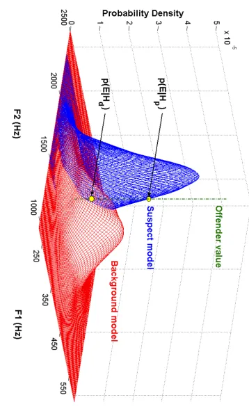
11.1 Univariate example of a SS comparison (test speaker 11) from §7.3.2

(variation in age) assessing the probability of the offender value (639)

at the intersection of the normal suspect model and KD Matched,

(22)

I am not sure I can express how thankful I am to my supervisor Professor Paul Foulkes.

Thank you for introducing me to forensic phonetics as an undergraduate. There is no

way I would have started (let alone finished) a PhD without your initial inspiration and

encouragement. Thank you for your advice and guidance which have been instrumental

in shaping this thesis. Thank you for your continual support and friendship. Thank you

for all of your time, patience and energy - I truly could not have asked for anything

Introduction

Forensic speech science (FSS) is the application of linguistics, phonetics and

acous-tics to criminal investigations and legal casework (for an overview see Foulkes and

French 2001; Nolan 2001; Jessen 2008). Speech is an increasingly common form of

expert forensic evidence. This is due, in part, to the increased availability of speech

recorded during crimes, the development in the technology used to record speech

and a more advanced understanding of the principles underlying the identification of

individuals from their voice. Speech evidence can be divided into two broad categories.

Before the apprehension of a suspect, an expert may be instructed to conduct aspeaker

profileof an unknown offender. Based on the observed speech patterns, the expert will

attempt to determine socio-indexical information about the speaker’s background (e.g.

regional background, class, age), thus narrowing the population of which the offender

is a member (Foulkes and French 2001, 2012; see Ellis 1994 for a case report).

More commonly, forensic speech scientists become involved in legal casework after

the apprehension of a suspect. This is referred as speaker identification (Nolan 1997),

which itself takes two forms: naïve and technical. Naïve speaker identification involves

cases where a lay (i.e. untrained) listener hears the voice of an offender but does not

see their face (e.g. in a masked bank robbery). Since no recording of the offender

exists theear-witnessmay be required to demonstrate their ability to identify the voice

using the aural equivalent of a visual line-up (avoice parade) (Nolan and Grabe 1996;

Nolan 2003). Issues relating to the ability of naïve listeners to identify voices in forensic

(28)

and Clifford (1984, 1999), Nolanet al. (2009) and Nolan, McDougall and Hudson

(2013).

Technical speaker identification involves analysis by a forensic speech scientist,

al-though it is now more commonly referred to as forensic voice comparison (Rose 2002;

French and Harrison 2007; Rose and Morrison 2009; Jessen 2012).

1.1 Forensic voice comparison

Forensic voice comparison (FVC) accounts for the majority of casework undertaken by

forensic speech scientists (c. 70%; Foulkes and French 2012). FVC typically involves a

recording of the voice of an unknown offender (e.g. in a covertly recorded drug deal)

and a recording of the voice of a known suspect (from a police interview in the UK;

PACE 1984). The expert is instructed to conduct a comparison of the speech patterns in

the suspect and offender recordings to aid the court in establishing whether the voices

in the two recordings belong to the same or different individual(s). This evidence is

then used by the trier-of-fact (judge and/or jury), along with all other evidence, to make

a decision regarding the defendant’s innocence or guilt.

There is currently no clear consensus amongst forensic speech scientists as to the most

appropriate way of analysing FVC evidence. Gold and French (2011) present the results

of an international survey, conducted in 2010, on current practises in FVC. The aim of

the survey was to make available current working practises in FVC casework around the

world. Participants consisted of 34 practising forensic speech scientists from a range of

academic institutions and forensic laboratories (both private and governmental) in 13

countries. Those surveyed were asked about their methods of analysis in FVC cases,

the variables considered the best for speaker discrimination and the frameworks used

to express conclusions. According to Gold and French (2011), there are four common

methodological approaches for the analysis of speech in FVC casework:

auditory-phonetic analysis, acoustic-auditory-phonetic analysis, combined auditory and acoustic analysis,

(29)

1.1.1 Auditory phonetic analysis

Auditory phonetic analysis involves making auditory judgements about a range of

linguistic-phonetic variables (see §1.1.3) without the aid of spectrographic-acoustic

analysis. Auditory judgements are commonly qualitative, involving detailed phonetic

transcription following the protocols of the International Phonetic Alphabet (IPA). For

certain variables, auditory-only analysis may be quantified using counts based on the

frequency of occurrence (e.g. allophonic realisations of a phoneme, frequency of lexical

items). As highlighted by Baldwin and French (1990), historically, auditory analysis

was the only available method for performing a linguistic-phonetic comparison of

speech samples in FVC cases. However, given the advancements in techniques for

performing acoustic analysis, the use of the auditory-only approach is now relatively

rare. Gold and French (2011) report that this approach is used by just three of the 34

experts (9%) surveyed. Further discussion of auditory-only FVC analysis is found in

Baldwin and French (1990) and French (1994).

1.1.2 Acoustic phonetic analysis

Acoustic phonetic analysis involves making observations of linguistic-phonetic

vari-ables without listening to the suspect and offender samples. An early form of

acoustic-only analysis isvoice printing(see Kersta 1962). Voice printing involves qualitative,

largely text-dependent, visual comparison of spectrograms of the same utterance from a

pair of suspect and offender recordings. The approach was initially claimed to achieve

100% recognition rates. Although challenging the early claims of infallibility,

im-pressive accuracy rates are also reported in Tosi (1979) based on carefully controlled

sections of recordings. However, voice printing has been largely dismissed by the

FSS community1 _{as unscientific and unreliable (Gruber and Poza 1995; Hollien 2002),}

and in United States v Robert N Angleton[2003] was ruled inadmissible as a form

of forensic analysis in Texas (Morrison 2014). Despite this, voice printing is still

admissible as expert evidence in other states of America (Tiersma and Solan 2012).

1_{International Association of Forensic Phonetics and Acoustics (IAFPA) Resolution - Voiceprints:}

(30)

Modern acoustic-only analysis has a more principled linguistic-phonetic basis involving

the extraction of acoustic-phonetic variables (e.g. formant frequencies). Despite this,

there is still scepticism regarding the use of acoustic analysis without auditory analysis.

Of the experts in Gold and French’s (2011) survey, just one uses the acoustic-only

approach.

1.1.3 Combined auditory and acoustic analysis

The majority of FVC evidence presented and admitted in courts (including in the UK,

Germany, Turkey, Brazil and China) (Gold and French 2011) is based on a combination

of auditory and acoustic analysis. This involves making qualitative judgements using

auditory-analysis and where possible quantifying observations using

spectrographic-acoustic analysis. A range of linguistic-phonetic variables is typically analysed and

an overall conclusion provided to the court. For this reason auditory-acoustic analysis

may also be referred to as thecomponentialapproach. The linguistic-phonetic variables

analysed include segmental variables (vowels and consonants), suprasegmental

vari-ables (e.g. voice quality, prosody (incl. articulation rate, rhythm)), speech pathologies

(e.g. stuttering, hyper-nasality), higher-order linguistic variables (e.g. lexical choice,

syntax) and non-linguistic variables (e.g. hesitation phenomena, clicks) (see Frenchet

al. 2010: 146-147).

Gold and French (2011) report that all experts using the combined approach analyse

mean fundamental frequency (f0). Voice quality (VQ) was considered the best speaker

discriminant, although it is not routinely examined by all experts. Further, of those

ex-perts who do conduct VQ analysis, it is far from clear how such analyses are conducted

and how methods differ between analysts. Gold and French (2011) also report that

97% of experts analyse vowel formants in FVC casework. The use of acoustic analysis

(and specifically the extraction of vowel formants) as part of FVC was, in effect, made

obligatory following the Northern Irish Court of Appeal decision inR v O’Docherty

[2002] which is persuasive in England and Wales. Although the England and Wales

Court of Appeal inR v Flynn[2008] re-affirmed the judgement inR v Robb[1991] that

the use of acoustic analysis should be determined on a case-by-case basis, experts have

(31)

1.1.4 Automatic speaker recognition (ASR)

An alternative to the analysis of linguistic-phonetic variables is the use of ASR systems.

ASR systems can consist of a piece of stand-alone, commercial software which performs

signal processing, speaker selection and statistical modelling (e.g. BATVOX2_{). ASR}

systems may also be built manually using widely available speech processing and

statistical software (e.g. MATLAB). ASRs differ from linguistic-phonetic approaches

in three key areas: how the speech signal is processed and analysed, the variables

extracted, and the procedures for statistical modelling.

ASR typically involves treating the speech-active portion (i.e. with silences removed)

of a recording holistically, by analysing the signal at equally spaced intervals (called

frames). Following this global approach, the signal is not analysed as a series of

discrete linguistic units as in §1.1.3 (although segmental ASR analysis is possible;

Rose 2011a, 2013a). ASRs typically extract cepstral coefficients (CCs) (although many

other variables are extractable in automatic analyses; e.g. PLPs) from each frame,

which provide information about the power spectrum of the signal, capturing properties

of the size, shape and short-term configuration of the supralaryngeal vocal tract. CCs

can also be used to calculate derivatives which capture information about the dynamic

properties of spectral change. Finally, the performance of ASR systems is typically

analysed statistically using Gaussian Mixture Models (GMMs) (Reynoldset al.2000).

A detailed explanation of ASR variables and GMMs is presented in Chapter 3.

The benefit of the ASR approach is that a considerable amount of speaker

discrim-inatory information can be extracted from speech samples without requiring labour

intensive procedures for preparing or segmenting samples. ASR data are also

contin-uous, allowing for efficient statistical modelling to generate probabilistic, numerical

output. However, CCs are highly sensitive to noise in recordings, technical quality

(e.g. sampling rate) and channel mismatch (commonly in FVC the offender sample is

recorded via telephone transmission, while the suspect sample is recorded directly),

although procedures for compensating for these factors are available (Alexanderet al.

2004; Bottiet al. 2004; Alexander 2005). Gold and French (2011) report that eight

2_{http://www.agnitio-corp.com/products/government/batvox} _{(accessed: 29}th

(32)

experts (24%) currently use ASR for FVC. In all cases, the analysis includes some

element of human supervision, although the role of the human-supervisor was not made

explicit.

1.2 Expressing conclusions in forensic science

A number of frameworks are used for evaluating evidence and expressing expert

conclusions in FVC cases. These include a binary decision (the suspect and offender

are the same or different speaker(s); §2.1.1), classical probability scales (involving a

gradient assessment of the likelihood of the suspect and offender being the same or

different speaker(s); §2.1.2) and the UK position statement (two stage evaluation of the

consistency and distinctiveness of the suspect and offender samples; §2.1.3). However,

there have been increasing cross-disciplinary demands for changes in the way such

forensic comparison evidence is evaluated and presented to the courts. This has led to

claims that the field of expert evidence provision is undergoing aparadigm shift(Saks

and Koehler 2005; Morrison 2009a). This shift involves a move away from expert

judgements based on the probability (or likelihood) of the suspect and offender being

the same or different individual(s), and towards the evaluation of the evidence using the

likelihood ratio (LR) framework (§2.1.4).

Across forensic sciences, the LR is now widely accepted as the “logically and legally

correct” (Rose and Morrison 2009: 143) approach for evaluating the strength of expert

comparison evidence (Aitken and Stoney 1991; Robertson and Vignaux 1995b). The

LR provides a gradient assessment of the strength, or weight, of the evidence, indicating

the degree to which the it supports both the prosecution and defence. Applied to FVC,

the LR involves analysing the similarity of the suspect and offender samples to each

other, as well as the typicality of the offender sample (i.e. the evidence) with respect

to the wider (relevant) population. Considerable support for the LR as the appropriate

framework for the evaluation of expert evidence has also developed within the field of

FSS (Rose 2002; Morrison 2010), and since 2001 there has been extensive quantitative

research applying the numerical LR to FVC (Kinoshita 2001; see §2.2.2).

(33)

LR framework (four of the 34 experts surveyed in Gold and French 2011). This is due,

primarily (but not exclusively), to theoretical and practical difficulties in generating a

single numerical estimate of the strength of speech evidence. Such difficulties derive,

primarily, from the inherent complexity of speech as a form of forensic evidence;

difficulties which are commonly overlooked in much of the current LR-based FVC

research and casework.

1.3 Research aims and implications

This thesis explores some of the difficulties in applying the data-driven, numerical

LR framework to FVC, by considering and accounting for the complexity of speech

evidence from a linguistic-phonetic perspective. Numerical LR output in a given FVC

case is necessarily dependent on decisions made by the analyst: the initial sample of

suspect and offender speech, methods of analysis (§1.1) and choice of variables for

comparison, as well as method-internal factors such as the definition of the relevant

population, collection of representative data for testing, amount of data used, formula

for LR computation, procedure for calibration and means of combining LRs from

individual variables. Therefore, it is essential to understand the extent to which such

dimensions of variability affect the numerical estimate of the strength of evidence and

the performance of LR-based FVC systems.

Two specific issues for numerical LR computation are considered in this thesis. The first

relates to the definition of the relevant population, against which the typicality element

of the LR is quantified. In particular, consideration is given to varying dimensions of

sociolinguistic sources of between-speaker variation (e.g. regional background, age

and socio-economic class), and the extent to which such factors should be controlled in

LR-based FVC using both linguistic-phonetic and ASR input variables. The second

issue is the effects of different sources of sample size variation on numerical LR output.

This involves analysing both how many and which speakers are used as development (or

training), test and reference data (§3.2.1) in LR-based system testing. The experiments

in this thesis also consider how the amount of data per reference speaker affects the

(34)

The findings of this thesis have a number of implications for LR-based FVC, and

potentially other areas of forensic science by extension. The results of these studies will

allow analysts to understand and acknowledge the effects of the wide-range of different

sources of variation encountered throughout LR-based analyses. The results of these

experiments will also help analysts determine which sources of variation to control,

based on the magnitude of their potential effects on the resulting LRs. More generally,

these findings will contribute towards increasing the extent to which LR-based FVC

accounts for the linguistic-phonetic complexity of speech evidence. In accounting

for this complexity, the quality of FVC evidence will be improved in terms of the

underlying, fundamental linguistic principles involved in the analysis. The studies will

therefore help make the numerical LR more practically viable for the analysis of FVC

evidence in casework. Further, from a theoretical perspective, the analysis of particular

linguistic-phonetic and ASR variables will expand our understanding of howgroupand

individual(Garvin and Ladefoged 1963; see further §3.3.1.1) information is encoded in

FVC variables and how this information affects LR output.

The analysis of both linguistic-phonetic and ASR variables will contribute towards

the integration of linguistic-phonetic and automatic methods of speech analysis. This

is particularly important for two reasons. Firstly, there is a general consensus within

the field of FSS that an integrated approach based on linguistic-phonetic and ASR

analysis will provide the best method for successful speaker discrimination (as shown

in the evaluation of human assisted speaker recognition (HASR) systems in NIST

2010; Greenberg et al. 2010). Secondly, ASR research very rarely considers the

sociolinguistic dimensions of variability known to affect the distributions of

linguistic-phonetic variables. ASR systems are commonly viewed as ‘black boxes’ and are treated

with suspicion by the courts. The integration of techniques from linguistics and ASR

therefore helps to improve the understanding of ASRs, in turn addressing recent calls

for the improvement in the quality and transparency of forensic evidence presented to

the courts (National Research Council 2009; Law Commission of England and Wales

(35)

1.4 Overview of the thesis

The Research Review in Chapter 2 discusses different approaches to the expression

of conclusions in FVC cases. Further, it provides an overview of the position of the

paradigm shift in FVC and the development, and application, of the LR in research and

casework. The complexity of speech evidence, and the specific problems this causes for

the definition of the relevant population and the collection of data for system testing,

are also considered in detail. Finally, Chapter 2 provides a critical review of current

approaches for dealing with these issues and outlines the specific research questions

addressed in the thesis.

Chapter 3 presents the general methods applied throughout the experiments in the

thesis. These include the speech corpora used, the structure of LR-based experiments,

methods for LR computation, the linguistic-phonetic and ASR variables analysed, and

the procedures used for extracting quantitative data. The general limitations of the

experiments are also outlined.

Chapters 4, 5, 6 and 7 provide empirical data relating to theoretical issues of the

definition of the relevant population. Chapters 4 and 5 explore how regional variation

affects LR output using linguistic-phonetic variables (namely the formant trajectories

of /u:/ and /aI/). Chapter 6 considers the effects of regional variation on LR output using

ASR variables (CCs and derivatives). Chapter 7 examines the role of socio-economic

class and age in defining the relevant population using the formant trajectories of /eI/.

Chapters 8, 9 and 10 provide empirical analysis relating to the practical issue of the

amount of data required in LR-based system testing. Chapter 7 presents preliminary

studies into the number of reference speakers and tokens per reference speaker using the

raw data from Chapters 4 and 5. Chapter 9 considers the upper limit of the number of

reference speakers and tokens required for LR testing based on Monte Carlo simulations

(MCS) using articulation rate (AR) data. Chapter 10 expands the methods in Chapter 9

by using MCS to investigate the number of development, test and reference speakers

(see §3.2.1) required in LR-based FVC using formant data from the hesitation marker

UM (erm).

(36)

suggestions for alternative approaches to the definition of the relevant population for

FVC. This chapter also presents implications for future research and casework, and a

(37)

Research Review

Across the forensic sciences there has long been debate about the most appropriate

methods for analysing and presenting forensic evidence to the courts. Over time the

criteria for the admissibility of expert evidence has changed. InFrye v United States

[1923], the court ruled that expert testimony was admissible if the method used had

received general acceptance within the relevant scientific community. Prior toFrye, the

admissibility of expert evidence had been based on the expertise and experience of the

analyst. TheFryeruling therefore shifted the focus for admissibility away from the

expert and onto the widespread professional acceptance of the methods themselves.

However, the Supreme Court inDaubert v Merrell Dow Pharmaceuticals[1993] ruled

thatFryewas superseded by Federal Rule of Evidence (FRE) 702 (1975) which stated

that “if scientific, technical, or other specialized knowledge will assist the trier-of-fact

to understand the evidence or determine a fact in issue, a witness qualified as an expert

by knowledge, skill, experience, training, or education, may testify thereto in the form

of an opinion or otherwise.”3 _{FRE 702 therefore does not include the}_Frye_requirement

for general acceptance within the relevant field in determining admissibility. The

court inDaubertalso produced a series of guidelines for determining what constitutes

admissible scientific evidence in US courts. Amongst other requirements, the court

determined that valid scientific methodology should be based on empirical testing and

peer review and that the error rates of the method should also be known.

3_{http://www.law.harvard.edu/publications/evidenceiii/rules/702.htm}

(38)

Saks and Koehler (2005) identifiedDaubertas the “driving force” (Morrison 2009a:

299) behind what they describe as aparadigm shiftin the methods applied to evaluating

forensic evidence. According to Saks and Koehler (2005), the new paradigm is based

on “empirically grounded science” (p. 892) consistent with practices in forensic DNA

analysis. Similarly, in 2009 the National Research Council (NRC) produced a report

calling for the improvement in the quality of forensic evidence presented to the courts

in line with the paradigm advocated by Saks and Koehler (2005). Morrison (2009a:

299) claims that implicit within both Saks and Koehler (2005) and the NRC report

(2009) is the proposition that forensic evidence (of all kinds) should be evaluated using

the likelihood ratio (LR) framework.

There has also been much debate within the field of FSS as to the most appropriate

methods for analysing samples in FVC and the reliability of such evidence (for an

overview see Nolan 2001; Foulkes and French 2001; Eriksson 2011). Central to this

debate is the issue of how experts express their conclusions, since as Nolan (2001)

states “the expression of the opinion is . . . an outward sign of the way (an expert)

conceptualises the task in which they are engaged” (p. 12). Within the field of FVC

there is considerable acceptance of the LR as the logically and legally correct framework

for evaluating evidence, at least in principle. Yet the complexity of speech as a form

of forensic evidence introduces issues with the application of a fully numerical,

data-driven LR approach, such as that advocated in Morrison (2014). Therefore, it is fair to

say that the paradigm outlined in Morrison (2014) is not consistent with the Frye ruling

that methods of forensic evaluation should be generally accepted within the field.

This chapter considers the frameworks currently used for evaluating FVC evidence, the

development of the LR in FVC and the place of theparadigm shiftwithin FVC. The

theoretical and practical issues with the application of the numerical LR to FVC are

explored in light of the complexity of speech evidence. Attention is then given to the

specific issues relating to the experiments in this thesis: the definition of the relevant

population and the collection of data for LR-based system testing. Finally, the research

(39)

2.1 Conclusion frameworks in FVC

In their survey, Gold and French (2011) found that several frameworks are currently

used worldwide for evaluating evidence and expressing conclusions in FVC casework.

The use of different frameworks is determined by legal rulings in different countries,

employers and governments, as well as by individual experts themselves. This section

provides an overview of these frameworks. For each approach, the acceptance within

the FSS community is discussed together with the logical, legal and practical issues

surrounding its use.

To contextualise these issues, it is useful to define the elements of FVC analysis in

terms of conditional probability or likelihood (p) based on propositions (or hypotheses) (H) and evidence (E). Propositions relate to the statements offered to the court by

the prosecution and defence to explain the evidence. As is typical in the forensic

statistics literature, the termpropositionis preferred here since the termhypothesishas

implications of frequentist hypothesis testing (Aitken and Taroni 2004: 6-7). Applied

to FVC, the prosecution proposition is typically that the suspect and offender are the

same speaker, while the defence proposition, in general terms, is that the suspect and

offender are different speakers. The evidence is the data extracted from the offender

sample (i.e. the unknown source).

2.1.1 Binary decision

Following the binary decision framework, the expert is restricted to a two-way,

categor-ical decision: either the samples contain the voice(s) of the same or different speaker(s).

A limitation of this approach is that it prohibits a gradient assessment of the degree

of consistency between the samples. The expert is therefore forced to make illogical

cliff-edgedecisions about the identity of the offender (Robertson and Vignaux 1995b:

118). Thecliff-edgeeffect refers to the arbitrary turning point between the two

poten-tial conclusions and the evidence required to move from one to the other. Given the

multidimensionality of speech variables analysed as evidence and the inherent sources

of variability (see §2.2.5), the binary decision approach has largely been rejected by the

(40)

Gold and French (2011) currently use this framework.

2.1.2 Classical probability scales

Some of the limitations of the binary decision framework are resolved by classical

probability scales, in which the expert expresses conclusions in terms of the gradient

probability of the samples containing the voice(s) of the same or different speaker(s)

given the evidence. An example of such a scale is in Table 2.1. Gold and French (2011)

report that classical probability scales are the most commonly used framework for FVC

evidence, accounting for 13 of the 34 (38%) practitioners surveyed. This approach is

used worldwide (including Europe, USA, Brazil, South Korea and Australia) and is

typically employed by experts using auditory and acoustic analysis (§1.1.3).

Table 2.1: Example of a classical probability scale for FVC conclusions (Broeders 1999:

129; equivalent to that in Baldwin and French 1990: 10)

Positive identification Negative identification

sure beyond reasonable doubt probable

there can be very little doubt quite probable

highly likely likely

very probable highly likely

probable

quite possible

possible

. . . that they are the same person . . . that they are different people

2.1.2.1 Issues with posterior probability

Both the binary decision and the classical probability scale frameworks have been

criticised within the field of FSS (Broeders 1999, 2001; Champod and Evett 2000;

Champod and Meuwly 2000) and the wider forensic community (Robertson and

Vi-gnaux 1995b). The primary criticism is that these frameworks are based on posterior

(41)

evidencep(H|E). However, posterior probability is ultimately an issue for the trier-of-fact, as it is equivalent to an assessment of the probability of the innocence or guilt

of the suspect based on the evidence. The overlap between the expert and

trier-of-fact when expressingp(H|E)conclusions is most evident where the offender sample constitutes the crime, meaning that propositions are formulated at the offence level

(Lucy 2005: 118). Labov (1988; see also Labov and Harris 1994) reports a case in

which a baggage handler was accused of making threatening telephone calls to Los

Angeles airport. Based on auditory and acoustic analysis, Labov concluded that the

voices in the samples belonged to different speakers, and the suspect was subsequently

found innocent. However, such a categorical decision is directly equivalent to the

trier-of-fact’s assessment of the innocence of the accused.

Furthermore, in order to determine posterior probability the expert requires access to

information “from sources other than an objective scientific evaluation of the (suspect)

and (offender) samples” (Morrison 2009c: 4). That is, to assess the likelihood of

the suspect and offender being the same or different individual(s), it is necessary

to have access to all of the evidence presented to the court, such as whether the

suspect was in the country at the time or whether they had an alibi. Such information

should theoretically only be available to and assessed by the trier-of-fact. Even if such

knowledge is available to the expert, it is not the expert’s role to evaluate it. It is also

essential that the other evidence in the case does not influence the expert’s conclusion,

even subconsciously or inadvertently.

Finally, conclusions expressed as a binary decision or using a classical probability

scale only account for the probability of one proposition (usually the prosecution

proposition). However, only with an assessment of the likelihood of the evidence under

both the prosecution and defence propositions is the trier-of-fact able to evaluate its

strength with regard to innocence and guilt. To consider only one proposition is also

inconsistent with the objective responsibility of the expert to aid the court. Therefore, it

is preferable to use a framework which considers the strength of the evidence under

the competing propositions rather than the probability of the propositions themselves.

This is emphasised by the ruling inR v Doheny and Adams[1996], which states that

(42)

who left the crime stain” (Rose 2007b).

2.1.3 UK Position Statement (UKPS)

To address these issues, French and Harrison (2007) present an alternative model for

evaluating FVC evidence, now often referred to as the UK Position Statement (UKPS).

UKPS is the result of debate within a sub-section of the FSS community (French 2005;

French and Harrison 2006) regarding the appropriateness of classical probability scales,

which until 2007 had been the dominant framework for expressing conclusions in UK

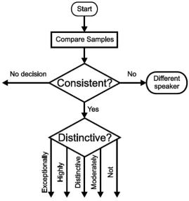
[image:42.595.184.454.301.588.2]

casework.

Figure 2.1: Flow chart of the UK Position Statement framework for FVC evidence

(from Rose and Morrison 2009: 143)

UKPS consists of a two-stage evaluation (Figure 2.1). The first stage requires an

assessment of the similarity between the suspect and offender samples, termed the

consistency judgement. It allows experts to reach one of three mutually exclusive

conclusions: consistent, not consistent or no decision. According to French and

(43)

between the samples can be explained by “established models of acoustic, phonetic

or linguistic variation” (p. 141). If the two samples are judged to be consistent, the

expert moves to the second stage, termed the distinctiveness judgement. This is an

assessment of the typicality of the shared features across the samples within the wider

population since, as Nolan (2001) states, strength of evidence is dependent on “whether

the values found matching . . . are vanishingly rare, or sporadic, or near universal in the

general (relevant) population” (p. 16). Distinctiveness is classified using the following

five-point scale:

5. Exceptionally distinctive - the possibility of this combination of features being

shared by other speakers is considered to be remote

4. Highly distinctive

3. Moderately distinctive

2. Distinctive

1. Not distinctive

from French and Harrison (2007: 141)

Distinctiveness is, for the majority of variables, assessed qualitatively. That is, while the

analysis of the samples may involve quantification of acoustic variables, their typicality

is assessed based on the expert’s knowledge and professional experience, or with

reference to published studies of sociolinguistic variation. When applying the UKPS,

the “general (relevant) population” (Nolan 2001: 16) used to assess distinctiveness is

defined according to the regional and social groups to which the expert believes the

offender belongs.

UKPS has been signed by 25 forensic practitioners and interested academics. According

to Gold and French (2011), UKPS is currently employed by 11 (32%) of the 34

practitioners surveyed and has largely replaced classical probability scales in the UK.

With the exception of one expert, the combined auditory and acoustic approach is the