Analysis of Double Ring Resonators using Method of Equating Fields

Rochester Institute of Technology

RIT Scholar Works

Theses Thesis/Dissertation Collections

7-20-2015

Analysis of Double Ring Resonators using Method

of Equating Fields

Shahana Althaf

Follow this and additional works at:http://scholarworks.rit.edu/theses

Recommended Citation

Analysis of Double Ring

Resonators using Method of

Equating Fields

Shahana Althaf

Thesis Prepared for the Degree of

Master of Science in Telecommunications Engineering Technology

Thesis Advisor

Drew N. Maywar, Ph.D.

Electrical, Computer and Telecommunications Engineering Technology College of Applied Science and Technology

Rochester Institute of Technology Rochester, NY

Abstract

Analysis Of Double Ring

Resonators Using Method of

Equating Fields

Shahana Althaf

Optical ring resonators have the potential to be integral parts of large scale

photonic circuits. My thesis theoretically analyzes parallel coupled double

ring resonators (DRRs) in detail. The analysis is performed using the method

of equating fields (MEF) which provides an in depth understanding about

the transmitted and reflected light paths in the structure. Equations for the

transmitted and reflected fields are derived; these equations allow for unequal

ring lengths and coupling coefficients. Sanity checks including comparison

with previously studied structures are performed in the final chapter in order

Acknowlegements

Let me begin by thanking almighty Allah for giving me the opportunity

to return to college and continue my education after being a mother.

I would like to dedicate my sincere gratitude to my thesis advisor Prof.

Drew Maywar for his continuous support and guidance throughout my

grad-uate study at RIT. I will always be grateful to him for helping me identify

my research interests and inspiring me to take up the challenge of doing a

thesis. His dedication and sincerity has always been an inspiration to me. I

consider my research experience with him as a valuable asset as I embark on

my doctoral studies in the next academic year.

Special thanks to Prof. Indelicato and Prof. Carlos Diaz Acosta for taking

time from their busy schedule to be on my thesis committee. Thanks again

to Prof. Indelicato for giving me the opportunity to work as his teaching

assistant.

Next I would like to thank my husband without whose support none of

this would have been possible. Thanks to him for believing in me. Thanks

to my son for letting me be with my books even when he needed me.

Thanks to my family, especially my father who brought up his daughters

with their education as the top priority. Thanks to my mother, for her

prayers.

Finally a special thanks to my sis and bro-in law and to my little niece who

Dedication

To my ikka.. thank you.. for all that you are and for all that you do

Contents

Table of Contents . . . 2

1 Ring Resonator, Single Bus Waveguide 9 1.1 Introduction . . . 9

1.2 Background . . . 10

1.3 Single Ring Resonator . . . 12

1.4 Output Electric Field . . . 13

1.5 Transmittivity . . . 15

1.5.1 Transmittivity plot for single ring resonator as a func-tion of wavelength . . . 16

1.6 Phase Transfer Function . . . 19

1.6.1 Phase Transfer Function plot for single ring resonator as a function of wavelength . . . 22

2 Uncoupled Double Ring Resonator,Single Bus Waveguide 26 2.1 Output Electric Field . . . 28

2.1.2 Ring Resonator transmission Coefficient . . . 29

2.1.3 Total transmission Coefficient . . . 30

2.2 Transmittivity . . . 30

2.2.1 Transmittivity plot for uncoupled double ring resonator as a function of wavelength . . . 31

3 Serially Coupled Double Ring Resonator, Single Bus Waveg-uide 35 3.1 Output Electric Field . . . 37

3.2 Transmittivity . . . 43

3.2.1 Transmittivity plot for single ring resonator as a func-tion of wavelength . . . 45

4 Double Ring Resonator-Transmitted field 49 4.1 Output Electric Field . . . 51

4.1.1 Only ˜E fields . . . 52

4.1.2 Only ˜F fields . . . 53

4.1.3 Mixed ˜E and ˜F fields . . . 54

4.2 Equation for ˜E2 00 based on ˜E1 only . . . 54

4.3 Equation for ˜E4 0 based on ˜E1 only (path 2) . . . 58

4.3.1 Solving for ˜F2 0 (the ring) . . . 58

4.3.2 Solving for ˜E3 . . . 61

4.4.2 Solving for ˜F2 in terms of ˜E1 . . . 65

4.4.3 Solving for ˜F4 0 in terms of ˜E1 and ˜E3 00 . . . 68

4.4.4 Solving for ˜E2 0 in terms of ˜E1 and ˜E3 00 . . . 68

4.4.5 Solving for E˜3 00 in terms of ˜E2 and ˜E2 0 . . . 69

4.4.6 Solving for ˜E2 in terms of ˜E1 . . . 70

4.4.7 Solving for ˜E2 0 in terms of ˜E1 . . . 72

4.5 Combining equations for ˜E4 0 and ˜E2 0 to obtain output electric field ˜E2 00 in terms of ˜E1 only . . . 75

4.6 Transmittivity plot based on numerical expression . . . 77

5 Double Ring Resonator-Reflected Field 79 5.1 F˜1 based on ˜F3 0 and ˜F1 0 . . . 79

5.1.1 Equation for ˜F3 0 based on ˜F1 0 , ˜E1 and ˜E4 . . . 81

5.2 Solving for ˜F1 in terms ofF10, ˜E1 and ˜E4 . . . 87

5.3 Solving for F₁0 in terms of ˜E1 and ˜E4 . . . 89

5.4 F˜1 in terms of ˜E1 and ˜E4 . . . 91

5.4.1 Solving for ˜F1 in terms of ˜E1 only . . . 94

5.5 Reflectivity plot based on numerical expression . . . 97

6 Sanity Checks 99 6.1 Sanity check for transmission equation . . . 100

6.1.1 2 = 3 = 0 . . . 100

6.1.2 1 =3 = 0 . . . 102

6.2.1 1, 2 or 3 = 0 . . . 104

6.2.2 Matching known results . . . 104

6.3 Conservation of power |r˜|2_+|˜t|2 _{= 1 . . . 106}

List of Figures

1.1 Ring resonator with single ring and single bus waveguide . . . 12

1.2 Transmittivity plot of a ring resonator as a function of

wavenum-ber under zero loss condition. . . 17

1.3 Transmittivity plot of a ring resonator where tansmittivity is

calculated as ˜tט_t? _{. . . . 19}

1.4 Phase plot of a single ring resonator as a function of

wavenum-berunder zero loss condition . . . 23

1.5 Phase plot of a single ring resonator where phase is calculated

as angle(˜t) . . . 24

2.1 Uncoupled Double Ring Resonator with single bus waveguide . 27

2.2 Transmittivity plot of an uncoupled double ring resonator

based on analytic expression . . . 33

2.3 Transmittivity plot of an uncoupled double ring resonator

where transmittivity is calculated as ˜tט_t? _{. . . . 34}

3.2 Transmittivity plot of a serially coupled DRR under zero loss

condition. . . 46

3.3 Transmittivity plot of a ring resonator where tansmittivity is

calculated as ˜tטt? . . . 48

4.1 Schematic of the DRR, showing electric fields in the counter

clockwise direction . . . 50

4.2 Schematic of the DRR, showing electric fields in the clockwise

direction . . . 50

4.3 Schematic of DRR showing light path 1 in the forward direction 56

4.4 Schematic of DRR showing light path 2 in the forward direction 57

4.5 DRR, figure showing light path3 in the forward direction . . . 57

4.6 Transmittivity plot of a DRR where transmittivity is

calcu-lated as ˜tט_t? _{. . . . 78}

5.1 Schematic of DRR showing light path 1 and 2 in the backward

direction . . . 81

5.2 Reflectivity plot of a DRR where reflectivity R is calculated

as ˜r×r˜? _{. . . . 98}

6.1 fig 3 , Chremmos and Uzunoglu (2005). . . 105

6.2 Reflectivity plot at 1 =2 = 0.1 and 3 = 0.05,0.016,0.0028. . 106

Chapter 1

Ring Resonator, Single Bus

Waveguide

1.1

Introduction

The study and characterization of optical ring resonators have developed as a

major area of research due to their potential to become integral components

of large scale photonic circuits. Ring resonator devices are comprised of bus

waveguides and rings made out of bent optical waveguides. The path where

the bus and the ring come close to one another can be regarded as a coupler,

where the interaction path (coupler length) of the optical field in the ring

and bus waveguide can be short. The principle of operation of coupling can

be based on evanescent-field coupling, although multimode interference also

Different configurations of multiple ring resonators are found to exhibit

filtering characteristics which are desirable in WDM applications. They find

applications as wavelength selective filters such as add-drop filters or band

rejection filters in photonic circuits. The ease of fabrication into intergrated

circuits has been recognized as the major advantage of optical filters based

on ring resonators.

1.2

Background

A theoretical analysis of a basic ring resonator configuration consisting of one

waveguide and a single ring was presented by A.Yariv in 2000. The

funda-mental working equations describing the general behavior of a basic resonator

filter were derived and the applicability as filters were discussed. The analysis

was performed using matrix relations considering single polarization under

lossless conditions [1].

In 2004, a new type of reflector consisting of a circular array of micro

ring resonators coupled to a waveguide was proposed and analyzed [2]. The

transmittance and reflectance of the structure was computed using transfer

matrix analysis. It was proved that the structure acted as an all pass filter

for an even number of rings. Although different geometries of multiple ring

Double ring-resonators (DRRs) composed of just two micro-rings and

a straight waveguide which are coupled to each other was studied for the

first time in 2005 and was proved to be a good reflector [4]. Scattering

matrix formalism was used to prove that a range of reflectivity profiles can

be obtained by tuning the coupling coefficients. Another study of DRRs with

rings having slightly different radii was reported a year later [3] [5].

DRRs have many advantages over the previously reported structures. As

it consists of only two rings, which simplifies the fabrication process, this

resonator can replace distributed Bragg reflectors used in realizing tunable

laser diodes [9] [6] [7] [8]. In order to exploit all the functionalities of this

structure, a deep understanding of its characteristics is necessary.

The method of equating fields (MEF) provides a deeper understanding

of the light path and the propagation of the electric fields taking place in

the structure. The method yields several equations consisting of components

representing the path followed by light as it travels along the structure. The

results of the analysis includes equations for transmission and reflection

coef-ficients ˜t, ˜r. The circumference of the rings L1 is not assumed to be equal to

L2 and coupling coefficients1 is not equal to2 in the solution. An analysis

is performed on simpler structures in the early chapters in order to compare

1.3

Single Ring Resonator

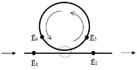
In the basic configuration, a ring resonator consists of a single bus waveguide

coupled to a single ring made of a bent waveguide as shown in Figure 1.1.

The arrow indicates the direction of propagation of light and the thin line

indicates the coupling region.

Figure 1.1: Ring resonator with single ring and single bus waveguide

When light through the bus waveguide enters the region where the ring is

close to the bus waveguide it is coupled to the ring resonator through

evanes-cent coupling. The light entering the ring travels along the circumference of

the ring and enters the coupling region again. Exchange of power takes place

at the coupling region due to the interaction between the optical field in the

ring and the bus waveguide. Here ˜E1 is the input electric field to the coupler

1.4

Output Electric Field

The output electric field ˜E2 is given as

˜

E2 = ˜E1

√

1−+ ˜E4 i

√

, (1.1)

˜

E4 = ˜E3 eiβL, (1.2)

˜

E3 =i

√

E˜1+

√

1− E˜4, (1.3)

whereL is the circumference of the entire ring.

Combining Equations (1.2) and (1.3) yields

˜

E4 =i

√

eiβL E˜1+

√

1− eiβL E˜4,

(1−√1− eiβL) ˜E4 =i

√

eiβL E˜1,

˜

E4 =

i√ eiβL

(1−√1− eiβL₎

˜

The equation for ˜E2 becomes

˜

E2 = ˜E1[

√

1−+ i

√

i√ eiβL

1−√1− eiβL],

˜

E2 = ˜E1[

√

1−−(1−) eiβL− eiβL

1−√1− eiβL ],

˜

E2 = ˜E1[

√

1−−eiβL_{+ e}iβL_{− e}iβL

1−√1− eiβL ],

˜

E2 = ˜E1[

√

1−−eiβL

1−√1− eiβL],

˜

E2 = ˜E1[

√

1− e−iβL₋₁

1−√1− eiβL ] e iβL_,

˜

E2 = ˜E1[

1−√1− e−iβL

1−√1− eiβL ] e

iβL _eiπ_{. (1.5)}

We know

˜

Therefore the transmission coefficient ˜t is

˜

t= [1−

√

1− e−iβL

1−√1− eiβL ] e iβL

eiπ. (1.6)

1.5

Transmittivity

Transmittivity of a medium is defined as the ratio of transmitted power to

the incident power:

T =|E˜2

˜

E1

|2 _=|˜t|2_{. (1.7)}

The above equation is rewritten as,

T = (

√

1−−eiβL₎₍√_1−−e−iβL₎

(1−√1− eiβL₎₍₁₋√_{1− e}−iβL₎,

T = (1−) + (1−

√

1− eiβL₎₋₍√_{1− e}−iβL₎

1 + (1−)−(√1− eiβL₎₋₍√_{1− e}−iβL₎,

T = 2−−2

√

1− cos(βL)

2−−2√1− cos(βL) = 1. (1.8)

Here, transmittivity is equal to one which means that the total power

entering and leaving the ring resonator are equal. The unity value of

trans-mittivity shows that under loss-less conditions, there are no spectral features

resonator passes through it.

1.5.1

Transmittivity plot for single ring resonator as a

function of wavelength

A sanity check on the derived equations is performed by comparing the graphs

obtained by plotting transmittivityT based on both analytical and numerical

techniques.

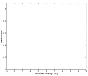
Transmittivity plot based on analytic expression TA

TA=

(√1−−eiβL₎₍√_1−−e−iβL₎

(1−√1− eiβL₎₍₁₋√_{1− e}−iβL₎.

The figure shows the transmittivity of a single ring resonator plotted as a

function of the normalised product βL where β is the wavenumber and L is

Figure 1.2: Transmittivity plot of a ring resonator as a function of wavenum-ber under zero loss condition.

The equation derived for transmittivity is used for plotting the graph.

We can see that under lossless conditions, the transmittivity is equal to one

which indicates that the total power entering and leaving the coupling region

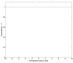
Transmittivity plot based on numerical expression TN

We know transmittivity is the product of the transmission coefficient ˜t and

its conjugate ˜t?_.

TN = ˜t × ˜t?.

where,

˜

t= [1−

√

1− e−iβL

1−√1− eiβL ] e

iβL _eiπ_.

The figure shows the response obtained when ˜t × ˜t? is plotted againstβL.

We can see that the plots from both the analytic and numerical expressions

Figure 1.3: Transmittivity plot of a ring resonator where tansmittivity is calculated as ˜tטt?

1.6

Phase Transfer Function

The phase transfer function of the ring resonator is composed of three parts:

φT =arg

˜

E2

˜

E1

!

,

where x is the phase of the bracketed termB in equation (1.5), where

B = 1−

√

1− e−iβL

1−√1− eiβL .

The phase xcan be determined by multiplication of B and a unity ratio

whose denominator turns the resulting denominator into a real quantity.

B = (1−

√

1− e−iβL₎

(1−√1− eiβL₎ ∗

(1−√1− e−iβL₎

(1−√1− e−iβL₎

B = (1−

√

1− e−iβL₎2

(2−−2√1−cos(βL)),

B = (1−

√

1− cos(βL) +i √1− sin(βL))2

D ,

where,

D= 2−−2√1−cos(βL).

B can be written as (a+i b)2_{, where}

a= 1−

√

1− cos(βL)

√

D ,

We desire to know the phase x of B, where

B = (a+ib)2,

but x is related to the phase of

√

B =a+ib.

In general, the Cartesian and phasor representations of a complex quantity

are given as:

a+ib=m eiθ,

(a+ib)2 = (m eiθ)2 =m2 ei2θ =G eix,

where,

x= 2θ.

Thus, the square of a complex quantity is equivalent to a new complex

B can be found as

tan(θ) = b

a =

√

1− sin(βL) 1−√1− cos(βL),

θ = tan−1(

√

1− sin(βL) 1−√1− cos(βL)),

x= 2θ = 2 tan−1

√

1− sin(βL) 1−√1− cos(βL)

. (1.9)

The phase transfer function is

φT =x+π+βL.

Substituting x from equation (1.8), yields

φT = 2 tan−1

√

1− sin(βL) 1−√1− cos(βL)

+π+βL. (1.10)

1.6.1

Phase Transfer Function plot for single ring

res-onator as a function of wavelength

A sanity check on the derived equation is performed by comparing the graphs

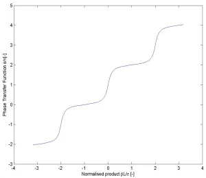
ex-Phase plot based on analytic expression φTA

Figure 1.4: Phase plot of a single ring resonator as a function of wavenum-berunder zero loss condition

The figure shows the phase transfer function of a single ring resonator

based on the analytic expression (1.9), plotted as a function of the normalised

product βL where β is the wavenumber and L is the circumference of the

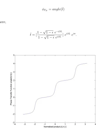
Phase Transfer function based on numerical expression φTN

We know,

φTN =angle(˜t)

where,

˜

t= [1−

√

1− e−iβL

1−√1− eiβL ] e

The figure shows the response obtained when angle(˜t) is plotted against

βL. We can see that the plots obtained using both analytic and numerical

Chapter 2

Uncoupled Double Ring

Resonator,Single Bus

Waveguide

Double Ring Resonators are coupled ring resonator devices consisting of two

ring waveguides coupled to one or more bus waveguides. The Double Ring

Resonator shown in Figure 2.1 is comprised of two ring waveguides of

cir-cumference L1 andL2 coupled to a same single bus waveguide. The rings are

spaced apart and are not coupled to each other. The space where the rings

are close to the bus waveguide creates two coupling regions separated by a

Figure 2.1: Uncoupled Double Ring Resonator with single bus waveguide

Light entering the bus waveguide is coupled to the first ring through

evanescent coupling and travels along the circumferenceL1 of the ring before

entering the same coupling region again. Transfer of power takes place at

the coupling region. The light leaving the region travels a distance of Ls

along the bus waveguide to enter the region where the second ring is coupled

to the bus waveguide. Through evanescent coupling light enters the second

ring, travels along its circumference L2 and re enters the coupling region.

Here ˜E1 is the input electric field to the coupler and ˜E4 is the input from the

first ring to the coupler. ˜E3 is the output electric field from the coupler along

the first ring and ˜E2 is the output from the first coupling region along the

bus waveguide. E˜0

1 is the input electric field to the second coupling region

and ˜E0

4 is the input from the second ring to the coupler. E˜30 is the output

electric field from the coupler along the second ring and ˜E0

2 is the output

2.1

Output Electric Field

The electric fields ˜E₁0 , ˜E2 and ˜E20 are given as,

˜

E2 = ˜tL1 E˜1

˜

E₁0 = ˜tLs E˜2

˜

E₂0 = ˜tL2 E˜

0

1

where ˜tL1, ˜tLs and ˜tL2 are transmission coefficients of the first coupling region,

the space between the two coupling regions and the second coupling region

respectively. Therefore, ˜E0

2 is

˜

E₂0 =t E˜1. (2.1)

where

˜

t= ˜tL1.t˜Ls. ˜tL2. (2.2)

2.1.1

Bus Wave guide transmission Coefficient

The equation for electric field ˜E₁0 is

˜

Therefore

˜

tLs =e

iβLs_{. (2.3)}

2.1.2

Ring Resonator transmission Coefficient

We have

˜

E2 = ˜E1

1−p

(1−1) e−iβL1

1−p(1−1) eiβL1

!

eiβL1 _eiπ_.

Therefore

˜

tL1 =

1−p(1−1) e−iβL1

1−p(1−1) eiβL1

!

eiβL1 _eiπ_{. (2.4)}

Likewise,

˜

E₂0 = ˜E₁0 1−

p

(1−2) e−iβL2

1−p(1−2)eiβL2

!

eiβL2 _eiπ_{. (2.5)}

Therefore

˜

tL2 =

1−p

(1−2)e−iβL2

1−p

(1−2)eiβL2

!

2.1.3

Total transmission Coefficient

˜

t= ˜tL1.t˜Ls. ˜tL2.

Substituting the values of ˜tL1,˜tLs and ˜tL2 in the above equation yields

˜

t = 1−

p

(1−1)e−iβL1

1−p(1−1) eiβL1

!

eiβL1_eiπ_eiβLs 1−

p

(1−2) e−iβL2

1−p(1−2) eiβL2

!

eiβL2 _eiπ_,

˜

t= 1−

p

(1−1) e−iβL1

1−p

(1−1) eiβL1

!

eiβ(L1+Ls+L2) _ei2π 1−

p

(1−2) e−iβL2

1−p

(1−2) eiβL2

!

,

˜

t = 1−

p

(1−1)e−iβL1

1−p(1−1)eiβL1

!

eiβ(L1+Ls+L2) 1−

p

(1−2) e−iβL2

1−p(1−2) eiβL2

!

.

(2.7)

2.2

Transmittivity

Transmittivity is the ratio of transmitted power to incident power:

T =|E˜

0

2

˜

E1

The total transmittivity is related to the constituent transmittivities as

fol-lows

T =T2.Ts.T1 (2.9)

where

T1 =

(√1−1−eiβL1) (

√

1−1−e−iβL1)

(1−√1−1 eiβL1) (1−

√

1−1 eiβL1)

= 1,

T2 =

(√1−2−eiβL2) (

√

1−2−e−iβL2)

(1−√1−2 eiβL2) (1−

√

1−2 eiβL2)

= 1,

Ts= (eiβLs) (e−iβLs) = 1.

Therefore the total transmittivity is equal to one under loss less conditions.

2.2.1

Transmittivity plot for uncoupled double ring

resonator as a function of wavelength

A sanity check on the derived equations is performed by comparing the graphs

obtained by plotting transmittivityT based on both analytical and numerical

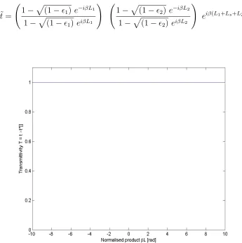
Transmittivity plot based on analytic expression TA

T =TA2.TAs.TA1 (2.10)

where

TA1 =

(√1−1−eiβL1) (

√

1−1−e−iβL1)

(1−√1−1 eiβL1) (1−

√

1−1 eiβL1)

,

TA2 =

(√1−2−eiβL2) (

√

1−2−e−iβL2)

(1−√1−2 eiβL2) (1−

√

1−2 eiβL2)

,

TAs = (e

iβLs_{) (e}−iβLs_).

The figure shows the transmittivity plot of an uncoupled double ring

resonator plotted as a function of the normalised product βLwhere β is the

Figure 2.2: Transmittivity plot of an uncoupled double ring resonator based on analytic expression

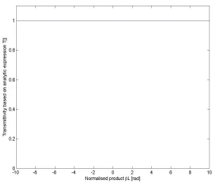
Transmittivity plot based on numerical expression TN

We know transmittivity is the product of the transmission coefficient ˜t and

its conjugate ˜t?_.

where,

˜

t= 1−

p

(1−1) e−iβL1

1−p(1−1) eiβL1

!

1−p

(1−2)e−iβL2

1−p(1−2)eiβL2

!

eiβ(L1+Ls+L2)_.

Figure 2.3: Transmittivity plot of an uncoupled double ring resonator where transmittivity is calculated as ˜t×_t˜?

The figure shows the response obtained when ˜t × ˜_t? _{is plotted againstβL.}

We can see that the plots from both the analytic and numerical expressions

Chapter 3

Serially Coupled Double Ring

Resonator, Single Bus

Waveguide

The structure consists of two ring optical waveguides coupled serially to a

single bus waveguide. The first ring of circumference L1is directly coupled

to the waveguide while the second ring of circumference L2 is coupled to

the first ring through evanascent coupling. This creates two coupling regions

-one between the first ring and the bus waveguide and one between the two

rings. Light entering the waveguide is coupled to the first ring at the region

where the ring is close to the waveguide. Light coupled to the ring through

evanascence, travels along its circumference and enters the second coupling

Figure 3.1: Double Ring Resonator coupled serially to a single bus waveguide

evanascent coupling light enters the second ring, travels along its

circumfer-ence L2 and re-enters the second coupling region to be coupled back to the

first ring.It travels along the circumference L1 of the first ring and re enters

the first coupling region and exits along the bus waveguide.

Here ˜E1 is the input electric field to the coupler and ˜E4 is the input from

the first ring to the coupler. ˜E3 is the output electric field from the coupler

along the first ring and ˜E2 is the output from the first coupling region along

3.1

Output Electric Field

The equations for electric fields at the two coupling regions are given as

˜

E3 =i

√

1 E˜1+

√

1−1 E˜4, (3.1)

˜

E2 = ˜E1

√

1−1 + ˜E4 i

√

1, (3.2)

˜

E1

0

=√1−2 E˜2

0

+i√2 E˜3

0

, (3.3)

˜

E2

0

= ˜E1

0

eiβL2_{, (3.4)}

˜

E4

0

=i√2 E˜2

0

+√1−2 E˜3

0

. (3.5)

˜

E3

0

= ˜E3 eiβL1/2. (3.6)

˜

E4 = ˜E4

0

Combining Equations (3.5) and (3.7) yields

˜

E4 = (i

√

2 E˜2

0

+√1−2 E˜3

0

) eiβL1/2_{. (3.8)}

Combining Equations (3.6) and (3.8) yields

˜

E4 =i

√

2 E˜2

0

eiβL1/2₊√₁₋

2 E˜3 eiβL1. (3.9)

Replacing ˜E3 in the above equation with Equation (3.1) gives

˜

E4 =i

√

2 E˜2

0

eiβL1/2 _+i√

1

√

1−2E˜1 eiβL1

+√1−1

√

1−2 E˜4 eiβL1,

˜

E4(1−

p

(1−1) (1−2) eiβL1) =i

√

2 E˜2

0

eiβL1/2_+i√

1

√

1−2 E˜1 eiβL1.

Combining Equations (3.3) and (3.4) yields

˜

E2

0

= (√1−2 E˜2

0

+i√2 E˜3

0 eiβL2_,

˜

E2

0

= i

√

2 E˜3

0 eiβL2

1−√1−2 eiβL2

.

Replacing ˜E3

0

in the above equation with Equation (3.6) yields

˜

E2

0

= i

√

2 E˜3 eiβL1/2eiβL2

1−√1−2 eiβL2

. (3.11)

Combining Equations (3.1) and (3.11) yields

˜

E2

0

= −

√

2 1 eiβL1/2 eiβL2 E˜1+ 1

p

2(1−1) eiβL1/2 eiβL2 E˜4

1−√1−2 eiβL2

Combining Equations (3.12) and (3.10) yields

˜

E4 (1−

p

(1−1) (1−2)eiβL1) = i

p

1 (1−2) ˜E1 eiβL1+

i√2 eiβL1/2

ip2(1−1) eiβL2 eiβL1/2 E˜4−

√

1 2 eiβL2 e1βL1/2 E˜1

1−√1−2 eiβL2

!

,

˜

E4 =

ip(1−2)1 eiβL1 E˜1(1−

√

1−2eiβL2)

−2

√

1−1 eiβL1 eiβL2 E˜4−i

√

1 2 eiβL1 eiβL2 E˜1

(1−√1−2 eiβL2) (1−

p

(1−1)(1−2) eiβL1)

,

˜

E4 1 +

2

√

1−1 eiβL1 eiβL2

(1−√1−2 eiβL2) (1−

p

(1−1)(1−2) eiβL1)

!

=

˜

E1

ip1(1−2) eiβL1 −i(1−2)

√

1 eiβL1 eiβL2 −i

√

1 2 eiβL1 eiβL2

(1−√1−2 eiβL2) (1−

p

(1−1)(1−2) eiβL1)

!

,

˜

E4

(1−√1−2 eiβL2) (1−

p

(1−1)(1−2)eiβL1) +2

√

1−1 eiβL1 eiβL2

(1−√1−2 eiβL2) (1−

p

(1−1)(1−2) eiβL1)

!

=

˜

E1

ip1(1−2) eiβL1 −i(1−2)

√

1 eiβL1 eiβL2 −i

√

1 2 eiβL1 eiβL2

(1−√1−2 eiβL2) (1−

p

(1−1)(1−2) eiβL1)

!

,

˜

E4 = ˜E1

ip1(1−2) eiβL1−i(1−2)

√

1 eiβL1 eiβL2 −i

√

1 2 eiβL1 eiβL2

(1−√1−2 eiβL2) (1−

p

(1−1)(1−2) eiβL1) +2

√

1−1 eiβL1 eiβL2

!

˜

E4 = ˜E1

ip1(1−2) eiβL1 −i

√

1 eiβL1 eiβL2

1−p(1−1) (1−2)eiβL1 −

√

1−2 eiβL2 +

√

1−1 eiβL2 eiβL1

!

.

(3.13)

We know

˜

E2 = ˜E1

√

1−1+ ˜E4 i

√

1. (3.14)

Combining Equations (3.13) with the Equation for ˜E2 yields

˜

E2 =i

√

1E˜1

ip1(1−2) eiβL1 −i

√

1 eiβL1 eiβL2

1−p

(1−1) (1−2)eiβL1 −

√

1−2 eiβL2 +

√

1−1 eiβL2 eiβL1

!

+

˜

E1

√

1−1,

˜

E2 = ˜E1

         √

1−1

1−p

(1−1) (1−2)eiβL1 −

√

1−2 eiβL2 +

√

1−1 eiβL1 eiβL2

+

i√ ip1(1−2)eiβL1 −i

√

1 eiβL1 eiβL2

1−p

(1−1) (1−2) eiβL1 −

√

1−2 eiβL2 +

√

1−1 eiβL2 eiβL1

         , ˜

E2 = ˜E1

√

1−1−

√

1−2 eiβL1 −

p

(1−1) (1−2)eiβL2 +eiβL2 eiβL1

1−p(1−1) (1−2)eiβL1 −

√

1−2 eiβL2 +

√

1−1 eiβL2 eiβL1

!

˜

E2 = ˜E1

√

1−1 e−iβL2 e−iβL1 −

√

1−2 e−iβL2 −

p

(1−1) (1−2) e−iβL1 + 1

1−p

(1−1) (1−2)eiβL1 −

√

1−2 eiβL2 +

√

1−1 eiβL2 eiβL1

!

eiβ(L1+L2)_,

˜

E2 = ˜E1

√

1−2 e−iβL2 −

√

1−1 e−iβL2e−iβL1 +

p

(1−1)(1−2)e−iβL1 −1

1−p(1−1)(1−2)eiβL1 −

√

1−2 eiβL2 +

√

1−1 eiβL2 eiβL1

!

eiβ(L1+L2)_eiπ_.

(3.15)

We know

˜

E2 = ˜t E˜1

Therefore the transmission coefficient ˜t is

˜

t =

√

1−2 e−iβL2 −

√

1−1 e−iβL2e−iβL1 +

p

(1−1)(1−2)e−iβL1 −1

1−p(1−1)(1−2)eiβL1 −

√

1−2 eiβL2 +

√

1−1 eiβL2 eiβL1

!

eiβ(L1+L2) _eiπ_.

(3.16)

When 2 = 0, the output electric field becomes,

˜

E2 = ˜E1

√

1−1−eiβL1 −

√

1−1 eiβL2 +eiβ(L1+L2)

1−√1−1 eiβL1−eiβL2 +

√

1−1 eiβ(L1+L2)

,

˜

E2 = ˜E1

√

1−1(1−eiβL2)−eiβL1(1−eiβL2)

(1−eiβL2)−√1−

1 eiβL1(1−eibetaL2)

,

which is same as Equation(1.5) which gives the output electric field of a single

ring resonator coupled to a single bus waveguide.

When 1 = 0, the output electric field becomes,

˜

E2 = ˜E1

1−√1−2 eiβL1 −

√

1−2 eiβL2 +eiβ(L1+L2)

1−√1−1 eiβL1 −

√

1−2 eiβL2 +eiβ(L1+L2)

That is,

˜

E2 = ˜E1.

3.2

Transmittivity

Transmittivity is the ratio of transmitted power to the incident power:

T =|E˜2

˜

E1

The above equation is rewritten as,

T =

√

1−2 e−iβL2 −

√

1−1 e−iβ(L1+L2)+

p

(1−1)(1−2)e−iβL1 −1

1−p(1−1)(1−2)eiβL1 −

√

1−2 eiβL2 +

√

1−1 eiβ(L1+L2)

!

×

√

1−2 eiβL2 −

√

1−1 eiβ(L1+L2)+

p

(1−1)(1−2)eiβL1 −1

1−p(1−1)(1−2)e−iβL1−

√

1−2 e−iβL2 +

√

1−1 e−iβ(L1+L2)

!

,

T =

(1−2)−

p

(1−1) (1−2)(eiβL1 +e−iβL1) + (1−2)

√

1−1(eiβ(L1−L2)+e−iβ(L1−L2)

−√1−2(eiβL2 +e−iβL2) + (1−1)

−(1−1)

√

1−2(eiβL2 +e−iβL2) + (1−1)(1−2)

+√1−1(eiβ(L1+L2)+e−iβ(L1+L2)

−p

(1−1)(1−2)(eiβL1 +e−iβL1) + 1

1−p(1−1) (1−2)(eiβL1 +e−iβL1)−

√

1−2(eiβL2 +e−iβL2)

+p(1−1)(eiβ(L1+L2)+e−iβ(L1+L2))−(1−1)

√

1−2(eiβL2 +e−iβL2)

+(1−1)(1−2) + (

√

1−1)(1−2)(eiβ(L1−L2)+e−iβ(L1−L2)

+(1−2) +

p

(1−1)(1−2)(eiβL1+e−iβL1)

+ (1−1)

,

T =

3−1−2+ (1−1)(1−2) + (1−2)

√

1−1 cos(β(L1−L2))−

√

1−2 cos(βL2)

−(1−1)

√

1−2 cos(βL2) +

√

1−1cos(β(L1+L2))

3−1−2+ (1−1)(1−2) + (1−2)

√

1−1 cos(β(L1−L2))−

√

1−2 cos(βL2)

−(1−1)

√

1−2 cos(βL2) +

√

1−1cos(β(L1+L2))

= 1.

which shows that under loss less conditions, total power entering the coupling

3.2.1

Transmittivity plot for single ring resonator as a

function of wavelength

A sanity check on the derived equations is performed by comparing the graphs

obtained by plotting transmittivityT based on both analytical and numerical

techniques.

Transmittivity plot based on analytic expression TA

T =

√

1−2 e−iβL2 −

√

1−1 e−iβ(L1+L2)+

p

(1−1)(1−2)e−iβL1 −1

1−p

(1−1)(1−2)eiβL1 −

√

1−2 eiβL2 +

√

1−1 eiβ(L1+L2)

!

×

√

1−2 eiβL2 −

√

1−1 eiβ(L1+L2)+

p

(1−1)(1−2)eiβL1 −1

1−p(1−1)(1−2)e−iβL1 −

√

1−2 e−iβL2 +

√

1−1 e−iβ(L1+L2)

!

.

The figure shows the transmittivity of a single ring resonator plotted as

a function of the normalised product βL where β is the wavenumber and L

Figure 3.2: Transmittivity plot of a serially coupled DRR under zero loss condition.

The equation derived for transmittivity is used for plotting the graph.

We can see that under lossless conditions, the transmittivity is equal to one

which indicates that the total power entering and leaving the coupling region

Transmittivity plot based on numerical expression TN

We know transmittivity is the product of the transmission coefficient ˜t and

its conjugate ˜t?_.

TN = ˜t × ˜t?.

where,

˜

t=

√

1−1−

√

1−2 eiβL1 −

p

(1−1) (1−2)eiβL2 +eiβL2 eiβL1

1−p(1−1) (1−2)eiβL1 −

√

1−2 eiβL2 +

√

1−1 eiβL2 eiβL1

!

.

The figure shows the response obtained when ˜t × ˜_t? _{is plotted againstβL.}

We can see that the plots from both the analytic and numerical expressions

Chapter 4

Double Ring

Resonator-Transmitted field

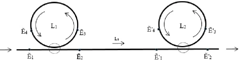
The double ring resonator (DRR) consists of two mutually coupled rings

coupled to a single bus waveguide. There are three coupling regions in the

DRR, one between the rings and the other two between each ring and the

bus waveguide. L1 and L2 are the circumference of the rings and Ls is the

space between the coupling regions 1 and 2.

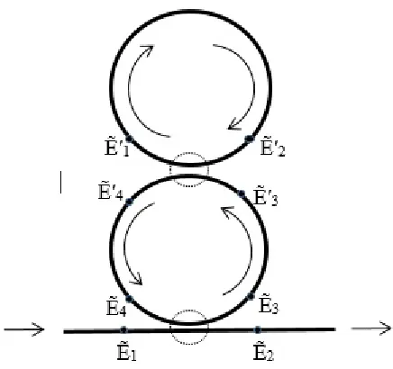
Light propagates in both forward and backward direction as the rings are

mutually coupled to each other. There are a total of 24 field points at both

ends of the three coupling regions including the input field ˜E1 , as shown in

Figure (1.1) and (1.2). ˜E represents an electric field in the counter clockwise

direction and ˜F represents an electric field in the clockwise direction. ˜F2

00

= 0

electric fields are represented as linear equations, of which 10 are propagation

equations and 12 are coupling equations.

Figure 4.1: Schematic of the DRR, showing electric fields in the counter clockwise direction

4.1

Output Electric Field

4.1.1

Only

E

˜

fields

˜

E3 =i

√

1 E˜1+

√

1−1 E˜4, (4.1)

˜

E2 = ˜E1

√

1−1+ ˜E4 i

√

1, (4.2)

˜

E1

0

= ˜E3

00

eiβ 3L2/4_{, (4.3)}

˜

E3

0

= ˜E3 eiβL1/4, (4.4)

˜

E4 = ˜E4

0

eiβ 3L1/4_{, (4.5)}

˜

E3

00

= ˜E1

00

i√2+

√

1−2 E˜4

00

, (4.6)

˜

E4

00

=eiβL2/4 _E˜

2

0

, (4.7)

˜

E1

00

= ˜E2 eiβLs, (4.8)

˜

E2

00

= ˜E1

00 √

1−2+i

√

2 E˜4

00

4.1.2

Only

F

˜

fields

˜

F2

0

= ˜F4

00

eiβL2/4_{, (4.10)}

˜

F3

00

= ˜F1

0

eiβ3L2/4_{, (4.11)}

˜

F1

00

=i√2 F˜3

00

, (4.12)

˜

F4

00

=√1−2 F˜3

00

, (4.13)

˜

F4 =i

√

1 F˜2+

√

1−1 F˜3, (4.14)

˜

F4

0

=eiβ3L1/4 _F˜

4, (4.15)

˜

F3 =eiβL1/4 F˜3

0

, (4.16)

˜

F1 = ˜F3 i

√

1+

√

1−1 F˜2, (4.17)

˜

F2 =eiβLs F˜1

00

4.1.3

Mixed

E

˜

and

F

˜

fields

˜

E2

0

= ˜E1

0 √

1−3+ ˜F4

0

i√3, (4.19)

˜

E4

0

=√1−3 E˜3

0

+ ˜F2

0

i√3, (4.20)

˜

F1

0

= ˜F2

0 √

1−3+ ˜E3

0

i √3, (4.21)

˜

F3

0

= ˜F4

0 √

1−3+ ˜E1

0

i√3, (4.22)

4.2

Equation for

E

˜

00

based on

E

˜

only

The goal of this chapter is to derive an equation for the output electric field

˜

E2

00

based on the input electric field ˜E1 only. The 22 linear equations are

solved using the ’Method of Equating Fields’ in order to come up with the

final equation for ˜E2

00

. The derivation is carried out in several steps yielding

equations representing the path followed by the light as it travels along the

structure.

From Equation (4.9) we know,

˜

E2

00

= ˜E1

00 √

1−2+i

√

2 E˜4

Combining Equation(4.8) and Equation (4.9), we get

˜

E2

00

= ˜E2 eiβLs

√

1−2+i

√

2 E˜4

00 .

Combining the above Equation with Equation (4.2) for ˜E2and then equation

(4.5) for ˜E4 , we get

˜

E2

00

=eiβLs √₁₋

2 ( ˜E1

√

1−1+ ˜E4 i

√

1) +i

√

2 E˜4

00 ,

˜

E2

00

=eiβLs p₍₁₋

2) (1−1) ˜E1+eiβLs

√

1−2 i

√

1 E˜4

0

eiβ3L1/4_+i√

2 E˜4

00 .

(4.23)

And, we know from equation (4.7) that ˜E4

00

can be written in terms of ˜E2

0 , resulting in ˜ E2 00

=eiβLs p₍₁₋

2) (1−1) ˜E1+eiβLs

√

1−2 i

√

1 E˜4

0

eiβ3L1/4_+i√

2 eiβL2/4 E˜2

0 .

(4.24)

This particular equation is very important in the analysis of the DRR. The

three components of the equation for ˜E2

00

represents the three different paths

through which light propagates and exits through the DRR in the forward

direction.

The first component of the equation, eiβLs p₍₁₋

2) (1−1) ˜E1

waveguide after crossing the two coupling regions1 and2 and exits through

the waveguide. This component represents the simplest light path in a DRR

structure. Figure 4.3 below shows light path 1 in the forward direction.

Figure 4.3: Schematic of DRR showing light path 1 in the forward direction

The second component of the equation, eiβLs √₁₋

2 i

√

1 eiβ3L1/4 E˜4

0

represents the light leaving the coupling region3 between the two rings. The

light travels along 3₄ of the circumference L1 of the first ring and then enters

the two coupling regions 1 and 2, between the rings and the waveguide

before exiting through the waveguide. Figure 4.5 below shows the light path

Figure 4.4: Schematic of DRR showing light path 2 in the forward direction

The third component of the equation represents the light leaving the

coupling region 3 between the rings and travels along 1₄ of the circumference

L2 of the second ring before entering the coupling region 2 between the

second ring and the waveguide and exits through the waveguide. Figure 4.4

below shows the light path 3.

Figure 4.5: DRR, figure showing light path3 in the forward direction

The next step is to solve for ˜E4

0

and ˜E2

0

in terms of ˜E1. Doing so will

yield an equation for ˜E2

00

account. All other possible paths (such as light leaving ˜E4

0

and circulating

around ring 1 ) are accounted for by these three paths.

4.3

Equation for

E

˜

based on

E

˜

only (path

2

)

From equation (4.20) we know,

˜

E4

0

=√1−3 E˜3

0

+ ˜F2

0 i√3.

Combining the above equation with Equation (4.4), we get

˜

E4

0

=√1−3 E˜3 eiβL1/4+ ˜F2

0

i√3. (4.25)

Here the second ring acts like a ring resonator attached to the first ring. All

of its light (in the clockwise orientation) comes from the first ring.

4.3.1

Solving for

F

˜

0

(the ring)

Now we need ˜F2

0

based on ˜E3. We know from equation (4.10),

˜

F2

0

= ˜F4

00

Combining the above equation with Equations (4.13) and (4.11) yields

˜

F2

0

=√1−2 F˜3

00

eiβL2/4_,

˜

F2

0

=√1−2 eiβL2/4 F˜1

0

eiβ3L2/4_,

˜

F2

0

=√1−2 eiβL2 F˜1

0

. (4.26)

Combining Equations (4.26) and (4.21), yields

˜

F2

0

=√1−2 eiβL2 ( ˜F2

0 √

1−3+ ˜E3

0

i √3),

=p(1−2) (1−3) eiβL2 F˜2

0

+√1−2 eiβL2 E˜3

0

i √3,

˜

F2

0

(1−p(1−2) (1−3)eiβL2) =

√

1−2 eiβL2 E˜3

0

i √3,

˜

F2

0

=

" √

1−2 eiβL2 i

√

3

1−p(1−2) (1−3) eiβL2

#

˜

E3

0 .

Combining Equations (4.27) and (4.4) yields,

˜

F2

0

=

" √

1−2 eiβL2 i

√

3

1−p(1−2) (1−3) eiβL2

#

˜

E3 eiβL1/4. (4.28)

Now combining equations (4.28) and (4.24) , we get

˜

E4

0

=√1−3 E˜3 eiβL1/4+i

√

3

" √

1−2 eiβL2 i

√

3

1−p

(1−2) (1−3)eiβL2

#

˜

E3 eiβL1/4.

=

√

1−3 eiβL1/4(1−

p

(1−2) (1−3) eiβL2) ˜E3−(3

√

1−2 eiβL2 eiβL1/4) ˜E3

1−p(1−2) (1−3) eiβL2

,

=

"√

1−3 eiβL1/4−eiβ(L2+L1/4)

√

1−2

1−p

(1−2) (1−3) eiβL2

#

˜

E3,

˜

E4

0

=

" √

1−3−eiβL2

√

1−2

1−p(1−2) (1−3)eiβL2

#

eiβL1/4 _E˜

The denominator term p(1−2) (1−3) eiβL2 is simply the transmission

coefficient t2 after traversing the second ring once. Therefore,

˜

E4

0

=

√

1−3−eiβL2

√

1−2

1−t2

eiβL1/4 _E˜

3. (4.29)

Now we need ˜E3 in terms of ˜E1.

4.3.2

Solving for

E

˜

From equation (4.1), we have

˜

E3 =i

√

1 E˜1+

√

1−1 E˜4.

Combining equations (4.1) and (4.5), yields

˜

E3 =i

√

1 E˜1 +

√

1−1 E˜4

0

eiβ 3L1/4_{. (4.30)}

From equation (4.29) we have,

˜

E4

0

=

" √

1−3−eiβL2

√

1−2

1−p(1−2) (1−3)eiβL2

#

eiβL1/4 _E˜

3.

Combining equations (4.29) and (4.30) yields,

˜

E3 =i

√

1E˜1+

√

1−1eiβ 3L1/4

"√

1−3 eiβL1/4 −eiβ(L2+L1/4)

√

1−2

1−p

(1− ) (1− ) eiβL

#

˜

=i√1 E˜1+

" p

(1−1) (1−3)eiβL1 −

p

(1−1) (1−2) eiβ(L1+L2)

1−p(1−2) (1−3)eiβL2

#

˜

E3,

˜

E3 1−

" p

(1−1) (1−3)eiβL1 −

p

(1−1) (1−2) eiβ(L1+L2)

1−p

(1−2) (1−3) eiβL2

#!

=i√1E˜1,

˜

E3

1−p(1−2) (1−3) eiβL2 −

p

(1−1) (1−3)eiβL1 +

p

(1−1) (1−2)eiβ(L1+L2)

1−p(1−2) (1−3)eiβL2

!

=i√1 E˜1,

˜

E3 =

i√1(1−

p

(1−2) (1−3) eiβL2)

1−p(1−2) (1−3)eiβL2 −

p

(1−1) (1−3) eiβL1 +

p

(1−1)(1−2)eiβ(L1+L2)

!

˜

E1.

(4.31)

Combining equations (4.29) and (4.31), yields

˜

E4

0

=

"

i√1(

√

1−3 eiβL1/4−eiβ(L2+L1/4)

√

1−2)

1−p(1−2) (1−3)eiβL2 −

p

(1−1) (1−3)eiβL1 +

p

(1−1)(1−2)eiβ(L1+L2)

#

˜

E1.

The denominator term p(1−1) (1−3) eiβL1 represents the transmission

coefficient t1 after the light traverses the first ring once. The denominator

ing coupling points 1 and 2.

˜

E4

0

=

i√1(

√

1−3 eiβL1/4 −eiβ(L2+L1/4)

√

1−2)

1−t2−t1+tX

˜

E1. (4.32)

Thus we have ˜E4

0

based on ˜E1 only .

Next step is to come up with an equation for ˜E2

0

based on ˜E1 only.

4.4

Equation for

E

˜

based on

E

˜

only (path

3

)

From equation (4.19),we know

˜

E2

0

= ˜E1

0 √

1−3 + ˜F4

0 i√3.

Combining Equations (4.19) and (4.3) yields

˜

E2

0

= ˜E3

00

eiβ 3L2/4 √₁₋

3 + ˜F4

0

4.4.1

Solving for

F

˜

0

in terms of

E

˜

00

and

F

˜

From Equation(4.15),we know

˜

F4

0

=eiβ3L1/4 _F˜

4.

Combining the above Equation with Equation (4.14) yields

˜

F4

0

=eiβ 3L1/4 _i√

1 F˜2+eiβ 3L1/4

√

1−1 F˜3. (4.34)

Combining Equations (4.34) and (4.16) yields

˜

F4

0

=eiβ 3L1/4 _i√

1 F˜2+eiβ 3L1/4

√

1−1 eiβL1/4 F˜3

0

. (4.35)

Combining Equations (4.35) and (4.22) yields

˜

F4

0

=eiβ 3L1/4 _i√

1 F˜2+eiβL1

√

1−1 ( ˜F4

0 √

1−3+ ˜E1

0

i√3),

˜

F4

0

(1−eiβL1p₍₁₋

1)(1−3)) = eiβ 3L1/4 i

√

1 F˜2+eiβL1

√

1−1 i

√

3 E˜1

0 .

(4.36)

From Equation (4.3) we know,

˜

Thus ,

˜

F4

0

= e

iβ 3L1/4 _i√

1

(1−eiβL1p₍₁−

1)(1−3))

!

˜

F2+

eiβL1 _eiβ 3L2/4√₁₋

1 i

√

3

(1−eiβL1p₍₁−

1)(1−3))

! ˜ E3 00 , =

eiβ 3L1/4 _i√

1

t1

˜

F2+

eiβL1 _eiβ 3L2/4√₁₋

1 i √ 3 t1 ˜ E3 00 . (4.37)

4.4.2

Solving for

F

˜

in terms of

E

˜

Now we need ˜F2 in terms of ˜E1 . From Equation (4.18), we know

˜

F2 =eiβLs F˜1

00 ,

=eiβLs _i√

2 F˜3

00 ,

=eiβLs _i√

2 F˜1

0

eiβ3L2/4_,

=eiβLs _i√

2 eiβ3L2/4 ( ˜F2

0 √

1−3+ ˜E3

0

i √3),

=eiβLs _i√

2 eiβ3L2/4 F˜2

0 √

1−3+ ˜E3

0

i √3eiβLs i

√

2 eiβ3L2/4,

=i√2

√

1−3 eiβLs eiβ3L2/4 F˜2

0

− √2 3 eiβLs eiβ3L2/4E˜3

0

From Equation (4.27) we have, ˜ F2 0 = " √

1−2 eiβL2 i

√

3

1−p(1−2) (1−3) eiβL2

#

˜

E3

0 .

Combining the above Equation with Equation (4.38), we get

˜

F2 =eiβLs i

√

2eiβ3L2/4

√

1−3

" √

1−2 eiβL2 i

√

3

1−p(1−2) (1−3) eiβL2

#

˜

E3

0

−E˜3

0√

23eiβLseiβ3L2/4,

=

"

−p2 3(1−2)(1−3)eiβ(Ls+7L2/4)

1−p

(1−2) (1−3) eiβL2

#

˜

E3

0

−E˜3

0 √

23eiβLs eiβ3L2/4,

= (−

p

23(1−2)(1−3)eiβ(Ls+7L2/4))−

√

2 3 eiβLseiβ3L2/4(1−

p

(1−2) (1−3)eiβL2)

1−p(1−2)(1−3) eiβL2

! ˜ E3 0 , = "

−√2 3 eiβ(Ls+3L2/4)

1−p(1−2) (1−3) eiβL2

#

˜

E3

0 .

Combining above Equation with Equation (4.4) we get,

˜

F2 =

"

−√2 3 eiβ(Ls+3L2/4+L1/4)

1−p

(1−2) (1−3) eiβL2

#

˜

From Equation (4.31) we have,

˜

E3 =

i√1(1−

p

(1−2) (1−3) eiβL2)

1−p(1−2) (1−3)eiβL2 −

p

(1−1) (1−3) eiβL1 +

p

(1−1)(1−2)eiβ(L1+L2)

!

˜

E1.

Combining Equations (4.38) and (4.30), we get

˜

F2 =

−√2 3 eiβ(Ls+3L2/4+L1/4)

1−p(1−2) (1−3) eiβL2

!

× i

√

1(1−

p

(1−2) (1−3)eiβL2)

1−p

(1−2) (1−3)eiβL2−

p

(1−1) (1−3) eiβL1 +

p

(1−1)(1−2)eiβ(L1+L2)

!

˜

E1,

= −i

√

1 2 3eiβ(Ls+3L2/4+L1/4)

1−p(1−2) (1−3)eiβL2 −

p

(1−1) (1−3) eiβL1 +

p

(1−1)(1−2)eiβ(L1+L2)

!

˜

E1,

˜

F2 =

₋

i√12 3 eiβ(Ls+3L2/4+L1/4)

1−t1−t2+tX

˜

E1. (4.40)

4.4.3

Solving for

F

˜

0

in terms of

E

˜

and

E

˜

00

Combining Equations (4.40) and (4.37) yields,

˜

F4

0

=

eiβ 3L1/4 _i√

1

1−t1

−i√123 eiβ(Ls+3L2/4+L1/4)

1−t1 −t2+tX

˜

E1+

eiβL1 _eiβ 3L2/4√₁−

1 i

√

3

1−t1

˜ E3 00 . = 1 √

2 3eiβ(Ls+3L2/4+L1)

(1−t1) (1−t1−t2+tX)

˜

E1+

eiβL1 _eiβ 3L2/4√₁−

1 i

√

3

1−t1

˜ E3 00 . (4.41)

Now we have ˜F4

0

based on ˜E1 and ˜E3

00

.

Combining this equation with the equation for ˜E2

0

will yield ˜E2

0

based on ˜E1

and ˜E3

00

.

4.4.4

Solving for

E

˜

0

in terms of

E

˜

and

E

˜

00

From quation (4.33) , we have

˜

E2

0

= ˜E3

00

eiβ 3L2/4 √₁₋

3 + ˜F4

Combining Equations (4.33) and (4.41) yields,

˜

E2

0

= ˜E3

00

eiβ 3L2/4√₁₋

3+

i1 3

√

2eiβ(Ls+3L2/4+L1)

(1−t1) (1−t1−t2+tX)

˜

E1−

eiβ(L1+3L2/4)

3

√

1−1

1−t1

˜ E3 00 , =

i1 3

√

2eiβ(Ls+3L2/4+L1)

(1−t1) (1−t1−t2+tX)

˜

E1+

eiβ 3L2/4 √₁₋

3(a)−eiβ(L1+3L2/4)3

√

1−1

1−t1

˜

E3

00 .

Note: √1−3 (1−eiβL1

p

(1−1) (1−3))eiβ3L2/4−3

√

1−1 eiβ(L1+3L2/4)

=−(1−3)

√

1−1eiβL1 eiβ3L2/4−3

√

1−1eiβL1 eiβ3L2/4+

√

1−3eiβ3L2/4,

=√1−3 eiβ3L2/4−

√

1−1 eiβL1 eiβ3L2/4.

Thus ˜ E2 0 =

i1 3

√

2eiβ(Ls+3L2/4+L1)

(1−t1) (1−t1−t2+tX)

˜

E1+

√

1−3 eiβ3L2/4−

√

1−1 eiβ(L1+3L2/4)

1−t1

˜ E3 00 . (4.42)

Now we need E˜3

00

in terms of ˜E1 to get the final equation for ˜E2

0

.

4.4.5

Solving for

E

˜

00

in terms of

E

˜

and

E

˜

0

From Equation (4.6) , we know

˜

E3

00

= ˜E1

00

i√2+

√

1−2 E˜4

Combining the above equation and Equation (1.8) and (1.7), we get

˜

E3

00

=eiβLs _i√

2 E˜2+

√

1−2 eiβL2/4 E˜2

0

. (4.43)

4.4.6

Solving for

E

˜

in terms of

E

˜

From equation (4.2) we know,

˜

E2 = ˜E1

√

1−1+ ˜E4 i

√

1.

Combining above equation with Equation (4.5), we get

˜

E2 = ˜E1

√

1−1+ ˜E4

0

eiβ3L1/4 _i √

1. (4.44)

From Equation (4.31) we know,

˜

E4

0

=

"

i√1(

√

1−3 eiβL1/4−eiβ(L2+L1/4)

√

1−2)

1−p

(1−2) (1−3)eiβL2 −

p

(1−1) (1−3)eiβL1 +

p

(1−1)(1−2)eiβ(L1+L2)

#

˜

E1,

=

i√1

√

1−3−eiβL2 i

√

1

√

1−2

1−t1−t2+tX

eiβL1/4 _E˜

Combining above equation with Equation (4.44), we get

˜

E2 = ˜E1

√

1−1+

i√1

√

1−3 −eiβL2 i

√

1

√

1−2

1−t1−t2+tX

˜

E1 eiβL1 i

√

1,

=

_√

1−1−1

√

1−3−eiβL2

√

1−2

1−t1−t2+tX

eiβL1

˜

E1. (4.45)

Now combining equations (4.43) and (4.45) , we get

˜

E3

00

=

_√

1−1− 1

√

1−3−eiβL2

√

1−2

1−t1−t2+tX

eiβL1

eiβLs _i√

2 E˜1

+√1−2 eiβL2/4 E˜2

0 ,

˜

E3

00

=i√2

√

1−1eiβLs E˜1−1

√

2

√

1−3−eiβL2

√

1−2

1−t1−t2+tX

i eiβL1 _eiβLs _E˜

1

+√1−2 eiβL2/4 E˜2

0

4.4.7

Solving for

E

˜

0

in terms of

E

˜

The combination of equations (4.42) and (4.46) allows us to solve for ˜E2

0

solely in terms of ˜E1. Therefore Equation (4.46) can also be written as,

˜ E3 00 =      √

1−1−eiβL2

p

(1−1)(1−2)(1−3)−eiβL1

p

1−3)

+eiβ(L1+L2) p₁₋

2)

1−p

(1−2) (1−3)eiβL2 −

p

(1−1) (1−3)eiβL1

+p(1−1)(1−2)eiβ(L1+L2)

     ˜

E1eiβLs i

√

2

+√1−2 eiβL2/4 E˜2

0 , =      √

1−1−eiβL2

p

(1−1)(1−2)(1−3)−eiβL1

p

1−3)

+eiβ(L1+L2) p₁₋

2)

1−t1−t2+tX

     ˜

E1eiβLsi

√

2

+√1−2 eiβL2/4 E˜2

Combining Equation (4.46) with the above equation yields, ˜ E2 0 =

i1 3

√

2eiβ(Ls+3L2/4+L1)

(1−t1) (1−t1−t2+tX)

˜ E1 +     √

1−3 eiβ3L2/4

−√1−1 eiβ(L1+3L2/4)

1−t1

    ×                 √

1−1−eiβL2

p

(1−1)(1−2) (1−3)

−eiβL1 √₁−

3

+eiβ(L2+L1)√₁₋

2

1−t1−t2+tX

        ˜

E1 eiβLs i

√

2+

√

1−2 eiβL2/4 E˜2

0         , ˜ E2 0 1− p

(1−2) (1−3)eiβL2 −

p

(1−1)(1−2)eiβ(L1+L2)

1−t1

!! =         

(√1−3 eiβ3L2/4−

√

1−1 eiβ(L1+3L2/4))(eiβLs i

√

2)×

(√1−1−eiβL2

p

(1−1)(1−2)(1−3)−eiβL1

√

1−3+eiβ(L2+L1)

√

1−2)

+i1 3

√

2eiβ(Ls+3L2/4+L1)

(1−t1) (1−t1−t2+tX)

         ˜

˜

E2

01−t₁−t₂+t_X

1−t1

=         

(√1−3eiβ3L2/4−

√

1−1eiβ(L1+3L2/4))(eiβLsi

√

2)×

(√1−1−eiβL2

p

(1−1)(1−2)(1−3)−eiβL1

√

1−3+eiβ(L2+L1)

√

1−2)

+i1 3

√

2eiβ(Ls+3L2/4+L1)

(1−t1) (1−t1−t2+tX)

         ˜

E1.

Therefore ˜ E2 0 =         

(ip2(1−3) eiβ(Ls+3L2/4)−i

p

2(1−1)eiβ(L1+3L2/4+Ls))×

(√1−1 −eiβL2

p

(1−1)(1−2)(1−3)−eiβL1

√

1−3+eiβ(L2+L1)

√

1−2)

+i1 3

√

2eiβ(Ls+3L2/4+L1)

(1−t1−t2+tX)2

         ˜

E1.

4.5

Combining equations for

E

˜

and

E

˜

to

obtain output electric field

E

˜

00

in terms

of

E

˜

only

From Equation (4.24) we have,

˜

E2

00

=eiβLs p₍₁₋

2) (1−1) ˜E1+eiβLs

√

1−2i

√

1E˜4

0

eiβ3L1/4_+i√

2eiβL2/4E˜2

0 .

Now combine Equations (4.24) , (4.32) and (4.47) as the final step to get ˜E2

00

in terms of ˜E1. This yields,

˜

E2

00

=i√2

            

(ip2(1−3) eiβ(Ls+L2)−i

p

2(1−1) eiβ(L1+L2+Ls))×

(√1−1−eiβL2

p

(1−1)(1−2)(1−3)−eiβL1

√

1−3

+eiβ(L2+L1)√₁₋

2)

+i1 3

√

2eiβ(Ls+L2+L1)

(1−t1−t2+tX)2

             ˜ E1

+ip1(1−2)eiβ(L1+Ls)

i√1(

√

1−3−eiβL2

√

1−2)

1−t1−t2 +tX

˜

E1+eiβLs

p

Thus ˜ E2 00 =     

(2

p

(1−1)eiβ(Ls+L1+L2)−2

p

(1−3)eiβ(Ls+L2)) ×

(√1−1−eiβL2

p

(1−1)(1−2)(1−3)−eiβL1

√

1−3+eiβ(L2+L1)

√

1−2

(1−t1−t2+tX)2

     ˜ E1

−1 3 2 e

iβ(Ls+L2+L1)

(1−t1−t2+tX)2

˜

E1+

1(1−2)eiβ(L1+L2+Ls)−1

p

(1−2)(1−3)eiβ(L1+Ls)

1−t1−t2+tX

!

˜

E1

+eiβLs p₍₁₋

2) (1−1) ˜E1.

which can also be written as

˜ E2 00 = N

(1−t1−t2+tX)2

˜

E1. (4.48)

where

N = (2

p

(1−1)eiβ(Ls+L1+L2)−2

p

(1−3)eiβ(Ls+L2))×

(√1−1−eiβL2

p

(1−1)(1−2)(1−3)−eiβL1

√

1−3+eiβ(L2+L1)

√

1−2)

−1 3 2 eiβ(Ls+L2+L1)

+ (1(1−2)eiβ(L1+L2+Ls)−1

p

(1−2)(1−3)eiβ(L1+Ls)) (1−t1−t2+tX)

+eiβLs p₍₁₋