Abstract— A modification to the Asymmetrically-Clipped Optical Orthogonal Frequency-Division Multiplexing (ACO-OFDM) technique is proposed through unipolar encoding. A performance analysis of the Bit Error Rate (BER) is developed and Monte Carlo simulations are carried out to verify the analysis. Results are compared to that of the corresponding ACO-OFDM system under the same bit energy and transmission rate; an improvement of 1 dB is obtained at a BER of 10— 4 . In addition, the performance of the proposed system in the presence of atmospheric turbulence is investigated using single-input multiple-output (SIMO) configuration and its performance under that environment is compared to that of ACO-OFDM. Energy improvements of 4 dB and 2.2 dB are obtained at a BER of 10— 4 for SIMO systems of 1 and 2 photodetectors at the receiver for the case of strong turbulence, respectively.
Index Terms— Asymmetrically-Clipped Optical Orthogonal Frequency-Division Multiplexing (ACO- OFDM) , DC-biased optical OFDM (DCO-OFDM) Multi-level quadrature amplitude modulation (M -QAM), Unipolar OFDM (U-OFDM)
1. INTRODUCTION
Orthogonal Frequency Division Multiplexing (OFDM) has been the subject of extensive research for several decades, but has only recently been successfully implemented in commercial wired and wireless communications systems [1–4]. OFDM is spectrally efficient, robust against narrowband interference and multi-path environments and employs a simpler equalization technique compared to single-carrier systems. The addition of a cyclic prefix to the beginning of the OFDM symbol mitigates both inter-symbol and inter-carrier interference preserving orthogonality amongst sub-carriers. Despite the widespread development of OFDM, it has only been recently proposed for optical communications, gated by developments in digital signal processing (DSP) [5].
Optical OFDM system approaches can be segmented into two classes; Coherent Optical OFDM (CO-OFDM) and Direct Detection (non-coherent) Optical OFDM (DDO-OFDM). In the former, a laser source is used at the receiver to locally generate the carrier, improving spectral
efficiency, receiver sensitivity, and robustness to polarization dispersion. However, these advantages are gained at the expense of increased sensitivity to phase noise and complexity. In the latter, a simpler receiver is used at the expense of increased transmitted optical power and the use of guard bands between the optical carrier and OFDM subcarriers [6]. In this paper the focus is on the latter.
Since intensity modulation and direct detection forms the basis of non-coherent optical systems and since the OFDM signal is complex, several techniques have been used to convert the OFDM signal into a real and positive value that can directly modulate an optical source. A number of techniques have been proposed to make the signal truly positive e.g., DC-biased Optical OFDM (DCO- OFDM) [7– 10], Asymmetrically-Clipped Optical OFDM (ACO- OFDM) [7–16] and Unipolar OFDM (U-OFDM) [17]. In all these techniques, Hermitian symmetry has been employed to ensure that the signal at the output of the IFFT block is real [18,19,7–11]. In DCO-OFDM a DC bias is added to the bipolar OFDM signal to de- crease its negative level; any remaining negative levels are clipped and set to zero. The approach introduces clipping distortion, which according to Bussgang theorem [19,7,8] and the Central Limit Theorem [18,7–11] can be modelled as an attenuation of the data carrying sub-carriers and an addition of a Gaussian element [18, 7, 8]. The net result is an increase of the required optical power to maintain performance, which in some applications may be proved to be a constraint [7, 8].
In ACO-OFDM, data is mapped only onto odd sub-carriers, while even subcarriers are set to zero and the negative levels of the IFFT output are clipped to zero. ACO-OFDM is thus more power efficient than DCO-OFDM because it does not require a DC bias [14]. The clipping noise impacts the even sub-carriers only and does not affect odd sub-carriers. However, transmitting data on the odd sub-carriers decreases the effective data rate (and consequently the spectral efficiency) by a factor of two compared to that of the DCO- OFDM for identical modulation format.
Although ACO-OFDM is more power efficient than DCO-OFDM, it still has a 3 dB power penalty compared to bipolar OFDM. The Unipolar OFDM (U-OFDM) technique,
Performance Analysis of Modified Asymmetrically-Clipped Optical
Orthogonal Frequency-Division Multiplexing Systems
Salma D. Mohamed
a, Hossam M.H. Shalaby
b, Ivan Andonovic
a, Moustafa H. Aly
ca Department of Electronics and Electrical Engineering, Strathclyde University, Glasgow, Scotland b Department of Electronics and Communications Engineering, Egypt-Japan University of Science and
Technology (E-JUST), Alexandria 21934, Egypt
which resembles Flip OFDM (F-OFDM), has been proposed [17,20] to reduce the power differential between ACO-OFDM and bipolar OFDM, through the creation of unipolar signals obviating the need for a DC bias.
The paper reports an approach to improving the performance of ACO-OFDM by utilizing unipolar encoding; the proposed technique is referred to as Modified ACO-OFDM (MACO-OFDM) [21,22]. A detailed Bit Error Rate (BER) performance analysis is developed and Monte Carlo simulations are carried out to verify the analysis. Results are compared to that of ACO-OFDM under the same bit energy per bit and transmission rate. In addition, the performance of the proposed system in atmospheric turbulence is evaluated using single-input multiple-output (SIMO) configurations and compared to that of ACO-OFDM. Results reveal that the proposed MACO-OFDM technique provides a better performance than that of ACO-OFD, especially in the presence of atmospheric turbulence. The rest of the paper is organized as follows. In Section 2, the proposed technique is presented together with the system model. A mathematical description of the transmitter is also provided. In Section 3, a mathematical description of the receiver is given and the performance of the proposed MACO-OFDM system is analyzed giving an expression of its BER. Section 4 is devoted to the analysis of system performance in terms of both the BER and spectral efficiency. Both analytical and simulation results are compared in order to validate the analysis. Performance comparisons between ACO-OFDM and MACO-OFDM are presented. The performance of the proposed system in the presence of weak, moderate, and strong atmospheric turbulence is studied using SIMO configurations in Section 5. Conclusions are drawn in Section 6.
2. SYSTEM DESCRIPTION AND TRANSMITTER SIDE The objective of MACO-OFDM is to improve the performance of ACO-OFDM through the use of unipolar encoding. After the IFFT, the time domain signal is anti-symmetric around the central sample of the OFDM frame, without clipping as each sample has a mirror sample of the same value but of opposite sign. The average value of their magnitude at the receiver yields an estimate value of the original sample. The resultant unipolar signal improves the BER performance in comparison to approaches utilizing clipping.
Fig. 1 shows the block diagram of the proposed system.
Fig. 1. A block diagram of an MACO-OFDM system.
The system follows the ACO-OFDM implementation at the transmitter, but unipolar encoding is used in place of signal clipping. In standard bipolar OFDM systems, input bits are mapped to complex M-QAM symbols. Akm , where is the set of complex numbers. m denotes the OFDM frame number , is the is the set of integers, is chosen as a power of 2, i.e., N2 ,i i
2,3,...
. In ACO-OFDM, data symbols are mapped only to odd sub-carriers and the Hermitian property is employed ensuring that the output of the Inverse Fast Fourier Transform (IFFT) block is real;
*0,
0,2,4,....,
2
.
m k
m m
N k k
A
k
N
A
A
(1)For the sake of convenience, the following set is defined for a given N:
1,3,5,...,
1 .
defX
N
(2)2.1 Statistics of data symbols
Forsquare M-QAM constellations, symbols
m kA belong to an alphabet A of M elements, which depend on the modulation format and have the same probability. Furthermore,
A
kmcan be written in terms of its real and imaginary parts;,
m m m
k k k
A
X
jY
(3) whereX
km,Y
km
R
, the set of real numbers, are zero-mean random variables with;
2
2,
.
2
m m
k k
P
E X
E Y
k X
(4)P is the average power per symbol in the constellation. Further-more, for any k,
h X
and any frame numbers,
m l
;
km lh
0.
E X Y
(5)It follows from the conjugate symmetry condition that for any
k X
;
A
N km
A
km *.
(6) Since Eq. (3), therefore;For
m l Y
,
km
Y
N kl and not equal to each other. Therefore;
2( ) .
m l m m m m m
k N k k k k k k
E Y Y E Y Y E Y Y E Y (8)
So,
;
2
0;...
;
2
0;...
m l k N km l k N k
P
m l
E X X
otherwise
P
m l
E Y Y
otherwise
(9)The following relations hold for any
k h X
,
and any frame numbersm l
,
;
*0
;
...
....
0;
;
...
....
0;
m k m l k h m l k hE A
P m l and h k
E A
A
otherwise
P m l and h N k
E A A
otherwise
(10)2.2 ACO-OFDM frame mapping and IFFT output
The ACO-OFDM frame is (
(
m
);
* * *
1 3 /2 1 /2 1 3 1 0, ,0, ,0,..., ,0,( ) ,0,...,( ) ,0,( ) .
m m m m m m m
ACO OFDM N N
A A A A A A A (11) The frame is input to the IFFT block transforming N complex
in-formation symbols
A
km into N real numbers representative of OFDM samples of the signal in the time domain;
1 2
0
1
,
0,1,....,
1 .
N j nk
m m N
n k
k
x
A e
n
N
N
(12)The output time-domain samples of the IFFT signal
x
nm are real but bipolar. The corresponding bipolar signal x(t) is written as;1 0
( )
N nm(
),
m n
x t
x rect t nT mNT
(13)where T is the channel symbol time duration and rect(t) is a rectangular pulse shaping function (introduced when converting the signal from digital to analog after IFFT block);
1
1;
2
( )
0;
if
t
rect t
else
(14)Fig. 2. An example of output time-domain samples of the IFFT block in an ACO-OFDM system.
The time-domain signal x(t) is anti-symmetric around sub-carrier N/2 (Fig. 2);
/2
,
0,1,....,
/ 2 1
m m
N n n
x
x n
N
(15) The analysis assumes that the time-domain samplex
nm follows a Gaussian distribution; justified by the Central Limit Theorem provided that N is sufficiently large. The mean and variance of the samplem n
x
are evaluated as;
1 2 0 2 21 1 2 ( )
0 0
1 2 ( ( ))
0 2
1
0
(
)
1
1
1
2
N j nk
m m N
x n k
k m
x n
N N j n k h
m m N
k h k h
N j n k N k
m m N
k N k k
j n
k x
E x
E A e
N
E x
E A A e
N
E A A
e
N
P
Pe
N
(16)The covariance of two samples
x
nmandx
mpwith n ≠p is given by;
1 1 2 0 0
( )
2 2
2 2 1
/2 1 2 2
2
0 2
cov ( , )
1 1 1 1 1 0. m m
x n p
nk ph
N N j
m m N
k h k h
nk p N k n p
j j k
N N
k X k X
N n p j
N m
n p n p
N j j
N N
n p
m j
N
n p E x x
E A A e N
Pe Pe
N N
e
P e Pe
N N e
(17)corresponding correlation coefficient is thus;
2
cov ( , )
( , )
x0.
x
x
n p
n p
(18) The Gaussian assumption along with Eqs. (16) and (17) provides a complete statistical description of the random samples
x
nm .2.3. Unipolar encoding, MACO-OFDM frame, and pulse shaping
In ACO-OFDM, the bipolar real time-domain signal is clipped at zero to ensure that the signal is positive. In the proposed system, however, rather than clipping the signal at zero, unipolar encoding is used following Tsonev et al. [17]. Unipolar encoding represents each sample of the bipolar time-domain signal by a pair of new time samples. If the original time-domain sample is positive, then the first sample of the new pair is set with its amplitude and the second sample is set to zero. If the original time-domain sample is negative, then the first sample of the new pair is set to zero and the second sample is set with its positive amplitude. An example illustrating this operation is shown in Fig. 3.
The MACO-OFDM signal (after pulse shaping) can be written as;
1 0
( )
1 sgn(
)
2
2
.
2
N m n m n
m n
s t
x
x
rect t
n
T
mNT
(19)
where
x
nm is as in Eq. (12), rect(t) is defined in Eq. (14) and sgn(x) is the signum function, expressed as;
1;
0
sgn( )
0;
0
1;
0
if x
x
if x
if x
(20)
It should be noted that the s(t) frame duration extends to 2NT. Furthermore, the transmission rate, sample variance, and the average energy per bit are given by;
2 2
2 2
2
2 2
/ 4.log log Number of frame bits
/
Frame duration 2 8
2 4
Frame energy 2
Number of frame bits / 4.log log
b x s
x b
N M M
R b s
NT T
P
NT PT
N M M
(21)
For an additive white Gaussian noise (AWGN) with single-sided power spectral density N0, the bit energy-to-AWGN ratio is given by;
2
2 2
2
2
log
log
.
b
o o nr
PT
P
N
N
M
M
(22)2
nr
N T
o
is the noise variance at the receiver and the factor 1/T represents the receiver bandwidth. To ease comparisons, the transmission rate, average energy per bit, and bit energy-to-AWGN ratio for the case of ACO-OFDM technique.2 2
2
2 2
2 2
/ 4.log
log
/
4
/ 2
/ 4.log
log
log
ACO ACO
bACO
x bACO
ACO ACO
bACO
o nr ACO
N
M
M
R
b s
NT
T
TN
PT
N
M
M
P
N
M
(23)
ACO
M
is the QAM level implemented in the ACO-OFDM system. It is clear that the following is true for a fixed transmission rate and receiver bandwidth for both the proposed and ACO-OFDM systems(
R
bACO
R
b);
ACO bACO b
o o
M
M
N
N
(24)3. RECEIVERSIDEANDPERFORMANCEANALYSIS OFPROPOSEDMACO-OFDMTECHNIQUE
The optical source is assumed ideal, such that a linear trans-formation between the input and output optical power is achieved. The transmitted signal through the optical channel is subject to AWGN. At the receiver, the signal becomes bipolar due to the added noise in the electrical domain. This noise model is usually used in wireless optical channels as the degradation in the signal is due to ambient infrared radiation. Also in long-haul optical fiber systems, the receiver is normally limited by the amplified spontaneous emission (ASE) noise generated from the optical amplifiers. In both cases, receiver noise can be modelled by a zero-mean Gaussian noise
( )
r
n t
of variance of
nr2 . The received signal can thus be written as;( )
( )
r( )
r t
s t
n t
(25)where s(t) is the transmitted MACO-OFDM signal equation (19). The receiver has to reconstruct the bipolar signal x(t) of Eq. (13). The MACO-OFDM signal s(t) represents this bipolar signal but in a unipolar form such that a sample-pair of s(t) represents both the absolute value and original sign of a sample of x(t).
3.1. Receiver process
The process of the receiver starts by collecting a sample-pair of the received signal r(t) by sampling at two instants
2
2
,(2
1)
2
,
{0,1,...,
1},
.
t
nT
mNT
n
T
mNT n
N
m
One of the two samples in each pair is AWGN and the other sample is an addition of the absolute value of the original sample
m n
x
and AWGN. Polarity identification is executed bycomparing the amplitudes of the two samples of each pair. If the amplitude of the first sample is higher, then the sign is positive and vice versa. Furthermore, two-sample averaging is used in order to reduce the effect of the noise. In view of the anti-symmetric property (Eq. (15)), each sample is averaged with its twin to generate a bipolar signal. For any
0,1,....,
/ 2 1 ,
n
N
m
.
2 2 1
2 2 1 2 1 2
/2
2 1 2
2 2 1 2 1 2
1
;
2
1
;
2
m m
n N n
m m m m
n N n n N n
m m
n N n
m m
n N n
m m m m
n N n n N n
r
r
if r
r
r
r
u
u
r
r
if r
r
r
r
(26)The corresponding unipolar-decoded signal can be written as;
1 0
( )
N nm(
).
m n
u t
u rect t nT mNT
(27) related to the bipolar signal by;
( )
( )
( )
u t
x t
n t
(28) n(t) is the two-sample averaged noise of variance;2
1
22
2
o
n nr
N
T
(29)3.2. Nonlinear transformation
The transformation of the x(t) into r(t) is neither predetermined nor linear nor deterministic, as it depends on two AWGN values at the two slots of each pair. The Bussgang Theorem a very convenient way to deal with the non-linear transformation of Gaussian random variables [19]; if x(t) is a Gaussian random process, then any nonlinear transformation f(·) can be expressed as follows;
( )
( )
( )
f x t
Kx t
d t
(30) where K is a deterministic constant and d(t) is a suitably introduced additive noise term. The noise d(t) is uncorrelated with the input process x(t);
( ) {
}
0
E d t x t
(31) where τ is a time delay. The constant K and the variance of d(t) are as follows;
2
2 2 2 2
( )
1
( )
(
)
x
d x
x x
E xf x
K
z
f
z
dz K
(32)
( )
z
is the standard normal distribution probability density function;2 /2
1
( )
2
z
z
e
3.3. Statistics of a detected active sample
In this subsection the statistics of a detected active sample is obtained. A sample may be detected correctly or incorrectly. On average, an active sample x (of the original signal x(t)) is trans-formed into a mean function
c( )
x
when the sample and its sign are determined correctly. This mean can be considered as a nonlinear transformation and has been shown to be given by [17];sgn( )
( )
1
1
n n n
c
n n n
z
x
z
z
x
x
Q
dz
x
z
x
z
Q
dz
(34)where Q(z) is the tail probability of the standard normal distribution; 2 /2
1
( )
2
y zQ z
e
dy
(35) In addition, the variance of the correctly detected sample is given by [17];2
2( ) 2( )
1
1
n n n
c c
n n n
z x
z Q z dz
x x
z x z
Q dz
(36)Similarly, for the incorrectly detected active sample, the mean and variance are given by [17];
2 2 2 sgn( ) ( ) 1 1 1 ( ) ( ) 1 1
n n n
w
n n n
n n n
w w
n n n
z x
z z
x Q dz
x
z x
z
Q dz
z x
z z Q dz
x x z x z Q dz
(37)From Eqs. (31) and (32), the Bussgang representation (30) for correctly and incorrectly detected active samples are given by;
( )
( )
c c c
w w w
x
K x d
x
K x d
(38)respectively, where the constants
K K
c, wand the additive noise variances
d2c,
d2ware given by (cf. (32));2
2
2 2 2 2
2 2 2 2
1
( )
1
( )
( )
( )
c cx x x
w w
x x x
dc c c x
x
dw w w x
x
z
z
K
z
dz
z
z
K
z
dz
z
z
dz K
z
z
dz K
(39)It should be noticed that
E
c( )
x
E
w( )
x
0.
3.4. Bit-error rate (BER) evaluationSince the received samples are independently and identically distributed (IID) random variables, all random nonlinear trans-formations are equally likely and independently occurring at each time-domain sample. The FFT combines the random time samples linearly and generates frequency domain samples, the variances of which are preserved in the frequency domain. Therefore, the noise components are calculated on the average for different values of x(t) for both correct- and incorrect-detection;
2 2 2 2
1
( )
1
( )
c c x x w w x xz
z
dz
z
z
dz
(40)The average gain factor
g
avand average noise varianceav
N
are;
2 2
2 2
av c c w w
av c c dc w w dw
g
P K
P K
N
P
P
(41)where
P
candP
w are the probabilities of correct and incorrect detection, respectively; 02
1
2
1
cx x n
w c
z
z
P
Q
dz
P
P
(42)Finally, the average signal-to-noise ratio (SNR) and BER are given by [23];
2 2 /2 1 2 log .
4 1 1 (2 1) 3
log 1 av b av M i g M SNR N T
BER Q i SNR
M M M
4. NUMERICAL RESULTS
The BER performance of the proposed MACO-OFDM system is estimated using the analytical formulae derived in the last section. In order to provide a meaningful estimation of system performance and in support of the analytical framework, a series of simulations were undertaken. A number of simulation approaches are commonplace but here, Monte Carlo is adopted since it has been proven to be the most efficient and is commonly used for the evaluation of communication systems [5,21]. The methodology emulates the behaviour of each system component taking into account all possible operational states. Monte Carlo simulations are characterized by a long simulation time to convergence com-pared to analytical methods owing to the large number of scenarios considered in characterizing the system. Thus a combination of Monte Carlo simulation with Matlab software is used in the performance evaluation. All simulations are conducted for a 512- IFFT/FFT MACO-OFDM system and repeated for 10,000 iterations to evaluate the average BER. Fig. 4 shows a comparison between the theoretical model and Monte Carlo simulations for various QAM levels of
4,16,64
M
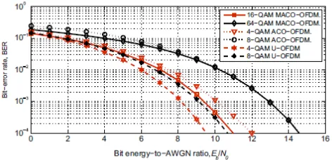
showing that both theoretical and simulations curves are in good agreement. Fig. 5 shows a BER comparison between ACO-OFDM, U-OFDM and MACO-OFDM at the same transmission data rate and receiver bandwidth. As shown in Eq. (24), in order to satisfy these constraints, the QAM level of ACO-OFDM and U-OFDM has to equal to the square root of that of MACO-OFDM. The BER comparisons are therefore made for a 4-QAM ACO-OFDM and 4-QAM U-OFDM to that of a 16-QAM MACO-OFDM and an QAM ACO-OFDM, 8-QAM U-OFDM to that of a 64-8-QAM MACO-OFDM. At a BER10
4, the proposed 16-QAM MACO-OFDM system has an energy saving of 1 dB when compared with traditional 4-QAM ACO-OFDM, wholly attributed to the sample averaging during unipolar decoding (Eq. (26)).Fig. 4. Bit-error rate of proposed MACO-OFDM system versus bit energy-to-AWGN ratio using both Monte Carlo simulation and theoretical analysis methods.
Fig. 5. Bit-error rate of the proposed MACO-OFDM, U-OFDM and traditional ACO-OFDM systems versus bit energy-to-AWGN ratio.
No saving in energy is evident when comparing 64-QAM MACO-OFDM with 8-QAM ACO-OFDM at this BER value. As expected the performance of MACO-OFDM decreases the gap between U-OFDM performance and ACO-OFDM.
5. MACO-OFDM TECHNIQUE IN ATMOSPHERIC TURBULENT CHANNELS
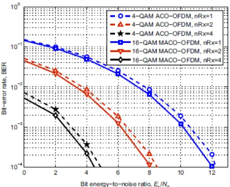
One of the most damaging impairments on Free Space Optical (FSO) system performance is atmospheric turbulence, induced irradiance fluctuations often referred to as scintillation [24]. Scintillation takes place as a result of heating of the surface of earth, resulting in the rise of thermal air masses. The masses combine forming regions with different densities and sizes, which cause differences in refractive indices varying with time. Moreover, these regions cause fluctuations in the irradiance of the received laser beam. A multiple-input multiple-output (MIMO) approach has been investigated as a solution, however in a dispersive channel, inter-symbol interference (ISI) is highly detrimental [24]. The use of OFDM in conjunction with MIMO technique has been suggested to overcome both ISI and the induced fading caused by atmospheric turbulence. MIMO-OFDM is currently used in the 4G wireless [25] and research has shown that deploying diversity at the receiver is more efficient than at the transmitter side [24]. A comparison of BER performance of both ACO-OFDM and MACO-ACO-OFDM techniques in turbulent channels using SIMO configurations is carried out.
5.1. Scintillation statistics and system model
[image:7.612.329.565.67.181.2] [image:7.612.56.286.510.691.2]demonstrated recently [24]. Throughout the analysis, the gamma–gamma channel model is adopted, the probability density function of which is the product of two in-dependent gamma random variables [26];
2 1
2
2(
)
( )
2
( ) ( )
f I
I
K
I
(44)where I is the signal intensity, Γ (·) is the gamma function,
K
is the modified Bessel function of the second kind of order α - β , and α and β are the effective positive parameters of the large- and small-scale eddies, respectively, that characterize irradiance fluctuation [24];
1 2
7/6 12/5
1 2
5/6 12/5
0.49
exp
1
1 1.11
0.51
exp
1
1 0.69
l l
l l
(45)
l
is the Rytov variance for plane wave, defined as [26];2
1.23
2 7/6 11/6l
C K
nL
(46) 2n
C
is the refractive-index structure parameter,k
2 /
/is the wave number, and L is the link length. The strength of atmospheric turbulence is represented by a factor known as scintillation index (SI), which depends on the Rytov variance [26];1 1
(
)
1SI
(47)5.2. Numerical results
[image:8.612.335.567.51.240.2]Monte Carlo simulations are carried out to investigate the BER performance of both ACO-OFDM and MACO-OFDM using MRC diversity at the receiver for
N
1, 2, 4
at different atmospheric conditions. As the SI value increases, so does the turbulence strength and the induced irradiance fluctuations. To keep the effective data rates of both systems identical, focus is set on 4-QAM ACO-OFDM and 16-QAM MACO-OFDM systems. Fig. 6 shows a BER comparison for weak turbulence (SI =0.11). [image:8.612.345.584.279.470.2]Fig. 6. BERs of both ACO-OFDM and MACO-OFDM systems versus the bit energy-to-noise ratio at = SI 0.11, α = 18.2530, and β = 16.5793.
Fig. 7. BERs of both ACO-OFDM and MACO-OFDM systems versus the bit energy-to-noise ratio at = SI 0.7, α = 4.3939, and β = 2.5636.
[image:8.612.344.582.527.713.2]As expected, the performances of both systems improve as the number of receiving photodetectors (nRx) increases. Specifically at a BER of
10
4, the performance of MACO-OFDM is better than that of ACO-MACO-OFDM by 0.5 dB for N= 1, 2, and 4. Fig. 7 shows the BER performance for moderate turbulence (increase of the SI to 0.7). The performance of both systems degrades, however MACO-OFDM still outperforms OFDM. The improvement of MOFDM over ACO-OFDM (at a BER of10
4) is 2.6 dB, 1 dB and 0.5 dB for N=1, N=2, and 4, respectively. For strong turbulence (SI=0.98), similar conclusions can be drawn (Fig. 8). However, the difference in the performance improvement increases; the improvement in performance becomes 4 dB, 2.2 dB and 0.5 dB at N= 1, N= 2 and 4, respectively.6. CONCLUSIONS
The adoption of unipolar encoding in ACO-OFDM has been proposed and the BER performance derived for the modified system. Monte Carlo simulations have been carried out to verify the analysis. In addition, the employment of the proposed system in the presence of atmospheric turbulence has been studied using single-input multiple-output (SIMO) configurations. Results have been compared to that of ACO-OFDM under same bit energy, transmission rate and receiver bandwidth. Energy improvements of about 4 dB and 2.2 dB can be noticed at a BER of
10
4with SIMO systems of 1 and 2 photodetectors, respectively, at the receiver for the case of strong turbulence.REFERENCES
[1] R.V. Nee, R. Prasad, OFDM for Wireless Multimedia Communications, Artech House, New York, 2000.
[2] H. Schuzle, C. Luders, Theory and Applications of OFDM and OCMA Wideband Wireless Communications, John Wiley, New York, 2008. [3] S. Glisic, Advanced Wireless Communications 4G Technologies, John
Wiley, New York, 2004.
[4] U. Madhow, Fundamentals of Digital Communications, Cambridge University Press, New York, 2008.
[5] J. Armstrong, OFDM for optical communications, J. Lightw. Technol. 27 (3) (2009) 189–204.
[6] Z. Ghassemlooy, W. Popoola, S. Rajbhandari, Optical Wireless Communications System and Channel Modelling with MATLAB, CRC Press, New York, 2013.
[7] L. Chen, B. Krongold, J. Evans, Performance evaluation of optical OFDM systems with nonlinear clipping distortion, in: IEEE International Conference on Communication (ICC 2009), Dresden, Germany, 2009, pp. 1–5.
[8] S. Dimitrov, S. Sinanovic, H. Haas, A comparison of OFDM- based modulation schemes for OWC with clipping distortion, in: IEEE Global Telecommunication Conference (GLOBECOM 2011), Houston, TX, 2011, pp. 787–791.
[9] S. Dimitrov, S. Sinanovic, H. Haas, Clipping noise in OFDM- based optical wireless communication systems, IEEE Trans. Commun. 60 (4) (2012) 1072–1081.
[10] J. Armstrong, B.J.C. Schmidt, Comparison of asymmetrically clipped optical OFDM and DC-biased optical OFDM in awgn, IEEE Commun. Lett. 12 (5) (2008) 343–345.
[11] L. Chen, B. Krongold, J. Evans, Diversity combining for asymmetrically clipped optical OFDM in IM/DD channels, in: IEEE Global Telecommunication Con- ference (GLOBECOM 2009), Honolulu, HI, 2009, pp. 1–6.
[12] S. D. Dissanayake, K. Panta, J. Armstrong, A novel technique to simultaneously transmit ACO-OFDM and DCO-OFDM in IM/DD systems, in: IEEE Global Telecommunication Conference (GLOBECOM 2011), Houston, TX, 2011, pp. 782–786.
[13] J. Armstrong, A. Lowery, Power efficient optical OFDM, Electron. Lett. 42 (6) (2006) 370–372.
[14] S.K. Wilson, J. Armstrong, Transmitter and receiver methods for improving asymmetrically- clipped optical OFDM, IEEE Trans. Wirel. Commun. 8 (9) (2009) 4561–4567.
[15] S. Dimitrov, S. Sinanovic, H. Haas, Double-sided signal clipping in ACO-OFDM wireless communication systems, in: IEEE International Conference on Com- munication (ICC 2009), Kyoto, Japan, 2009, pp. 1– 5.
[16] J. Armstrong, B.J. Schmidt, D. Karla, H.A. Suraweera, A.J. Lowery, Performance of asymmetrically clipped optical OFDM in AWGN for an intensity modulated direct detection system, in: IEEE Global Telecommunication Conference (GLOBECOM 2006), San Francisco, CA, 2006, pp. 1–5.
[17] D. Tsonev, S. Sinanovic, H. Haas, Novel unipolar orthogonal frequency division multiplexing (U-OFDM) for optical wireless, in: IEEE 75th Vehicular Technology Conference (VTC Spring 2012), Yokohama, Japan, 2012, pp. 1–5.
[18] W. Shieh, I. Djordjevic, OFDM for Optical Communications, Elsevier Press, New York, 2010.
[19] D. Dardari, V. Tralli, A. Vaccari, A theoretical characterization of nonlinear distortion effects in OFDM systems, IEEE Trans. Commun. 48 (10) (2000) 1755–1764.
[20] N. Fernando, Y. Hong, E. Viterbo, Flip-OFDM for optical wireless communications, in: Information Theory Workshop (ITW 2011), Paraty, Brazil, 2011, pp. 5–9. [21] S.D. Mohamed, I. Andonovic, H. Shalaby, M.H. Aly, Modified asymmetrically- clipped optical orthogonal frequency-division multiplexing system performance, in: IEEE Photonics Conference (IPC 2013), Bellevue, WA, 2013, pp. 289–290.
[22] S.D. Mohamed, H.S. Khallaf, H. Shalaby, I. Andonovic, M.H. Aly, Two approaches for the modified asymmetrically clipped optical orthogonal fre- quency division multiplexing system, in: Second International Japan– Egypt Conference on Electronics, Communications and Computers (JEC-ECC 2013), Cairo, Egypt, 2013, pp. 135–139.
[23] J. Lu, K.B. Letaief, J.C.-I. Chuang, M.L. Liou, M-PSK and M-QAM BER computa-tion using signal-space concepts, IEEE Trans. Commun. 47 (2) (1999) 181–184. [24] M. Mofidi, A. Chaman-motlagh, Error and channel capacity analysis of SIMO and MISO free-space optical communications, in: 20th Iranian Conference on Electrical Engineering (ICEE 2012), Tehran, Iran, 2012, pp. 1414–1418.
[25] M. Sharma, D. Chadha, V. Chandra, Capacity evaluation of MIMO-OFDM free space optical communication system, in: Annual IEEE India Conference (IN- DICON 2013), Mumbai, India, 2013, pp. 1–4.