Application of Heuristic Algorithms in Improving Performance of Soft Computing Models for Prediction of Min, Mean and Max Air Temperatures

Article

Application of Heuristic Algorithms in Improving

Performance of Soft Computing Models for Prediction

of Min, Mean and Max Air Temperatures

Armin Azad

_{, Jamshid Pirayesh}

_{, Saeed Farzin}

_{, Leila Malekani}

_,

Sheida Moradinasab

_{, and Ozgur Kisi}

1 Faculty of Civil Engineering, Semnan University, Semnan, Iran 2 Faculty of Electronic Engineering, Semnan University, Semnan, Iran 3 Faculty of Civil Engineering, University of Tabriz, Iran

4 Faculty of Chemistry, Semnan University, Semnan, Iran 5 School of Technology, Ilia State University, Tbilisi, Georgia

E-mail: a_{[email protected],} b_{[email protected],} c_{[email protected] (Corresponding} author), d_{[email protected],} e_{[email protected],} f_{[email protected]}

Abstract. Traditionally, climate conditions have been one of the influential factors in

population growth in worldwide. Hence, predicting these conditions can be an important step to improve life conditions in worldwide. In this study, application of genetic algorithm (GA) and particle swarm algorithm (PSO) were considered as alternatives to available algorithms for training artificial neural network (ANN) and adaptive neuro-fuzzy inference system (ANFIS) in order to predict air temperature. Therefore, monthly minimum, average and maximum air temperatures of Tehran-Iran station at 64-years (1951-2014) were selected as predicted time-series. First, the most appropriate inputs were selected for the models using sensitivity analysis. After that, long-term air temperatures (1 month, 1-, 2- and 3-year ahead) were modeled. Results showed that: 1) the given algorithms had acceptable results in improving the models’ performance in forecasting minimum, mean and maximum air temperatures. Also, they could improve the performance of ANN and ANFIS in most of the prediction intervals, 2) ANFIS-GA was selected as the most suitable model so that its average determination coefficient (R2_{), root mean square errors (RMSE) and mean absolute} errors (MAE) were 0.88, 1.41 and 2.52, respectively, 3) the sensitivity analysis provided suitable results in selecting the most appropriate model inputs for forecasting the minimum, mean and maximum air temperatures in different intervals.

Keywords: ANFIS, ANN, genetic algorithm, particle swarm algorithm, long-term air temperatures.

ENGINEERING JOURNAL Volume 23 Issue 6

1.

Introduction

Climate forecast is very important in agricultural water resources management, water supply and other daily issues. Climate temperature is also one of the most important input components for land evaluation models, hydrological and ecological models [1]. Some models were used to extract water evaporation, soil weathering and herbal product levels [2]. In other hand, climate temperature is applied as a critical feature to evaluate the fitness between crops and desired area [3], thereby suitable habitats with any plant species can be determined. To date, many studies has been conducted about the prediction of air temperature [4, 5, 6].

Among them, artificial intelligence models including artificial neural network (ANN) and adaptive neuro-fuzzy inference system (ANFIS) have shown suitable performance related to the prediction of different factors such as climate and environmental conditions due to the lack of physical perception of the issue [7, 8]. Smith et al. (2005) optimized ANN performance to model environment temperature using seasonal data. In another research, Ustaoglu et.al. (2008) estimated the minimum, mean and maximum daily air temperatures using time series inputs [9]. Dombaycı and Golcu (2009) predicted air temperature in southwest of Turkey using ANN model [10]. Abhishek et al. (2012) forecasted daily maximum temperature for each day of the year and concluded that variations in hidden layers and the number of neurons significantly affected model accuracy and over- fitting [11]. In another study, Daneshmand et.al. (2013) predicted monthly minimum temperature in Mashhad City, located in northeast of Iran, using ANNs and ANFIS models [12]. Results showed that the ANFIS had suitable performance. Kisi and Sanikhani (2015a), in another study, predicted air temperature in Iran stations using geographical data, in which support vector regression (SVR) model had the best performance in predicting temperature [13].

Although the performance of ANN and ANFIS can be categorized acceptable, they fail in some cases– especially when they try to forecast phenomena and not modeling them. In such a case, improving their ability seems to be necessary. Evolutionary algorithm (EA) is known as an appropriate way to cover the above-mentioned models. It is a way used as an alternative for classic training methods, mostly gradient based algorithms. In some cases that the results are not satisfying, by using EA methods, the model performance is improved as much as the results can be acceptable. The improvement roots in various advantages ANN and ANN combined with EA enjoy, as escaping from trapped in local optima, good ability in solving complex problems, using global searching method and so forth [14, 15].

In last years, scholars have focused on how EA response when it is used in improving ANN and ANFIS in modeling and predicting various environmental and hydrological phenomena, such as, river flow, water quality, rainfall, and so forth. Tabari (2016) reported Direct Search Optimization Algorithm (DSOA) as a suitable method to train fuzzy inference system (FIS) in order to predict river runoff. According to his study, DSOA had an acceptable performance in improving the FIS ability in predicting river runoff [16]. Kisi et al. (2017) modeled water level by an ANN combined with particle swarm optimization (PSO). The results showed the good performance of proposed method in estimating water level [17]. Azad et al. (2019) reported ant colony optimization (ACO) as an appropriate training algorithm alternative to standard ANFIS algorithm in modeling rainfall [8]. Kisi et al. (2019) proposed ANFIS combined with Genetic Algorithm as a good method to estimate groundwater quality parameters [18]. Azad et al. (2019) used four algorithms GA, PSO, ACO and differential evolution (DE) to train ANFIS in modeling air temperature. In a comprehensive study, they examined the suggested algorithm to estimate (not forecast) air temperature of 40 stations with various climatic conditions, arid, humid subtropical, hot and humid, and cold climate situations. According to them, ANFIS-GA had a very reliable performance such that the results were satisfying in 38 out of 40 modeled stations [19].

With respect to the studies, EAs, and especially PSO and GA, are reliable and accepted method to be utilized as alternative method to train soft computing models. According to the authors, application of GA and PSO algorithms in improving ANFIS and ANN performance to predict long-term (from 1 month ahead to 3 years ahead) minimum, mean and maximum air temperatures have not been studied before.

2.

Materials and Methods

2.1. Studied Region and Database

Tehran City as Iran capital is located in the south of Alborz mountains ranging with an area of over 20,000 km2 _{[14]. This city located in longitude and latitude of 51°19}́ and 35°_{41́ , respectively, and it has a height}

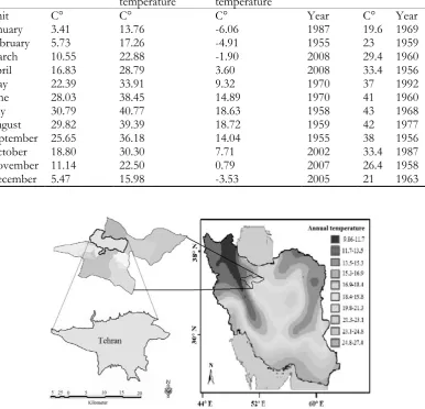
of 1190 meters above sea level and 17.4 ℃ average annual air temperature [15]. In this study, the extreme and mean temperatures data of studied region for the period 1951-2014 were captured from Iran Meteorological Organization (http://www.weather.ir). The geographical situation and data statistics related to studied region has been provided in Table 1 and Fig. 1. As seen from the table, the highest and lowest temperatures were observed for the July and January. The warmest (43 0_{C) and the coldest (-15} 0_C) temperatures were also measured in July of 1958 and in January of 1969, respectively.

Table 1. The statistic related to extremum temperature of Tehran in the period under study.

Coldest month’s day Warmest

month’s day

Min mean

monthly temperature

Max mean

monthly temperature Mean

temperature

C° Year C°

Year C°

C° C°

Unit

-15 1969 19.6 1987

-6.06 13.76

3.41 January

-13 1959 23

1955 -4.91

17.26 5.73

February

-8 1960 29.4 2008

-1.90 22.88

10.55 March

-4 1956 33.4 2008

3.60 28.79

16.83 April

2.4 1992 37

1970 9.32

33.91 22.39

May

5 1960 41

1970 14.89

38.45 28.03

June

14 1968 43

1958 18.63

40.77 30.79

July

13 1977 42

1959 18.72

39.39 29.82

August

9 1956 38

1955 14.04

36.18 25.65

September

2.8 1987 33.4 2002

7.71 30.30

18.80 October

-7 1958 26.4 2007

0.79 22.50

11.14 November

-13 1963 21

2005 -3.53

15.98 5.47

December

Fig. 1. Studied region situation.

2.2. Adaptive Neuro-Fuzzy Inference System (ANFIS)

models because of linguistic terms. Thus, their integration with neural network can be effective in solving complex and non-linear problems [22]. There are mainly two approaches for fuzzy inference systems, namely the approaches of Mamdani and Sugeno [23, 24]. It has many applications in controlling, predicting and different fields [25-28]. In order to prevent the manuscript to become voluminous, the classic ANFIS steps are not explained in the present study, and one can find them in the existing studies [6, 20, 24].

In this study, from 770 available data, 70% is dedicated for training and the remaining for testing section. It is notable that to escape over-fitting phenomena, the data were split randomly. Also, the best value of epoch number, initial step-size, step-size-decrease, and initial-increase were 500, 0.02, 0.8, and 1.2, respectively.

2.3. Artificial Neural Network (ANN)

The use of classic artificial neural network (ANN) that is inspired by human’s brain is capable of doing operations almost similar to neural systems but in the primary scale. The structure of network determines the number of neurons or processors element forming a network, the way they are placed and connected to each other. ANN starts with ban input layer and ends to an output layer. Several hidden layers can be found between these two layers. In these networks, the input information is lead to output layers after processing in neurons of hidden layer. Because of the volume limitations of the paper, the steps of classic ANN are not described here, and they can be found in the existing literature [15, 17].

It is notable, for classic ANN, that after trying various values, number of iterations, training algorithm, and type of the function were chosen 50000, gradient descent back-propagation (gd), Gaussian were selected.

2.4. Particle Swarm Optimization (PSO)

PSO was firstly proposed by Kendy and Eberhart (1995) [29]. PSO is one of the most widely used evolutionary algorithms based on population and has been used to solve many non-linear problems. The central conception of this algorithm was inspired from the comparison of biological and sociological behavior of organisms (birds, fishes etc.) [30]. Each solution is only a particle in research space in PSO. In the following, competence level of particle will be evaluated to optimize it by the algorithm. The algorithm pursues the suitable solution of each particle (the best local) and the suitable solution of total population (the best total) in each iteration. Total optimization will be provided as a final solution by the algorithm after termination of iteration. As same as previous sections, because the volume limitation, the algorithm steps are referred to the original studies [29, 30].

To establish the algorithms’ setting parameters for ANFIS-PSO, population size, personal and global best learning coefficients, inertia weight, and inertia weight reduction factor, max-iteration were fixed to 100, 1.9, 2.1, 1, 0.97, and 1200, respectively. Also, the mentioned parameters for ANN-PSO were, respectively, 75, 2, 2, 1.05, 0.98, and 10000. It is notable that these are the best and applied after trying various values.

2.5. Genetic Algorithm (GA)

GA is one of the most common algorithms to optimize system control parameters and also to solve non-linear and complex problems. It was proposed by Holland (1975) [31]. Its central component is chromosome. Each of chromosomes composed of gens which are the parameters of the problem. Problem-solving is started with an initial population. It continues with the rule of competence member survival and then compares this solution with other solutions. At last, criteria of optimization operation terminating are based on the number of chromosomes and generally the problem was terminated after production of certain numbers [32].

To determine the algorithm settings for ANFIS-GA, the best amounts of percent of mutation, population size, percent of crossover, and max-iteration, were 0.1, 65, 0.9, and 600, respectively; these parameters for ANN-GA were fixed to, respectively, 0.15, 70, 0.85, and 9000. It is notable that these are the best and applied after trying various values.

2.6. Models Structure

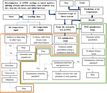
over-fitting and voluminous computations. Firstly, primary system structures (ratio of training and test stages etc.) are determined. Then, some parameters of the algorithm including iteration number, primary population of the algorithm, the ultimate value of optimization, the coefficients of some algorithms such as alpha and beta, target function and other parameters related to the algorithm are adjusted. It should be noted that data should be normalized. In the following, simple ANN and ANFIS are trained using new algorithms. The training procedure continues until the iteration numbers required reaches to end or achieve to goal error. At last, after training ANN and ANFIS, the processes continue like simple models and to the end of modeling.

Finally, its performance is tested using some statistic indices including determination coefficient (R2_), root mean square errors (RMSE) and mean absolute errors (MAE) etc. The performances of the ANFIS-GA and ANN-PSO models are provided in Figs. 2 and 3. It is noteworthy that the other simple ANN and ANFIS models also have similar structures and their difference are in the training stages of the algorithm. In this study, after employing various values, from 770 available data, 70% is dedicated randomly to training and the remaining to test section. The number of epochs in simple ANFIS and iteration, number, epoch of provided algorithms were set to 500. It is notable that the 500 is the optimal number of iterations for all models and higher number of the iterations has no considerable effect on models’ performance. In addition, as for the coefficients related to algorithms, their optimum values were obtained by trial and error and their most appropriate coefficients were used. In spite of algorithms settings, reported in sections 2.2 and 2.3, other parameters of suggested ANN and ANFIS are as same as ones used in classic models (Table 2 and 3).

Fig. 3. Steps of ANN-PSO and ANN-GA models

Table 2. Results of classic ANN training algorithms.

Training algorithm _structure Model Iteration _number

Levenberg–Marquardt back propagation (lm) 4-4-1 1500

Gradient descent back-propagation (gd) 4-2-1 50000

Gradient descent with adaptive learning rate backpropagation (gda) 4-4-1 50000 Gradient descent with momentum back propagation (gdm) 4-5-1 50000 Gradient descent with momentum and adaptive learning rate back-propagation (gdx) 4-4-1 50000 Scaled conjugate gradient back-propagation (scg) 4-5-1 2000

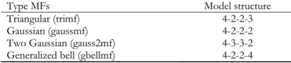
Table 3. Different simple ANFIS structures used.

Type MFs Model structure

Triangular (trimf) 4-2-2-3

Gaussian (gaussmf) 4-2-2-2

Two Gaussian (gauss2mf) 4-3-3-2

3.

Results and Discussion

3.1. Comparison Criteria

In this paper, the ANFIS, ANFIS-GA, ANFIS-PSO, ANN, ANN-GA and ANN-PSO were used to predict monthly minimum, average and maximum air temperatures of Tehran Station for the 63-year period (1951-2014) from 1 month to 3-years ahead. Therefore, first, the best inputs for each of time intervals (1month, 1, 2 and 3 years ahead) are specified using sensitivity analysis and then the temperatures are predicted. In the next step, for examining the ability of the applied algorithms for improving soft computing models (ANN and ANFIS), their performances are evaluated using R2_{, RMSE and MAE statistical indices. For the statistical} indices, the equations are provided in the following:









 



1 i

2 i n

1 i

2 i n

1 i

i i 2

y y x x y

y x x R

    

  

 

 









 



(1)







 

 n

1 i

2 i

i y

x n 1 RMSE

(2)

𝑀𝐴𝐸 = (|𝑥𝑖 − 𝑦𝑖

𝑛 |)

(3)

In these equations, xi and 𝑥̅ are observed values and their means and y and 𝑦̅ are predicted values and their means, respectively.

3.2. Sensitivity Analysis

The sensitivity analysis was used to select the best input data. It must be noted that all the results are not provided in this paper due to page limitations and also due to the desirable performances of the models in training stage.

3.2.1. Minimum temperature

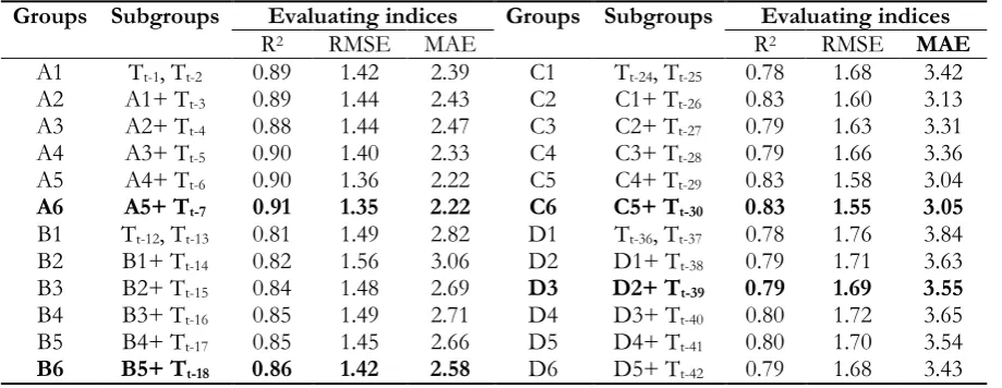
Data are split in four main groups (A, B, C, and D) to determine the best inputs to predict monthly minimum temperature of Tehran Station in four different time intervals. It is noteworthy that the given groups are related to the prediction of 1 month and 1, 2, and 3 years ahead temperatures, respectively. Also, each group is divided into six subgroups. Arrangements of subgroups are provided in Table 4. For example, the temperature with 12- and 13-month lags was allocated to the first subgroup (B1) to predict 1-year ahead temperature. In the increasing trend of subgroups (B2, B3, B4 …), temperature with monthly lags was added to previous subgroup at each time. So that, B6 had the lags from 12 to 18. Then, minimum temperature in each of time periods is estimated using available groups. The ANFIS-GA was used to predict them. It is notable that the model accuracy decreases by increasing time interval. In fact, the more the time interval increases, the harder the model works. In other words, when a model tries to predict a phenomena, it makes a relationship between input and output [14]. Therefore, by increasing the time interval, the model ability to make an accurate prediction is reduced, because making a true relationship between input and output become harder. It is one reason for EA suggestion; by using proposed EA methods, GA and PSO, the performance of ANN and ANFIS is improved in high time intervals, since the ability of GA and PSO is higher in making the true relation between the input and output compared to standard algorithms.

Table 4. Sensitive analysis for predicting minimum temperature. Evaluating indices Subgroups Groups Evaluating indices Subgroups Groups MAE RMSE R2 MAE RMSE R2 3.42 1.68 0.78 Tt-24, Tt-25 C1 2.39 1.42 0.89 Tt-1, Tt-2 A1 3.13 1.60 0.83 C1+ Tt-26 C2 2.43 1.44 0.89 A1+ Tt-3 A2 3.31 1.63 0.79 C2+ Tt-27 C3 2.47 1.44 0.88 A2+ Tt-4 A3 3.36 1.66 0.79 C3+ Tt-28 C4 2.33 1.40 0.90 A3+ Tt-5 A4 3.04 1.58 0.83 C4+ Tt-29 C5 2.22 1.36 0.90 A4+ Tt-6 A5 3.05 1.55 0.83 C5+ Tt-30

C6 2.22

1.35 0.91

A5+ Tt-7

A6 3.84 1.76 0.78 Tt-36, Tt-37 D1 2.82 1.49 0.81 Tt-12, Tt-13 B1 3.63 1.71 0.79 D1+ Tt-38 D2 3.06 1.56 0.82 B1+ Tt-14 B2 3.55 1.69 0.79 D2+ Tt-39

D3 2.69 1.48 0.84 B2+ Tt-15 B3 3.65 1.72 0.80 D3+ Tt-40 D4 2.71 1.49 0.85 B3+ Tt-16 B4 3.54 1.70 0.80 D4+ Tt-41 D5 2.66 1.45 0.85 B4+ Tt-17 B5 3.43 1.68 0.79 D5+ Tt-42 D6 2.58 1.42 0.86 B5+ Tt-18

B6

In 1 month ahead forecasting, A6 (Tt-1 to Tt-7 where Tt-1 indicates the monthly minimum temperature at one previous month) with R2_{, RMSE and MAE equal to 0.91, 1.35 and 2.22 provided the best accuracy.} B6 (Tt-12 to Tt-18) with the highest R2 _{(0.86) and the lowest errors (RMSE=1.42, MAE=2.58) was selected.} The determination coefficient and error indices were respectively decreased and increased in 2-year forecast horizon where the C6 with R2_{, RMSE and MAE equal to 0.83, 1.55 and 3.05, respectively, provided the best} performance. Finally, D3 was selected as the best inputs for the 3-year forecast horizon.

3.2.2. Mean temperature

To determine the best inputs for monthly mean air temperature using sensitive analysis. 4 groups including F, G, H, and I were arranged as reported in Table 3. Results showed that F4 (Tt-1 to Tt-3) was identified as the most appropriate group for predicting 1 month ahead temperature. For 1 year forecasting horizon, G2 was selected as the top option to forecast mean temperature in this time interval. In 2-year forecast horizon, H2 (Tt-26 to Tt-24) despite of RMSE equal to H1 (RMSEH1, H2=1.41), but due to more desirable R2 _{and MAE} (MAEH2=2.53, MAEH1=2.60, R2H2=0.86, R2H1) was selected as the most appropriate model. At last, I4 was the most appropriate model for 3-year forecasting interval. Comparison with Table 5 shows that the ANGIS-GA has better mean temperature forecasts compared to minimum temperatures. It should be noted that models’ ability in predicting air temperature is highly reduced with the increased forecasting horizon.

Table 5. Sensitivity analysis for predicting mean temperature.

Evaluating indices Subgroups Groups Evaluating indices Subgroups Groups MAE RMSE R2 MAE RMSE R2 2.60 1.41 0.85 Tt-24, Tt-25 H1 1.70 1.17 0.94 Tt-1, Tt-2 F1 2.53 1.41 0.86

H1+ Tt-26

H2 1.46 1.11 0.96 F1+ Tt-3 F2 2.81 1.50 0.85 H2+ Tt-27 H3 1.51 1.11 0.95 F2+ Tt-4 F3 3.45 1.69 0.79 H3+ Tt-28 H4 1.38 1.05 0.96 F3+ Tt-5

F4 2.82 1.51 0.85 H4+ Tt-29 H5 1.37 1.06 0.96 F4+ Tt-6 F5 2.63 1.44 0.86 H5+ Tt-30 H6 1.54 1.12 0.95 F5+ Tt-7 F6 3.47 1.67 0.79 Tt-36, Tt-37 I1 2.13 1.29 0.90 Tt-12, Tt-13 G1 3.27 1.61 0.82 I1+ Tt-38 I2 1.90 1.24 0.93 G1+ Tt-14

G2 3.50 1.70 0.78 I2+ Tt-39 I3 2.20 1.30 0.90 G2+ Tt-15 G3 2.99 1.55 0.83

I3+ Tt-40

3.2.3. Maximum temperature

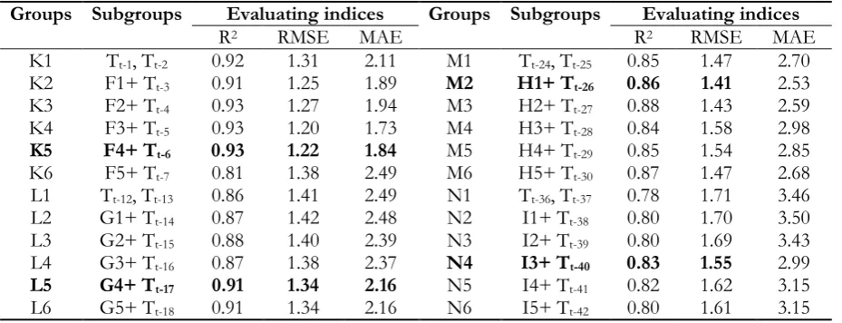
The sensitivity analysis in this section (Table 6) also had similar trend with two previous sections. According to the Table 4, K5 (Tt-1 to Tt-6) was identified as the most appropriate group in 1 month ahead forecasting. Next, L5 (Tt-12 to Tt-17) despite of its R2_{, RMSE and MAE equal to L6 (Tt-12 to Tt-18), but due to its lower} volume was selected as the most appropriate model for 1-year ahead forecasting. For 2-year time interval, M2 (Tt-24 to Tt-26) despite of its R2 _{lower than M3 (R2M2=0.86, R2M3=0.88), but due to its lower error and} volume was selected as the top model. At last, N4 (Tt-36 to Tt-40) was selected as the best input group to the model for forecasting 3-year ahead maximum temperatures. It must be noted that the difference between input performance in different time intervals and different temperatures can be attributed to the changes in the available data during the studied period. Also, it is noteworthy that in the sensitivity analysis, only 6 subgroups were provided for the minimum, mean and maximum air temperatures because more than this number did not produce better results.

Table 6. Sensitive analysis for predicting maximum temperature.

Evaluating indices Subgroups Groups Evaluating indices Subgroups Groups MAE RMSE R2 MAE RMSE R2 2.70 1.47 0.85 Tt-24, Tt-25 M1 2.11 1.31 0.92 Tt-1, Tt-2 K1 2.53 1.41 0.86

H1+ Tt-26

M2 1.89 1.25 0.91 F1+ Tt-3 K2 2.59 1.43 0.88 H2+ Tt-27 M3 1.94 1.27 0.93 F2+ Tt-4 K3 2.98 1.58 0.84 H3+ Tt-28 M4 1.73 1.20 0.93 F3+ Tt-5 K4 2.85 1.54 0.85 H4+ Tt-29 M5 1.84 1.22 0.93 F4+ Tt-6

K5 2.68 1.47 0.87 H5+ Tt-30 M6 2.49 1.38 0.81 F5+ Tt-7 K6 3.46 1.71 0.78 Tt-36, Tt-37 N1 2.49 1.41 0.86 Tt-12, Tt-13 L1 3.50 1.70 0.80 I1+ Tt-38 N2 2.48 1.42 0.87 G1+ Tt-14 L2 3.43 1.69 0.80 I2+ Tt-39 N3 2.39 1.40 0.88 G2+ Tt-15 L3 2.99 1.55 0.83

I3+ Tt-40

N4 2.37 1.38 0.87 G3+ Tt-16 L4 3.15 1.62 0.82 I4+ Tt-41 N5 2.16 1.34 0.91 G4+ Tt-17

L5 3.15 1.61 0.80 I5+ Tt-42 N6 2.16 1.34 0.91 G5+ Tt-18 L6

3.3. One Month Forecasting Horizon

After sensitivity analysis and identifying the most appropriate inputs to system, the six models (ANFIS, ANFIS-GA, ANFIS-PSO, ANN, ANN-GA and ANFIS-PSO) were used to predict the minimum, mean and maximum air temperatures of Tehran City in 1 month ahead. Ustaoglu et.al. (2008) reported that ANN models had desirable performance for the same time interval [9]. Daneshmand et al. (2013) also suggested that ANFIS had desirable performance in the prediction of daily minimum temperatures of Mashhad City located in the east of Iran [12]. Similar to the previous studies, in this study, also the artificial intelligence models provided desirable performance.

Table 7. Models performances in predicting one month ahead temperatures.

Tmax

Tmean

Tmin

Models _{R2 RMSE MAE R2 RMSE MAE R2 RMSE MAE}

2.04 1.31

0.91 1.93

1.26 0.90

2.04 1.31

0.91 ANFIS

1.73 1.20

0.93 1.38

1.05 0.96

2.22 1.35

0.91 ANFIS-GA

2.02 1.30

0.92 1.90

1.22 0.84

2.63 1.47

0.87 ANFIS-PSO

2.10 1.36

0.89 2.10

1.30 0.89

2.08 1.32

0.89 ANN

1.95 1.29

0.90 1.75

1.16 0.91

2.35 1.36

0.91 ANN-GA

2.02 1.32

0.89 1.97

1.28 0.89

2.72 1.52

0.90 ANN-PSO

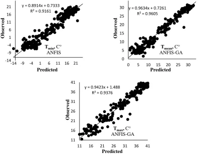
In consistent with the results of Ustaoglu et.al. (2008), soft computing models had suitable performance in the prediction of mean and maximum daily temperatures. It must be noted that the ANFIS-GA outperforms the ANFIS-PSO and this indicates that the GA has a higher ability in solving continuous problems [29]. It is notable that the input and output relationship has no much complexity in the short-term forecasting intervals such as 1 month. Therefore, ability of simple models is not completely tested for estimating climate temperature in such intervals and the models are not challenged as well. So, it is seen that the results of simple and hybrid models are very close to each other in such time period, even in some conditions, they outperformed the hybrid models. However, the performances of all hybrid models in this stage are generally better than the ANFIS and ANN. Scatterplots of the best models in forecasting minimum mean and maximum temperatures are illustrated in Fig. 4.

Fig. 4. Scatterplots of the best models in 1-month forecasting horizon.

3.4. One Year Forecasting Horizon

In this section, 1 year ahead air temperatures were predicted and results were given in Table 8. Generally, results showed that the most appropriate prediction belonged to maximum temperature while the weakest

y = 0.8914x + 0.7333 R² = 0.9161

-14 -9 -4 1 6 11 16 21

-14 -9 -4 1 6 11 16 21

O

bs

er

v

ed

Predicted T_min, C°

ANFIS

y = 0.9634x + 0.7261 R² = 0.9605

0 5 10 15 20 25 30

0 5 10 15 20 25 30

O

bs

er

v

ed

Predicted T_mean, C° ANFIS-GA

y = 0.9423x + 1.488 R² = 0.9376

11 16 21 26 31 36 41

11 16 21 26 31 36 41

O

bs

er

v

ed

prediction belonged to minimum temperature. The most suitable model to predict minimum temperature was related to ANFIS-GA and the weakest model was related to ANN. For the minimum temperatures, the accuracy ranks of the models are ANFIS-GA, ANN-GA, ANFIS, ANN-PSO, ANN and ANFIS-PSO. Same trend is also seen for the mean temperatures. Hybrid models related to GA (ANFIS-GA and ANN-GA) had the most appropriate performances and ANN showed the weakest performance.

Table 8. Models performance in predicting one year ahead temperatures.

Tmax

Tmean

Tmin

Models

MAE RMSE

R2 MAE

RMSE R2

MAE RMSE

R2

2.49 1.41

0.87 2.62

1.44 0.83

2.99 1.54

0.85 ANFIS

2.16 1.34

0.91 1.90

1.24 0.93

2.58 1.42

0.86 ANFIS-GA

2.37 1.38

0.89 2.59

1.40 0.85

3.20 1.63

0.81 ANFIS-PSO

2.55 1.45

0.80 2.66

1.47 0.79

3.26 1.62

0.78 ANN

2.25 1.33

0.89 2.55

1.30 0.85

2.75 1.50

0.84 ANN-GA

2.41 1.39

0.85 2.65

1.42 0.82

3.25 1.55

0.80 ANN-PSO

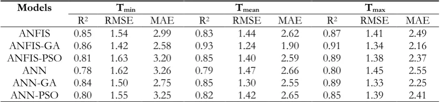
The model ANFIS-GA with the R2_{, RMSE and MAE equal to 0.91, 1.34 and 2.16 respectively, was} identified as the best model. The results showed high accuracy of the used models in the prediction of one year ahead Tmax Results also showed the ability of hybrid algorithms with ANFIS and ANN in improving the performance of these systems to predict 1 year ahead extreme temperatures of Tehran Station. The scatterplots of the best models in 1 year ahead temperatures were provided in Fig. 5. It is notable that the GA has more suitable performance than the PSO to improve ANN and ANFIS performances in predicting 1 year ahead temperatures. This suggests that the GA is a better alternative to existing algorithms of the ANN and ANFIS models.

3.5. Two-Year Forecasting Horizon

The models are compared in Table 7 for forecasting 2-year (24-month) ahead temperatures. Here, also the used models had suitable performance. The most accurate performance in the prediction of extreme and mean temperatures belonged to ANFIS-GA with the average R2_{, RMSE and MAE equal to 0.85, 1.62, and} 3.25, respectively and the weakest performance belonged to ANN with the average R2_{, RMSE and MAE} equal to 0.74, 1.74 and 3.44 respectively. The ANFIS-GA with the R2_{, RMSE and MAE equal to 0.83, 1.55} and 3.04 respectively was the most appropriate model in forecasting minimum temperatures in this time interval. After that, ANFIS-PSO, ANFIS, ANN-PSO, ANN-GA and ANN were ranked as the 2nd_{, 3}rd_{, 4}th_, 5th _{and 6}th_{, respectively. It is noteworthy that ANN-GA despite of its suitable performance in the previous} sections had no accurate results in this section, and it was as the 5th _{with the R}2 _{lower than the 0.81, RMSE} more than the 1.70 and MAE equal to 3.60 (Table 9).

Fig. 5. Scatterplots of the best models in 1-year forecasting horizon.

Table 9. Models performance in predicting 2-year ahead temperatures.

Tmax

Tmean

Tmin

Models

MAE RMSE

R2 MAE

RMSE R2

MAE RMSE

R2

3.28 1.63

0.82 2.92

1.54 0.85

3.55 1.69

0.80 ANFIS

2.53 1.41

0.86 2.53

1.41 0.86

3.04 1.55

0.83 ANFIS-GA

3.15 1.57

0.80 2.99

1.52 0.84

3.43 1.66

0.81 ANFIS-PSO

3.33 1.72

0.75 3.19

1.69 0.74

3.82 1.82

0.73 ANN

2.56 1.51

0.85 2.79

1.47 0.84

3.61 1.72

0.81 ANN-GA

3.25 1.65

0.82 2.99

1.52 0.81

3.45 1.73

0.80 ANN-PSO

y = 0.8772x + 0.9636 R² = 0.8601

-14 -9 -4 1 6 11 16 21

-14 -9 -4 1 6 11 16 21

O

bs

er

v

ed

Predicted T_min, C° ANFIS-GA

y = 0.9176x + 1.5432 R² = 0.9298

0 5 10 15 20 25 30

0 5 10 15 20 25 30

O

bs

er

v

ed

Predicted T_mean, C° ANFIS-GA

y = 0.9024x + 2.7106 R² = 0.9169

11 16 21 26 31 36 41

11 16 21 26 31 36 41

O

bs

er

v

ed

Predicted Tmax, C°

Fig. 6. Scatterplots of the best models in 2-year forecasting horizon.

3.6. Three-Year Forecasting Horizon

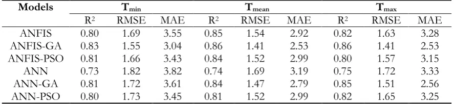
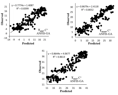
Table 10 compares the accuracies of the applied models in forecasting 3-year ahead minimum, mean and maximum temperatures. The hybrid models had suitable performance in improving ANFIS and ANN to estimate the minimum temperature in this time interval so that the mean performance of the hybrid models had R2_{, RMSE and MAE equal to 0.79, 1.66, and 3.61, respectively. On the other hand, averagely, GA had} the best results in the prediction of extreme and mean temperatures similar to the previous application. It is noteworthy that the GA had better performance than the PSO in training simple models. Also, it is noteworthy that the GA algorithm trains the ANN and ANFIS models better than the PSO at the most predicting intervals [1, 8, 15]. Therefore, GA is selected as the most acceptable alternative for training ANN and ANFIS in forecasting air temperatures. Figure 7 shows the best models’ performances for the 3-year forecasting horizon.

4.

Conclusions

Air temperature is one of the most important effective factors in the human life. This study had three overall conclusions which could be briefly addressed as: 1) Soft computing models applied in the current study had suitable performance in prediction of long-term extreme and mean temperatures, 2) The proposed hybrid models (ANFIS-PSO, ANFIS-GA, ANN-GA and ANN-PSO) provided good accuracy in the optimization of ANFIS and ANN. ANFIS-GA was the most accurate model. Also, by increasing prediction horizon to 2 and 3-year ahead, the performance of ANFIS-GA was decreased less than the other models, 3) Using the sensitivity analysis, the optimal inputs were determined in predicting long-term air temperatures for each of the time intervals. Such that in some of the groups, R2_{, RMSE and MAE were improved by 0.07, 0.28 and}

y = 0.7774x + 1.4087 R² = 0.8399

-14 -9 -4 1 6 11 16 21

-14 -9 -4 1 6 11 16 21

O

bs

er

v

ed

Predicted

Tmin, C°

ANFIS-GA

y = 0.8679x + 2.4118 R² = 0.8652

0 5 10 15 20 25 30

0 5 10 15 20 25 30

O

bs

er

v

ed

Predicted T_mean, C° ANFIS-GA

y = 0.8644x + 4.0677 R² = 0.8613

11 16 21 26 31 36 41

11 16 21 26 31 36 41

O

bs

er

v

ed

0.36, respectively. Finally, GA was selected as the most suitable algorithm for improving the performance of ANN and ANFIS in prediction of minimum, mean and maximum air temperatures.

Finally, to develop this study, 2 directions are suggested: (1) Both PSO and GA are well-known algorithms used in many different areas and had acceptable performance; however, using some new methods and combining them with ANN and ANFIS as well as compare their performance with the models proposed in this study can be as a measurement for their performance; (2) Using PSO and GA in order to improve performance of other popular soft computing models, such as SVR, decision tree, GPE, and etc.; (3) Using the suggested models to model air temperature in other locations of the world with different climate conditions.

Fig. 7. Scatterplots of the best models in 3-year forecasting horizon.

Table 10. Models performance in predicting 3-year ahead temperatures.

Tmax

Tmean

Tmin

Models

MAE RMSE

R2 MAE

RMSE R2

MAE RMSE

R2

3.50 1.69

0.75 3.24

1.59 0.79

4.34 1.89

0.75 ANFIS

2.99 1.55

0.83 2.99

1.55 0.83

3.43 1.68

0.82 ANFIS-GA

3.50 1.66

0.77 3.12

159 0.80

3.65 1.85

0.80 ANFIS-PSO

4.20 2.02

0.65 4.12

1.98 0.66

4.87 2.23

0.63 ANN

3.09 1.60

0.79 3.06

1.55 0.81

3.55 1.73

0.80 ANN-GA

6.52 1.66

0.73 3.20

1.62 0.79

4.30 1.90

0.76 ANN-PSO

y = 0.7774x + 1.4087 R² = 0.8299

-14 -9 -4 1 6 11 16 21

-14 -9 -4 1 6 11 16 21

O

bs

er

v

ed

Predicted T_min, C° ANFIS-GA

y = 0.7985x + 3.8319 R² = 0.8303

0 5 10 15 20 25 30

0 5 10 15 20 25 30

O

bs

er

v

ed

Predicted

T_mean, C° ANFIS-GA

y = 0.8574x + 4.0452 R² = 0.8319

11 16 21 26 31 36 41

11 16 21 26 31 36 41

O

bs

er

v

ed

Reference

[1] A. Azad, S. Farzin, H. Kashi, H.Sanikhani, H. Karami, and O. Kisi, “Prediction of river flow using hybrid neuro-fuzzy models,” Arabian Journal of Geosciences, vol. 11, pp. 718, 2018.

[2] R. Dodson and D. Marks, “Daily air temperature interpolated at high spatial resolution over a large mountainous region,” Climate Research, vol. 8, no, 1, pp. 1-20, 1997.

[3] G. Hudson and H. Wackernagel, “Mapping temperature using kriging with external drift: Theory and an example from Scotland,” International Journal of Climatology, vol. 14, pp. 77-91, 1994.

[4] A. Király and I. M. Jánosi, “Stochastic modeling of daily temperature fluctuations,” Physical Review, vol. 65, p. 051102, 2002.

[5] J. C. Aznar, E. Gloaguen, D. Tapsoba, S. Hachem, D. Caya, and Y. Bégin, “Interpolation of monthly mean temperatures using cokriging in spherical coordinates,” International Journal of Climatology, vol. 33, pp. 758-769, 2013.

[6] Z. A. Holden, M. A. Crimmins, S. A. Cushman, and J. S. Littell, “Empirical modeling of spatial and temporal variation in warm season nocturnal air temperatures in two North Idaho mountain ranges, USA,” Agricultural and Forest Meteorology, vol. 151, pp. 261-269, 2011.

[7] P. Kittisupakorn, P. Somsong, M. A. Hussain, and W. Daosud, “Improving of crystal size distribution control based on neural network-based hybrid model for purified terephthalic acid batch crystallizer,”

Engineering Journal, vol. 21, pp. 319-331, 2017.

[8] A. Azad, M. Manoochehri, H. Kashi, S. Farzin, H. Karami, V. Nourani, and J. Shiri, “Comparative evaluation of intelligent algorithms to improve adaptive neuro-fuzzy inference system performance in precipitation modelling,” Journal of Hydrology, vol. 571, pp. 214-224, 2019.

[9] B. Ustaoglu, H. K. Cigizoglu, and M. Karaca, “Forecast of daily mean, maximum and minimum temperature time series by three artificial neural network methods,” Meteorological Applications, vol. 15, pp. 431-445, 2008.

[10] O. A. Dombaycı, and M. Gölcü, “Daily means ambient temperature prediction using artificial neural network method: A case study of Turkey,” Renewable Energy, vol. 34, pp. 1158-1161, 2009.

[11] K. Abhishek, M. P. Singh, S. Ghosh, and A. Anand, “Weather forecasting model using artificial neural network,” Procedia Technology, vol. 4, pp. 311-318, 2012.

[12] H. Daneshmand, T. Tavousi, M. Khosravi, and S. Tavakoli, “Modeling minimum temperature using Adaptive Neuro-Fuzzy Inference System based on spectral analysis of climate indices: A case study in Iran,” Journal of the Saudi Society of Agricultural Sciences, vol. 14, pp. 33-40, 2015.

[13] O. Kisi and H. Sanikhani, “Modelling long‐term monthly temperatures by several data‐driven methods using geographical inputs,” International Journal of Climatology, vol. 35, pp. 3834-3846, 2015.

[14] A. Azad, H. Karami, S. Farzin, S-F. Mousavi, and O. Kisi, “Modeling river water quality parameters using modified adaptive neuro fuzzy inference system,” Water Science and Engineering, vol. 12, pp. 45-54, 2019.

[15] K. V. Shihabudheen and G. N. Pillai, “Recent advances in neuro-fuzzy system: A survey,”

Knowledge-Based Systems, vol. 152, pp. 136-162, 2018.

[16] M. M. R. Tabari, “Prediction of river runoff using fuzzy theory and direct search optimization algorithm coupled model,” Arabian Journal for Science and Engineering, vol. 41, pp. 4039-4051, 2016.

[17] O. Kisi, J. Shiri, and V. Demir, “Hydrological time series forecasting using three different heuristic regression techniques,” in Handbook of Neural Computation. Academic Press, 2017, pp. 45-65.

[18] O. Kisi, A. Azad, H. Kashi, A. Saeedian, S. A. A. Hashemi, and S. Ghorbani, “Modeling groundwater quality parameters using hybrid neuro-fuzzy methods,” Water Resources Management, vol. 33, pp.847-861, 2019.

[19] A. Azad, H. Kashi, S. Farzin, V. P. Singh, O. Kisi, H. Karami, and H. Sanikhani, “Novel approaches for air temperature prediction: Comparison of four hybrid evolutionary fuzzy models,” Meteorological Applications, 2019, to be published. [Online]. https://doi.org/10.1002/met.1817.

[20] J. S. Jang, “ANFIS: Adaptive-network-based fuzzy inference system,” IEEE Transactions on Systems, Man,

and Cybernetics, vol. 23, pp. 665-685, 1993.

[22] J. S. R. Jang, C. T. Sun, and E. Mizutani, “Neuro-fuzzy and soft computing: a computational approach to learning and machine intelligence,” IEEE Transactions on Automatic Control, vol. 42, no. 10, pp. 1482-1484, 1997.

[23] E. H. Mamdani, and S. Assilian, “An experiment in linguistic synthesis with a fuzzy logic controller,”

International Journal of Man-Machine Studies, vol. 7, pp. 1-13, 1975.

[24] T. Takagi, T. and Sugeno, M. “Fuzzy identification of systems and its applications to modeling and control,” IEEE Transactions on Systems, Man, and Cybernetics, vol. 1, pp.116-132, 1985.

[25] P. Kittisupakorn, P. Somsong, M. A. Hussain, and W. Daosud. “Improving of crystal size distribution control based on neural network-based hybrid model for purified terephthalic acid batch crystallizer,”

Engineering Journal, vol. 21, pp. 319-331, 2017.

[26] W. Daosud, J. Thampasato, and P. Kittisupakorn, “Neural network based modeling and control for a batch heating/cooling evaporative crystallization process,” Engineering Journal, Vol. 21, pp. 127-144, 2017.

[27] P. G. Rao, P. S. Rao, and B. B. V. L. Deepak, “GRNN-immune based strategy for estimating and optimizing the vibratory assisted welding parameters to produce quality welded joints,” Engineering

Journal, vol. 21, pp. 251-267, 2017.

[28] P. Samui and D. P. Kothari, “A multivariate adaptive regression spline approach for prediction of maximum shear modulus and minimum damping ratio,” Engineering Journal, vol. 16, pp. 69-78, 2012. [29] J. Kennedy and R. Eberhart, “Particle swarm optimization,” in Proceedings of the IEEE International

Conference on Neural Networks, 1955, vol. 4, pp. 1942-1948.

[30] Z. A. Bashir and M. E. El-Hawary, “Applying wavelets to short-term load forecasting using PSO-based neural networks,” IEEE Transactions on Power Systems, vol. 24, pp. 20-27, 2009.

[31] J. H. Holland, Adaptation in Natural and Artificial Systems: An Introductory Analysis with Applications to Biology,

Control, and Artificial Intelligence. MIT Press, 1992.