White Rose Research Online URL for this paper:
http://eprints.whiterose.ac.uk/787/
Article:
Billings, S.A. and Wei, H.L. (2005) A new class of wavelet networks for nonlinear system
identification. IEEE Transactions on Neural Networks, 16 (4). pp. 862-874. ISSN
1045-9227
https://doi.org/10.1109/TNN.2005.849842
[email protected] https://eprints.whiterose.ac.uk/
Reuse
Unless indicated otherwise, fulltext items are protected by copyright with all rights reserved. The copyright exception in section 29 of the Copyright, Designs and Patents Act 1988 allows the making of a single copy solely for the purpose of non-commercial research or private study within the limits of fair dealing. The publisher or other rights-holder may allow further reproduction and re-use of this version - refer to the White Rose Research Online record for this item. Where records identify the publisher as the copyright holder, users can verify any specific terms of use on the publisher’s website.
Takedown
If you consider content in White Rose Research Online to be in breach of UK law, please notify us by
A New Class of Wavelet Networks for Nonlinear
System Identification
Stephen A. Billings and Hua-Liang Wei
Abstract—A new class of wavelet networks (WNs) is proposed for nonlinear system identification. In the new networks, the model structure for a high-dimensional system is chosen to be a superimposition of a number of functions with fewer variables. By expanding each function using truncated wavelet decomposi-tions, the multivariate nonlinear networks can be converted into linear-in-the-parameter regressions, which can be solved using least-squares type methods. An efficient model term selection approach based upon a forward orthogonal least squares (OLS) algorithm and the error reduction ratio (ERR) is applied to solve the linear-in-the-parameters problem in the present study. The main advantage of the new WN is that it exploits the attractive features of multiscale wavelet decompositions and the capability of traditional neural networks. By adopting the analysis of variance (ANOVA) expansion, WNs can now handle nonlinear identifica-tion problems in high dimensions.
Index Terms—Nonlinear autoregressive with exogenous inputs (NARX) models, nonlinear system identification, orthogonal least squares (OLS), wavelet networks (WNs).
I. INTRODUCTION
W
AVELET theory [1]–[3] has been extensively studied in recent years and has been widely applied in various areas throughout science and engineering. Dynamical system mod-eling and control using artificial neural networks (ANNs), in-cluding radial basis function networks (RBFNs), has also been studied widely and a number of systematic approaches have been proposed [4]–[16]. The idea of combining wavelets with neural networks has led to the development of wavelet networks (WNs), where wavelets were introduced as activation functions of the hidden neurons in traditional feedforward neural networks with a linear output neuron. Although it was considered that WNs were popularized by the work in [17]–[19], the origin of WNs can be traced back to the earlier work of Daugman [20], where Gabor wavelets were used for image classification and compression.The wavelet analysis procedure is implemented with dilated and translated versions of a mother wavelet. Since signals of interest can usually be expressed using wavelet decompositions, signal processing algorithms can be performed by adjusting only the corresponding wavelet coefficients. In theory, the dilation (scale) parameter of a wavelet can be any positive real
Manuscript received March 22, 2004; October 26, 2004. This work was supported in part by the Engineering and Physical Sciences Research Council (EPSRC) (U.K.).
The authors are with the Department of Automatic Control and Sys-tems Engineering, University of Sheffield, Sheffield S1 3JD, U.K. (e-mail: [email protected]; [email protected]).
Digital Object Identifier 10.1109/TNN.2005.849842
value and the translation (shift) can be an arbitrary real number. This is referred to as the continuous wavelet transform. In practice, however, in order to improve computation efficiency, the values of the shift and scale parameters are often limited to some discrete lattices. This is then referred to as the discrete wavelet transform.
Both continuous and discrete wavelet transforms have been introduced to implement neural networks. Existing WNs can, therefore, be catalogued into the following two types.
• Adaptive WNs, where wavelets as activation functions stem from the continuous wavelet transform and the un-known parameters of the networks include the weighting coefficients (the outer parameters of the network) and the dilation and translation factors of the wavelets (the inner parameters of the network). These parameters can be viewed as coefficients varying continuously as in con-ventional neural networks and can be learned by gradient type algorithms.
• Fixed grid WNs, where the activation functions stem from the discrete wavelet transforms and unlike in adaptive neural networks, the unknown inner parameters of the networks vary on some fixed discrete lattices. In such a WN, the positions and dilations of the wavelets are fixed (predetermined) and only the weights have to be optimized by training the network. In general, gradient type algorithms are not needed to train such a network. An alternative solution for training this kind of network is to convert the networks into a linear-in-the-parameters problem, which can then be solved using least squares type algorithms.
The concept of adaptive WNs was introduced in [18] as an approximation route which combined the mathematical rigor of wavelets with the adaptive learning scheme of conventional neural networks into a single unit. Adaptive WNs have been successfully applied to nonlinear static function approxima-tion and classificaapproxima-tion [17], [21]–[24], and dynamical system modeling [25], [26]. Clearly, to train an adaptive WN, the gradients with respect to all the unknown parameters have to be expressed explicitly. The calculation of gradients may be heavy and complicated in some cases especially for high-di-mensional models. In addition, most gradient type algorithms are sensitive to initial conditions, that is, the initialization of wavelet neural networks is extremely important to obtain a fast convergence for a given algorithm [27]. Another problem that needs to be considered for training an adaptive WN is how to determine the initial number of wavelets associated with the network. These drawbacks often limit the application of
adaptive WNs to low dimensions for dynamical identification problems.
Unlike adaptive WNs, in a fixed grid WN, the number of wavelets as well as the scale and translation parameters can be determined in advance. The only unknown parameters are the weighting coefficients, that is, the outer parameters, of the network. The WN is now a linear-in-the-parameters regression, which can then be solved using least squares techniques. As will be discussed in Section III-D, the number of candidate wavelet terms in a fixed grid WN often increases dramatically with the model order. As a consequence, fixed grid WNs are often lim-ited to low dimensions.
Inspired by the well-known analysis of variance (ANOVA) expansions [28], [29], a new class of fixed grid WNs is intro-duced in the present study for nonlinear system identification. In the new WNs, the model structure of a high-dimensional system is initially expressed as a superimposition of a number of functions with fewer variables. By expanding each func-tion using truncated wavelet decomposifunc-tions, the multivariate nonlinear networks can then be converted into linear-in-the-pa-rameter problems, which can be solved using least-squares type methods. The new WNs are, therefore, in structure different from either the existing WNs [18], [24]–[26], [30]–[32] or wavelet mutiresolution models [33], [34]. A wavelet multires-olution model is in structure similar to a fixed grid WN. The former, however, forms a wavelet multiresolution decompo-sition similar to an ordinary multiresolution analysis (MAR), which involves not only a wavelet, but also another function, the associatedscaling function, where some additional require-ments should be satisfied. An efficient model term detection approach based on a forward orthogonal least squares (OLS) algorithm, along with the error reduction ratio (ERR) crite-rion [35]–[37] is applied to solve the linear-in-the-parameters problem in the present study.
II. PRESENTATION OFNONLINEARDYNAMICALSYSTEMS
A wide range of nonlinear systems can be represented using the nonlinear autoregressive with exogenous inputs (NARX) model. Taking single-input–single-output (SISO) systems as an example, this can be expressed by the following nonlinear dif-ference equation:
(1)
where is an unknown nonlinear mapping, and are the sampled input and output sequences, and are the max-imum input and output lags, respectively. The noise variable is immeasurable but is assumed to be bounded and uncorrelated with the inputs.
Several approaches can be applied to realize the represen-tation (1) including polynomials [36], [41], [42], neural net-works [4]–[6], [8] and other complex models [43]. In the present study, an additive model structure will be adopted to represent the NARX model (1). The multivariate nonlinear function in
the model (1) can be decomposed into a number of functional components via the well-known functional ANOVA expansions [28], [29]
(2)
where and
. (3) The first functional component is a constant to indicate the intrinsic varying trend; , are univariate, bivariate, etc., functional components. The univariate functional components represent the independent contribution to the system output that arises from the action of the th variable alone; the bivariate functional components represent the interacting contribution to the system output from the input vari-ables and , etc. The ANOVA expansion (2) can be viewed as a special form of the NARX model for input and output dynamical systems. Although the ANOVA decomposition of the NARX model (1) involves up to different functional components, experience shows that a truncated representation containing the components up to the bivariate or tri-variate functional terms often provides a satisfactory description of for many high dimensional problems providing that the input variables are properly selected [44], [45]. It is obvious that adopting a truncated ANOVA expansion containing only low-dimensional function components does not mean such an approach will always be appropriate. An exhaustive search for all the possible submodel structures of (2) is demanding and can be prohibitive because of the curse-of-dimensionality. A truncated representation is advantageous and practical if the higher order terms can be ignored. Note that the function does not contain terms that can be written as functional components with an order smaller than . It was also assumed that each functional component of the desired ANOVA expansion is square-integrable over the domain of interest for given data sets. In practice, the constant term can often set to be zero. If the constant term is different from zero for a given system, it can then be approximated by a wavelet expansion providing that the approximation is restricted to a compact subset of .
model type, are an important part of the nonlinear autoregres-sive moving average with exogenous inputs (NARMAX) mod-eling methodology [9]. If the model is adequate to represent the system the residuals should be unpredictable from all linear and nonlinear combinations of past inputs and outputs. This means that the identified model has captured all the predictable infor-mation in the data and is, therefore, the best that can be achieved by any model. It is, therefore, perfectly acceptable to fit a model that includes just bivariate or trivariate terms initially. The model validity tests should then be applied to test if the model that is obtained has captured all the predictable information in the data. If the model fails the model validity tests higher order terms should be included in the initial search set and the procedure should be repeated. It is, therefore, not necessary to prove that it is always possible to proceed based on just bi- and tri-variate terms. The identification proceeds a stage at a time and uses model validation as the decision making process. This is the NARMAX methodology [9], which is implemented here, and which mimics the traditional approach to analytical modeling. In the latter case, the most important model terms are included in the model initially then the less significant terms are added until the model is considered to be adequate. This is exactly what the OLS algorithm and the ERR does but based on the data. The most significant model terms are added first, step by step, a term at a time. The ERR cutoff value is used as a stopping mechanism but the model should never be accepted without applying model validity tests. If these tests fail go back and either reduce the ERR cutoff, or allow more complex model terms in the initial model library, or both and continue until the model validity tests are satisfied.
In practice, many types of functions, such as kernel func-tions, splines, polynomials and other basis functions [46] can be chosen to express the functional components in model (2). It is known that wavelet basis functions have the property of local-ization in both time and frequency. With the excellent approx-imation properties associated with multiscale decompositions, wavelet models outperform many other approximation schemes and are well-suited for approximating arbitrary functions [1], even functions with sharp discontinuities. It has been shown that the intrinsic nonlinear dynamics related to real nonlinear sys-tems can easily be captured by an appropriately fitted wavelet model consisting of a small number of wavelet basis functions [31], [34], and this makes wavelet representations more adap-tive compared with other basis functions. In the present study, therefore, wavelet decompositions, which are discussed in the next section, will be chosen to describe the functional compo-nents in the additive models (2), and this was referred to as the wavelet-NARX model, or the WANARX [45], where multires-olution wavelet decompositions were employed and a class of compactly supported wavelets was considered.
III. WNsANDTRUNCATEDWAVELETDECOMPOSITIONS
This section briefly reviews some results on wavelet decom-positions and WNs which are relevant to the present work. For more details about these results, see [1]–[3], [18], [31], [47], and [48]. In the following, it is assumed that the independent vari-able of a function of interest is defined in the unit
interval . In addition, for the sake of simplicity, one-dimen-sional (1-D) wavelets are considered as an example to illustrate related concepts.
A. Wavelet Decompositions
Let be a mother wavelet and assume that there exists a denumerable family derived from
(4)
where and are the scale and translation parameters. The normalization factor is introduced so that the energy of is preserved to be the same as that of . Rearrange the elements of so that
(5)
where is an index set which might be finite or infinite. Note that the double index of the elements of in (4) is replaced by a single index as shown in (5). Under the condition that generates a frame, it is guaranteed that any function
can be expanded in terms of the elements in in the sense that [1], [2], [18]
(6)
(7)
where are the decomposition coefficients or weights. Equa-tion (7) is called thewavelet frame decomposition.
In practical applications the decomposition (7) is often dis-cretized for computational efficiency by constricting both the scale and dilation parameters to some fixed lattices. In this way, wavelet decompositions can be obtained to provide an alterna-tive basis function representation. The most popular approach to discetize (7) is to restrict the dilation and translation parameters
to a dyadic lattice as and with (
is the set of all integers). Other nondyadic ways of discretization are also available. For the dyadic lattice case, (7) becomes
(8)
where and .
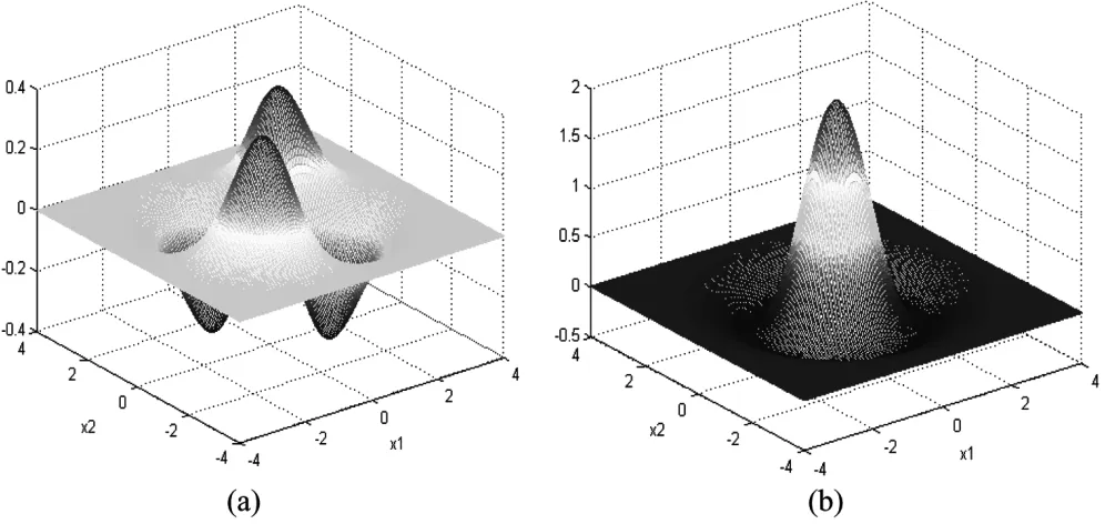
Fig. 1. Two-dimensional Gaussian and Marr mother wavelets. (a) Gaussian wavelet. (b) Marr wavelet.
functions is given to a wavelet frame by relaxing the orthogo-nality.B.
B. WNs
In practical applications for either static function learning or dynamical system modeling, it is unnecessary and impossible to represent a signal using an infinite decomposition of the form (7) or (8) in terms of wavelet basis functions. The decomposi-tions (7) and (8) are therefore often truncated at an appropriate accuracy. WNs are in effect nothing but a truncated wavelet de-composition. Taking the decomposition (8) as an example, an approximation to a function using the truncated wavelet decomposition with the coarsest resolution and the finest resolution can be expressed in the following:
(9)
where are subsets of and often
depend on the resolution level for all compactly supported wavelets and for most rapidly vanishing wavelets that are not compactly supported. The details on how to determine at a given level will be discussed later. Define
(10)
Assume that the number of wavelets in is . For con-venience of description, rearrange the elements of so that the double index can be indicated by a single index
in the sense that
(11)
The truncated wavelet decompositions (9) and (11) are re-ferred to asfixed grid WNs, which can be implemented using
neural network schemes by choosing different types of wavelets and employing different training/learning algorithms. This will be discussed in Section IV.
Note that although the WN (9) or (11) involves different res-olutions or scales, it cannot be called a multiresolution decom-position related to wavelet MAR, which involves not only a wavelet, but also another function, the associatedscaling func-tion, where some additional requirements should be satisfied.
C. Extending to High Dimensions
The results for the 1-D case described previously can be ex-tended to high dimensions. One commonly used approach is to generate separable wavelets by the tensor product of several 1-D wavelet functions. For example, an -dimensional wavelet can be constructed using a scalar wavelet as follows:
(12)
Another popular scheme is to choose the wavelets to be some radial functions. For example, the -dimensional Gaussian type functions can be constructed as
(13)
where . Similarly, the -dimensional
Mexican hat (also called the Marr) wavelet can be expressed as . In the present study, the radial wavelets are used to implement WNs. The two-dimen-sional (2-D) Gaussian and Mexican hat wavelets are shown in Fig. 1.
D. Limitations of Existing WNs
of the so calledcurse-of-dimensionality. The following discus-sion will illustrate why existing WNs are not readily suitable for high-dimensional problems.
Assume that a function of interest is defined in the unit hypercube . Let be a scalar wavelet function that is compactly supported on . From Section III-C, this scalar wavelet can be used to generate an -dimensional wavelet
by (12). This multidimensional wavelet can then be used to approximate the -dimensional function
using the WN (9) in the following:
(14)
where is an -dimensional index.
Noting that for and that the wavelet
is compactly supported on . Then for a given reso-lution level , it can easily be proved that the possible values
for should be between and , that is,
. Therefore, the number of candidate wavelet terms to be considered at scale level will
be , where . Setting 5
and 5, this number will be , , , and
for 0,1,2, and 3, respectively. If and are set to be 10 and 5, the number of candidate wavelets will then
become , , , and for 0,1,2, and
3, respectively. This implies that the total number of candidate wavelet terms involved in the WN can become very large even for some low resolution levels . This means that the computation task for a medium or high-dimensional WN can become very high. Thus, it can be concluded that high-dimen-sional WNs will be very difficult if not impossible to imple-ment via a tensor product approach. This is the case where an -dimensional wavelet is constructed by the tensor product of
scalar wavelets.
Similarly, applications of existing WNs, where the wavelets are chosen to be radial wavelets, are also prohibited from high-dimensional problems by the previously mentioned limitations. In addition, most existing radial WNs possess an inherent draw-back, that is, every wavelet term includes all the process vari-ables as in the Gaussian and the Marr mother wavelets. This is unreasonable since in general it is not necessary that every variable of a process interacts directly with all the other vari-ables. Moreover, experience shows that inclusion of the total-variable-involvedwavelet terms (here atotal-variable-involved term refers to a model term that involves all the process vari-ables simultaneously) may produce a deleterious effect on the resulting model of a dynamical process and will often induce spurious dynamics. From the point of view of identification studies, it is therefore desirable to exclude the total-variable-in-volved wavelet terms.
The limitations and drawbacks associated with existing WNs described previously suggest that new WNs need to be con-structed to bypass the curse-of-dimensionality to enable the net-works to handle more realistic and high-dimensional problems.
IV. NEWCLASS OFWNs
The structure of the new WNs is based on the ANOVA expan-sion (2), where it is assumed that the additive functional compo-nents can be described using truncated wavelet decompositions. The construction and implementation procedure of the new net-works is described as follows.
A. Structure of the New WNs
Consider the -dimensional functional component in the ANOVA expan-sion (2). From (9) or (11),
can be expressed using an -dimensional WN as
(15)
where the -dimensional wavelet function can be generated from a scalar wavelet as in (12) or (13). Taking the 2-D component in (2) as an example, this can be expressed using a radial WN as
(16) where the Mexican hat function is used. Other wavelets can also be employed.
B. Determining the Number of Candidate Wavelet Terms
Assume that both the input and the output of a nonlinear system are limited to be in the unit interval . If not, both the input and output can be normalized into under the condi-tion that the input and output are bounded in finite intervals [45]. The number of candidate wavelet terms is determined by both the scale levels and translation parameters. For a wavelet with a compact support, it is easy to determine the parameters at a given scale level . For example, the support of the fourth-order B-spline wavelet [1] is . At a resolution scale , the varia-tion range for the translavaria-tion parameter is . The number of total candidate wavelet terms at different resolu-tion scales in a WN can then be determined.
Most radial wavelets are not compactly supported but rapidly vanishing. Using this property, a radial wavelet can often be truncated at some points such that this radial wavelet becomes quasi-compactly supported. Under this case, the support bound-aries are design parameters and some good reference results were obtained for the boundary values given in the following:
(17)
or (18)
The support of the one and 2-D Gaussian wavelets can then be
defined as and . Similarly,
for the 1-D and 2-D Mexican hat wavelets, for
and for or .
Therefore, the one and 2-D Mexican hat wavelets can also be defined as and . The compactly supported one and 2-D Mexican hat wavelets can be defined as
otherwise
(19)
otherwise .
(20)
The compactly supported Gaussian wavelets can be de-fined in the same way. The support for three-dimensional (3-D) Gaussian and Mexican wavelet can be defined as . Note that from experience the wavelet support boundaries are not critical design param-eter, this means that the proposed identification techniques enjoys some robustness with respect to the choice of wavelet boundaries.
For the scalar Gaussian or Mexican hat wavelet, given a res-olution scale , since and , the choice for the translation parameter should satisfy . This means that the number of candidate 1-D wavelets at a given scale can be determined beforehand. Similarly, the number of candidate -dimensional candidate wavelets terms can be de-termined. Therefore, the number of the total candidate wavelet terms is now deterministic.
C. Significant Term Detection
Assume that candidate wavelet terms are involved in a WN. The WN can then be converted into a linear-in-the-param-eters form
(21)
where are regressors (model terms)
produced by the dilated and translated versions of some mother wavelets. For a high-dimensional system, where and/or in (1) are large numbers, the model (21) may involve a great number of model terms. Experience shows that often many of the model terms are redundant and therefore are insignificant to the system output and can be removed from the model. In other words, only a small number of significant terms are necessary to describe a given nonlinear system with a given accuracy. There-fore, there exists an integer (generally ), such that the model
(22)
provides a satisfactory representation over the range considered for the measured input–output data.
A fast and efficient model structure determination approach has been implemented using the forward OLS algorithm and the ERR criterion, which was originally introduced to determine which terms should be included in a model [35], [36]. This ap-proach has been extensively studied and widely applied in non-linear system identification [31], [35], [36], [49]–[52]. The for-ward OLS algorithm involves a stepwise orthogonalization of the regressors and a forward selection of the relevant terms in (21) based on the ERR [36]. See the Appendix for more details of the forward OLS algorithm.
D. Procedure to Implement the New WNs
1) Implement a WN Starting From an Over-Constructed Model: This identification procedure contains in general of the following steps.
Step 1) Data preprocessing. For convenience of imple-mentation, convert the original observational input–output data and
into the unit interval . The converted input and output are still denoted by and .
Step 2) Determining the model initial conditions. This in-cludes the following.
i) Select initial values for and .
ii) Select the significant variables from all candidate lagged output and input variables
,
. This involves the model order determina-tion and variable selecdetermina-tion problems.
iii) Determine , the highest dimension of all the submodels (functional components) in (2). Step 3) Identify the WN consisting of functional
compo-nents up to -dimensions.
i) Determine the coarsest and finest resolution
scales and , where
indicates the scales of the associated -dimensional wavelets. Generally the initial resolution scales 0, and the fines resolution scales can be chosen in a heuristic way.
ii) Expand all the functional components of up to -dimensions using selected mother wavelets of up to -dimensions.
iii) Select the significant model terms from the can-didate model terms and then form a parsimo-nious model of the form (22).
Step 4) Model validity tests. If the identified th-order model in Step 3) provides a satisfactory rep-resentation over the range considered for the measured input–output data, then terminate the procedure. Otherwise, set and/or , go to and repeat from Step 3.
2) Implement a WN Starting From Low-Order Sub-models: This identification procedure can be summarized in the following.
Step 1) The same as in 4.4.1.
Step 2) Determining the model initial conditions. This in-cludes: i) and ii) The same as in 4.4.1. iii) Set 1. Step 3) The same as in 4.4.1.
Step 4) Model validity tests.
E. Noise Modeling
In many cases the noise signal in (1) may be a corre-lated or colored noise sequence. This is likely to be the case for most real data sets The NARX model (1) will then become the NARMAX model [38]
(23)
Model (23) is obviously more general than the NARX model (1) and which includes as special cases several linear and non-linear representations [43]. The NARMAX model (23) is easily accommodated in the ANOVA expansion (2) by defining in (3) to include noise terms
(24) where . Note that the noise signal in model (23) is generally unobserved and is often replaced by the model residual sequence. Let represent an estimator for the model , the residuals can then be estimated as
(25)
In this case the algorithm in Sections IV-D.1 and II will in-clude an extra step in Step 3) which consists of the following:
• compute the prediction errors ;
• use the value of from the previous iteration so that noise model terms are included in model .
In some situations it may be possible to use just a linear noise model where
(26)
But if this is insufficient then for
can be included in the ANOVA expansion (2) where is defined as
. (27) The model validity tests [53], [54] can be used to determine if the process and noise models are adequate.
V. EXAMPLES
Three bench test examples are provided to illustrate the per-formance of the new WNs. The first data set comes from a simu-lated continuous-time input–output system, the second is from a high-dimensional chaotic time series, and the third is the sunspot time series. Note that the original data sets used for identifica-tion were initially normalized to , the identification pro-cedure is therefore performed using normalized variables. The outputs of an identified model can then be recovered to the orig-inal system operating domain. The varying bounds of a variable in the original system operating domain were determined by in-specting the data sets available for identification rather than by physical insight.
A. Nonlinear Continuous-Time Input–Output System
Consider the Goodwin equation described by a nonlinear time-invariant continuous-time model [55]
where , , and are time-invariant parameters. Under the initial
conditions 0 and with ,
0.1, 0.5, 0.5, 37, a fourth-order Runge–Kutta algorithm was used to simulate this model with the integral step size 0.01, and 3000 equi-spaced samples were obtained from the input and output with a sampling interval of 0.02 time units. The sampled input and output, and for
, were normalized into the unit interval
using the fact that and . The
normalized input and output sequences were still designated by
and .
The 3000 data points of input–output samples were divided into two parts: the estimation set consisting of the first 1000 data points was used for WN training and the test set consisting of the remaining 2000 data points was used for model testing. A variable selection algorithm [56] was performed on the estima-tion data set and three significant variables
were selected. The initial WN was chosen as
(29)
where for 1,2 and .
The 1-D, 2-D, and 3-D Mexican hat radial WNs were used in this example to approximate the univariale functions , the bi-variate functions , and the tri-variate function , respec-tively, with the coarsest resolutions and finest resolutions and . A forward OLS algo-rithm, together with the ERR criterion [35]–[37] was applied to select significant model terms. The final identified model was found to be
(30)
where and
are the one and two dimensional compactly supported Gaussian wavelets, , , and are some integer numbers.
Setting the input signal , and starting from the initial value [this is equiv-alent to the original initial condition 0 for (28)], the model (30) was simulated and the output was recovered to its original amplitude by the inverse
transform , where
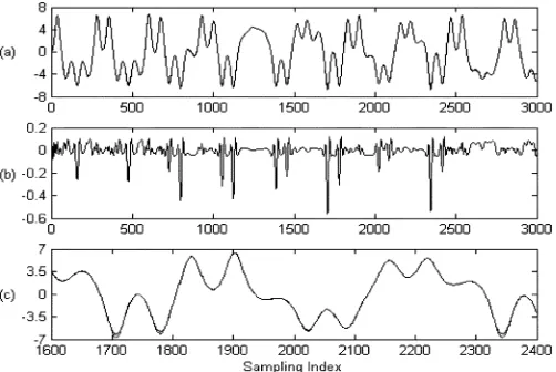
[image:9.594.302.553.65.233.2]. The recovered system output from the model (30) was compared with that from the original model (28) over the validation set and is shown in Fig. 2(a) and (b), which clearly indicates that the model (30) provides an excellent representation for the input–output data set generated from the system (28) with an input of sine wave. For a closer inspection of the result, the interval [1600, 2400], where the maximum errors appear as shown in (b), was expanded and this is shown in Fig. 2(c). Note that model predicted outputs or
Fig. 2. Comparison of the model output based on the WN (30) with the measurements over the test set. (a) Overlap of the output of the WN (30) and the measurements. (b) Discrepancy between the output of the WN (30) and the measurements. (c) The interval[1600; 2400] was expanded for a closer inspection. In (a) and (c), the solid lines indicate the measurements and the dashed lines indicate the model predicted outputs.
the long term model predictions are used here as a much more severe test compared with one-step-ahead predicted outputs. For comparison, we have also tried other wavelet models using only the total-variable-involved functional exponent in (29) by expanding this exponent using a 3-D radial wavelet decomposition (a traditional 3-D fixed grid WN). For example, with the same input–output data set and the same wavelet parameters as did in the model (29), the 3-D Mexican hat radial wavelet was used to fit a model. It was calculated that the root-mean-square-error (RMSE) of the model prediction over the test data set (points from 1001 to 3000) is 0.0889 for the traditional wavelet model. The value of RMSE with respect to the same test data set based on the proposed method, however, is only 0.0213, which is much smaller. This implies that for this example the new proposed WN may be advantageous over a conventional fixed grid WN, where only the total-variable-involved functional exponent were considered.
B. High-Dimensional Chaotic System
Consider the Mackey–Glass delay-differential equation [57]
(31)
where the time delay was chosen to be 30 in this example. This example was chosen to facilitate comparisons with other results [25], [58]. Setting the initial condition 0.9 for , a Runge–Kutta integral algorithm was applied to calculate (31) with an integral step 0.01 and 6000
equi-spaced samples, , were recorded with
a sampling interval of 0.06 time units.
tests. Following [59], the dimension of the recorded time series was assumed to be 6, and the significant variables were
therefore chosen to be .
Sim-ilar to the previous example, the initial WN was chosen to be
(32)
where the 1-D, 2-D, and 3-D compactly supported Mexican hat radial WNs were used in this example to approximate the univar-iale functions , the bivariate functions , and the tri-variate function , respectively, with the coarsest resolutions
and finest resolutions , and . A forward OLS-ERR algorithm was used to select significant model terms. The final identified model was found to be
(33)
where and
are the 1-D and 2-D compactly supported Mexican hat wavelets, .
Most of the results in the literature concern one-step-ahead predictions of the sampled time series. In this example, however, two-step-ahead predictions were considered and the predicted results were compared with previous studies [25], [58], where only one-step-ahead predictions were considered. To facilitate comparisons, a measurement index, the relative error [25], was used to measure the performance of the identified WN. This index is defined as
(34)
[image:10.594.301.552.64.247.2] [image:10.594.43.286.122.219.2]where and are the measurements on the test set and asso-ciated two-step-ahead predictions, respectively.
Fig. 3. Two-step-ahead predictions for the Mackey–Glass delay-differential (31) using the identified WN (33) over the validation set. The stars “3” indicate the measurements and the circles “” indicate the predications. To allow a clear inspection, the data are plotted once every 100 points.
Fig. 4. Relative errors between the two-step-ahead predictions from the identified WN (33) and the measurements for the Mackey–Glass delay-differential (31) over the validation set.
[image:10.594.303.551.309.480.2]Fig. 5. Sunspot time series for the period from 1700 to 1999.
C. The Sunspot Time Series
The sunspot time series considered in this example consists of 300 annually recorded Wolf sunspots of the period from 1700 to 1999, see Fig. 5. The objective here is to identify a WN model to produce one-step-ahead predictions for the sunspot data set. Again, the original measurements were initially normalized into the unit interval using the infor-mation . Designate the normalized sequence by . The data set was separated into two parts: the training set consisted of 250 data points corresponding to the period 1700–1949, and the test set consisted of 50 data points corre-sponding to the period 1950–1999.
Following [56], the model order was chosen to be 9 here, and the most significantvariables were chosen to be ,
and . The initial WN model was therefore chosen to be
(35)
where for ,
for 1,2, and . The 1-D, 2-D, and 3-D
compactly supported Gaussian radial WNs were used in this ex-ample to approximate the univariate functions , the bivariate functions , and the tri-variate function , respectively, with the coarsest resolutions and finest res-olutions . A forward OLS-ERR algorithm [35], [36] was used to select significant model terms. The final identified model was found to be
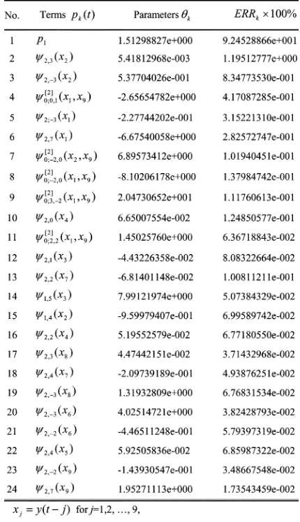
(36)
where are the wavelet terms formed by compactly sup-ported Gaussian wavelets. The identified wavelet terms, the corresponding parameters, and the associated ERRs are listed in Table I. Roughly speaking, the values of the ERRs provide an index indicting the contribution made by the corresponding model term to a signal of interest, and in general, the larger a ERR value is, the more significant the corresponding model term is for representing a given signal. For details about the meaning of ERR, see [25] and [36]. The result of the
TABLE I
WAVELETTERMS, PARAMETERS,ANDASSOCIATEDERRORREDUCTION
RATIOS FOR THESUNSPOTTIMESERIES
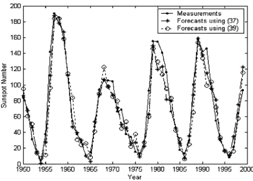
one-step-ahead predictions based on the WN (36) over the test set is shown in Fig. 6 (the dashed-star line), which clearly shows that the identified model provides an excellent representation for the sunspot time series.
In order to compare the predicted result of the WN with other work [60], the following index, the mean-square-error on the test set, was used to measure the performance of the identified WN
(37)
pre-Fig. 6. One-step-ahead predictions for the sunspot time series based the WNs (36) and (38) over the test set. The point-solid line indicates the measurements, the dashed-star line indicates the predictions from (36), and the dotted-circle line indicates the predications from (38).
dictions, respectively, and . It was cal-culated 0.0651 for the identified WN (36) that is smaller than 0.076 (for the period of years 1921–1954) and 0.23 (for the period of years 1955–1979) which are given by a wavelet decomposition model proposed in [60].
An important point revealed by Table I is that the three
vari-ables , and are far more significant
than the other variables. This is consistent with the result given in [55]. In fact, the sunspot time series can be satisfactory de-scribed using a WN with respect to only these three significant variables. This model is given in the following:
(38)
The one-step-ahead predictions from the WN (38) over the test set is shown in Fig. 6 (the dotted-circle line), where the normalized error was calculated to be 0.1044, which is still very small.
VI. CONCLUSION
A new class of WNs has been introduced for nonlinear system identification. The main advantage of the new identification ap-proach compared with existing WNs, is that the new WNs are more practical and can be applied to problems in medium and high dimensions. This property arises due to the fact that the structure of the new WNs are based on ANOVA expansions, for
which the high-dimensional subfunctions (submodels) can often be neglected for many nonlinear systems.
It has been noted that a conventional WN always includes the total-variables-involved wavelet terms, even though this is not necessary for most systems in the real world. In addition, a model that includes only high-order terms is liable to produce a deleterious effect on the output behavior of the model which can induce spurious dynamics. The new WNs avoid most of these problems by decomposing a multidimensional function into a number of low-dimensional submodels.
In theory, many types of wavelets can be used to approximate the low-dimensional submodels by a scheme of taking tensor products or adopting radial functions. In network training, how-ever, it is often preferable to use a wavelet that is compactly sup-ported, since the number of compactly supported wavelets at a given resolution scale can be determined beforehand and, thus, the total number of candidate wavelet terms involved in the net-work becomes known. Radial wavelets are not compactly sup-ported but rapidly vanishing. It is therefore reasonable to trun-cate a radial wavelet to make it quasi-supported, this can then be used as a normal compactly supported wavelet to implement a WN. Most radial wavelets including the Gaussian and Mexican hat wavelets are easy to calculate with a very small computa-tional load and can therefore be chosen to implement the WN. Other nonradial wavelets, which are either compactly supported or not, can also be used if there is strong evidence that these wavelets can easily be used to implement a WN.
A WN may involve a great number of wavelet terms for a high-dimensional system. However, in most cases many of the model terms are redundant and only a small number of signif-icant terms are necessary to describe a given nonlinear system with a given accuracy. In the present study, an efficient term de-tection algorithm was employed to train the new WNs to yield parsimonious models.
In summary, the new WNs appear to be advantageous com-pared to conventional wavelet modeling schemes and provide an effective approach for nonlinear system identification. The results obtained from the bench test examples demonstrate the effectiveness of the new identification procedure.
APPENDIX
FORWARDOLS ALGORITHM AND THEERR
The OLS algorithm [35], [36] was initially introduced to select the most significant model terms and estimate the model parameters simultaneously for all linear-in-the-parameter models. Consider the linear-in-the-parameters model (21),
where the regression matrix with,
, is the length of the obser-vational data set. With the assumption that is full rank in columns, then can be orthogonally decomposed as
(39)
where is an unit upper triangular matrix and is an matrix with orthogonal columns
in the sense that with
. Model (21) can then be expressed as
[image:12.594.40.288.63.241.2]where are the observations of the system output, is the parameter vector, is the vector of the noise signal, and is an auxiliary parameter vector, which can be calculated directly from and by means of the property of orthogonality as
(41)
The parameter vector , which is related to by the equation , can easily be calculated by solving this equation using a substitution scheme.
The number of all the candidate terms in model (21) is often very large. Some of these terms may be redundant and should be removed to give a parsimonious model with only terms . Detection of the significant model terms can be achieved using the OLS procedures described in the fol-lowing.
Assume that the residual signal in the model (21) is un-correlated with the past outputs of the system, then the output variance can be expressed as
(42)
Note that the output variance consists of two parts, the desired output which can be explained by the re-gressors, and the part which represents the unex-plained variance. Thus, is the increment to the explained desired output variance brought by , and the
th ERR , introduced by , can be defined as
ERR
(43)
This ratio provides a simple but effective means for seeking a subset of significant regressors. The significant terms can be selected in a forward-regression manner according to the value of ERR step by step. The selection procedure can be terminated
at the th step when ERR , where
is a desired error tolerance, or cutoff value, which can be learnt during the regression procedure. The final model is the linear combination of the significant terms selected from the candidate terms
(44)
which is equivalent to
(45)
where the parameters can be calculated in the selection procedure. Note that, since most significant model terms can be selected in a forward-regression manner step by
step, or a term at a time, the assumption that the regression ma-trix is full rank in columns becomes unnecessary [56].
REFERENCES
[1] C. K. Chui,An Introduction to Wavelets. New York: Academic, 1992. [2] I. Daubechies, Ten Lectures on Wavelets. Philaelphia, PA: SIAM,
1992.
[3] Y. Meyer,Wavelets: Algorithms and Applications. Philaelphia, PA: SIAM, 1993.
[4] S. Chen, S. A. Billings, and P. M. Grant, “Nonlinear system identifica-tion using neural networks,”Int. J. Control, vol. 51, pp. 1191–1214, Jun. 1990.
[5] S. Chen and S. A. Billings, “Neural networks for nonlinear system mod-eling and identification,”Int. J. Control, vol. 56, pp. 319–346, Aug. 1992.
[6] S. Chen, S. A. Billings, and P. M. Grant, “Recursive hybrid algorithm for nonlinear system identification using radial basis function networks,” Int. J. Control, vol. 55, pp. 1051–1070, May 1992.
[7] K. S. Narendra and K. Parthasarathy, “Identification and control of dy-namical systems using neural networks,”IEEE Trans. Neural Netw., vol. 2, no. 2, pp. 252–262, Mar. 1991.
[8] S. A. Billings, H. B. Jamaluddin, and S. Chen, “Properties of neural networks with applications to modeling nonlinear dynamic systems,” Int. J. Control, vol. 55, pp. 193–224, Jan. 1992.
[9] S. A. Billings and S. Chen, “The determination of multivariable nonlinear models for dynamic systems using neural networks,” in Neural Network Systems Techniques and Applications, C. T. Leondes, Ed. New York: Academic, 1998, pp. 231–278.
[10] P. S. Sastry, G. Santharam, and K. P. Unnikrishnan, “Memory neuron networks for identification and control of dynamical systems,”IEEE Trans. Neural Netw., vol. 5, no. 3, pp. 306–319, May 1994.
[11] S. Haykin, Neural Networks: A Comprehensive Foundation. New York: Macmillan, 1994.
[12] T. N. Lin, B. G. Horne, P. Tino, and C. L. Giles, “Learning long-term dependencies in NARX recurrent neural networks,”IEEE Trans. Neural Netw., vol. 7, no. 6, pp. 1329–1338, Nov. 1996.
[13] K. S. Narendra and S. Mukhopadhyay, “Adaptive control using neural networks and approximate models,”IEEE Trans. Neural Netw., vol. 8, no. 3, pp. 475–485, May 1997.
[14] N. B. Karayiannis and M. M. Randolph, “On the construction and training of reformulated radial basis function networks,”IEEE Trans. Neural Netw., vol. 14, no. 4, pp. 835–846, Jul. 2003.
[15] I. Rivals and L. Personnaz, “Neural-network construction and selection in nonlinear modeling,”IEEE Trans. Neural Netw., vol. 14, no. 4, pp. 804–819, Jul. 2003.
[16] R. J. Wai and H. H. Chang, “Backstepping wavelet neural network control for indirect field-oriented induction motor drive,”IEEE Trans. Neural Netw., vol. 15, no. 2, pp. 367–382, Mar. 2004.
[17] H. H. Szu, B. Telfer, and S. Kadambe, “Neural network adaptive wavelets for signal representation and classification,”Opt. Eng., vol. 31, pp. 1907–1916, Sep. 1992.
[18] Q. H. Zhang and A. Benveniste, “Wavelet networks,” IEEE Trans. Neural Netw., vol. 3, no. 6, pp. 889–898, Nov. 1992.
[19] Y. C. Pati and P. S. Krishnaprasad, “Analysis and synthesis of feedfor-ward neural networks using discrete affine wavelet transforms,”IEEE Trans. Neural Netw., vol. 4, no. 1, pp. 73–85, Jan. 1993.
[20] J. G. Daugman, “Complete discrete 2-D gabor transforms by neural networks for image analysis and compression,”IEEE Trans. Acoust., Speech, Signal Process., vol. 36, no. 7, pp. 1169–1179, Jul. 1988. [21] H. Dickhaus and H. Heinrich, “Classfying biosignals with wavlet
net-works,”IEEE Eng. Med. Biol. Mag., vol. 15, no. 5, pp. 103–111, Sep. 1996.
[22] S. Pittner, S. V. Kamarthi, and Q. G. Gao, “Wavelet networks for sensor signal classification in flank wear assessment,”J. Intell. Manufact., vol. 9, pp. 315–322, Aug. 1990.
[23] K. W. Wong and A. C.-S. Leung, “On-line successive synthesis of wavelet networks,”Neural Process. Lett., vol. 7, pp. 91–100, Apr. 1998. [24] E. A. Rying, G. L. Bilbro, and J. C. Lu, “Focused local learning with wavelet neural networks,”IEEE Trans. Neural Netw., vol. 13, no. 2, pp. 304–319, Mar. 2002.
[25] L. Y. Cao, Y. G. Hong, H. P. Fang, and G. W. He, “Predicting chaotic time series with wavelet networks,”Phys. D, vol. 85, pp. 225–238, Jul. 1995.
[27] Y. Oussar and G. Dreyfus, “Initialization by selection for wavelet net-work training,”Neurocomput., vol. 34, pp. 131–143, Sep. 2000. [28] J. H. Friedman, “Multivariate adaptive regression splines,”Ann. Statist.,
vol. 19, pp. 1–67, Mar. 1991.
[29] Z. H. Chen, “Fitting multivariate regression functions by interaction spline models,”J. Roy. Stat. Soc. B Met., vol. 55, pp. 473–491, 1993. [30] J. Zhang, G. G. Walter, Y. Miao, and W. N. W. Lee, “Wavelet neural
networks for function learning,”IEEE Trans. Signal Process., vol. 43, no. 6, pp. 1485–1497, Jun. 1995.
[31] Q. H. Zhang, “Using wavelet network in nonparametric estimation,” IEEE Trans. Neural Netw., vol. 8, no. 2, pp. 227–236, Mar. 1997. [32] S. Ferrari, M. Maggioni, and N. A. Borghese, “Multoresolution
approx-imation with hierarchical radial basis functions networks,”IEEE Trans. Neural Netw., vol. 15, no. 1, pp. 178–188, Jan. 2004.
[33] D. Coca and S. A. Billings, “Continuous-time system identification for linear and nonlinear system identification using wavelet decomposi-tions,”Int. J. Bifurcat. Chaos, vol. 7, pp. 87–96, Jan. 1997.
[34] S. A. Billings and D. Coca, “Discrete wavelet models for identification and qualitative analysis of chaotic systems,”Int. J. Bifurcat. Chaos, vol. 9, pp. 1263–1284, Jul. 1999.
[35] S. A. Billings, S. Chen, and M. J. Korenberg, “Identification of MIMO nonlinear systems suing a forward regression orthogonal estimator,”Int. J. Control, vol. 49, pp. 2157–2189, Jun. 1989.
[36] S. Chen, S. A. Billings, and W. Luo, “Orthogonal least squares methods and their application to nonlinear system identification,”Int. J. Control, vol. 50, pp. 1873–1896, Nov. 1989.
[37] S. Chen, C. F. N. Cowan, and P. M. Grant, “Orthogonal least-squares learning algorithm for radial basis function networks,” IEEE Trans. Neural Netw., vol. 2, no. 2, pp. 302–309, Mar. 1991.
[38] I. J. Leontaritis and S. A. Billings, “Input-output parametric models for nonlinear systems-part I: Deterministic nonlinear systems; part II: Sto-chastic nonlinear systems,”Int. J. Control, vol. 41, pp. 303–344, 1985. [39] R. K. Pearson, “Nonlinear input/output modeling,”J. Process Contr.,
vol. 5, pp. 197–211, Aug. 1995.
[40] , “Nonlinear process identification,” inNonlinear Process Control, M. A. Henson and D. E. Seborg, Eds. Englewood Cliffs, NJ: Prentice-Hall, 1997, pp. 11–110.
[41] L. A. Aguirre, “Application of global models in the identification, anal-ysis and control of nonlinear dynamics and chaos,” Ph.D. dissertation, Dept. Autom. Control Syst. Eng., Univ. Sheffield, Sheffield, U.K., 1994. [42] N. Chiras, “Linear and nonlinear modeling of gas turbine engines,” Ph.D. dissertation, School Electron., Univ. Glamorgan, Wales, U.K., 2002.
[43] R. K. Pearson,Discrete-Time Dynamic Models. Oxford, U.K.: Oxford Univ. Press, 1999.
[44] G. Y. Li, C. Rosenthal, and H. Rabits, “High dimensional model repre-sentations,”J. Phys. Chem. A, vol. 105, pp. 7765–7777, Aug. 2001. [45] H. L. Wei and S. A. Billings, “A unified wavelet-based modeling
frame-work for nonlinear system identification: The WANARX model struc-ture,”Int. J. Control, vol. 77, pp. 351–366, Mar. 2004.
[46] J. Gonzalez, I. Rojas, J. Ortega, H. Pomares, F. J. Fernandez, and A. F. Diaz, “Multiobjective evolutionary optimization of the size, shape, and position parameters of radial basis functions networks for function ap-proximation,”IEEE Trans. Neural Netw., vol. 14, no. 6, pp. 1478–1495, Nov. 2003.
[47] S. G. Mallat, “A theory for multiresolution signal decomposition: The wavelet representation,”IEEE Trans. Pattern Anal. Mach. Intell., vol. 11, pp. 674–693, Jul. 1989.
[48] ,A Wavelet Tour of Signal Processing. New York: Academic, 1998.
[49] L. X. Wang and J. M. Mendel, “Fuzzy basis functions, universal approx-imations, and orthogonal least squares learning,”IEEE Trans. Neural Netw., vol. 3, no. 5, pp. 807–814, Sep. 1992.
[50] X. Hong and C. J. Harris, “Nonlinear model structure detection using op-timum experimental design and orthogonal least squares,”IEEE Trans. Neural Netw., vol. 12, no. 2, pp. 435–439, Mar. 2001.
[51] X. Hong, P. M. Sharkey, and K. Warwick, “A robust nonlinear identi-fication algorithm using PRESS statistic and forward regression,”IEEE Trans. Neural Netw., vol. 14, no. 2, pp. 454–458, Mar. 2003.
[52] S. A. Billings and H. L. Wei, “The wavelet-NARMAX representation: A hybrid model structure combining polynomial models with multires-olution wavelet decompositions,” Int. J. Syst. Sci., to be published. [53] S. A. Billings and W. S. F. Voon, “Correlation based model validity tests
for nonlinear models,”Int. J. Control, vol. 44, pp. 235–244, Jul. 1986. [54] S. A. Billings and Q. M. Zhu, “Nonlinear model validation using
corre-lation tests,”Int. J. Control, vol. 60, pp. 1107–1120, Dec. 1994. [55] D. Coca, “A class of wavelet multiresolution decompositions for
non-linear system identification and signal processing,” Ph.D., Dept. Autom. Control Syst. Eng., Univ. Sheffield, Sheffield, U.K., 1996.
[56] H. L. Wei, S. A. Billings, and J. Liu, “Term and variable selection for nonlinear system identification,”Int. J. Control, vol. 77, pp. 86–110, Jan. 2004.
[57] M. C. Mackey and L. Glass, “Oscillation and chaos in physiological control systems,”Science, vol. 197, pp. 287–289, Jul. 1977.
[58] R. Bone, M. Crucianu, and J.-P. A. de Beauville, “Learning long-term dependences by the selective additional time-delayed connetions to recurrent neural networks,”Neurocomput., vol. 48, pp. 251–266, Oct. 2002.
[59] M. Casdagli, “Nonlinear prediction of chaotic time series,”Phys. D, vol. 35, pp. 335–356, May 1989.
[60] S. Soltani, “On the use of wavelet decomposition for time series predic-tion,”Neurocomput., vol. 48, pp. 267–277, Oct. 2002.
Stephen A. Billingsreceived the B.Eng. degree in electrical engineering (first class honors) from the University of Liverpool, Liverpool, U.K., in 1972, the Ph.D. degree in control systems engineering from the University of Sheffield, Sheffield, U.K., in 1976, and the D.Eng. degree from the University of Liverpool in 1990.
He was appointed as Professor in the Department of Automatic Control and Systems Engineering, Uni-versity of Sheffield, in 1990 and leads the Signal Pro-cessing and Complex Systems research group. His research interests include system identification and information processing for nonlinear systems, narmax methods, model validation, prediction, spectral anal-ysis, adaptive systems, nonlinear systems analysis and design, neural networks, wavelets, fractals, machine vision, cellular automata, spatio–temporal systems, fMRI and optical imagery of the brain, metabolic systems engineering, systems biology, and related fields.
Dr. Billings is a Chartered Engineer (C.Eng.), Chartered Mathematician (C.Math.), a Fellow of the Institution of Electrical Engineers (IEEE-U.K.) and a Fellow of the Institute of Mathematics and Its Applications.
Hua-Liang Weireceived the B.Sc. degree in math-ematics from Liaocheng University, Liaocheng, China, in 1989, the M.Sc. degree in automatic control from the Beijing Institute of Technology, Beijing, China, in 1992, and the Ph.D. degree in signal processing and control engineering from the University of Sheffield, Sheffield, U.K., in 2004.