Few-cycle optical rogue waves: Complex modified Korteweg-de Vries equation

This is a repository copy of Few-cycle optical rogue waves: Complex modified Korteweg-de Vries equation.

White Rose Research Online URL for this paper: http://eprints.whiterose.ac.uk/106790/

Version: Accepted Version

Article:

He, J., Wang, L., Li, L. et al. (2 more authors) (2014) Few-cycle optical rogue waves: Complex modified Korteweg-de Vries equation. Physical Review E, 89 (6). 062917. ISSN 2470-0045

https://doi.org/10.1103/PhysRevE.89.062917

[email protected] https://eprints.whiterose.ac.uk/

Reuse

Unless indicated otherwise, fulltext items are protected by copyright with all rights reserved. The copyright exception in section 29 of the Copyright, Designs and Patents Act 1988 allows the making of a single copy solely for the purpose of non-commercial research or private study within the limits of fair dealing. The publisher or other rights-holder may allow further reproduction and re-use of this version - refer to the White Rose Research Online record for this item. Where records identify the publisher as the copyright holder, users can verify any specific terms of use on the publisher’s website.

Takedown

If you consider content in White Rose Research Online to be in breach of UK law, please notify us by

FEW-CYCLE OPTICAL ROGUE WAVES: COMPLEX MODIFIED KORTEWEG-DE VRIES EQUATION

JINGSONG HE†∗_{, LIHONG WANG†, LINJING LI†, K.PORSEZIAN‡AND R. ERD´ELYI§}

†Department of Mathematics, Ningbo University, Ningbo, Zhejiang 315211, P. R. China

‡Department of Physics, Pondicherry University, Pondicherry-605014, India

§Solar Physics and Space Plasma Research Centre, University of Sheffield, Sheffield, S3 7RH, UK

Abstract. _{In this paper, we consider the complex modified Korteweg-de Vries (mKdV)}

equa-tion as a model of few-cycle optical pulses. Using the Lax pair, we construct a generalized Darboux transformation and systematically generate the first-, second- and third-order rogue wave solutions and analyze the nature of evolution of higher-order rogue waves in detail. Based on detailed numerical and analytical investigations, we classify the higher-order rogue waves with respect to their intrinsic structure, namely, fundamental pattern, triangular pattern, and ring pattern. We also present several new patterns of the rogue wave according to the standard and non-standard decomposition. The results of this paper explain the generalization of higher-order rogue waves in terms of rational solutions. We apply the contour line method to obtain the analytical formulas of the length and width of the first-order RW of the complex mKdV and the NLS equations. In nonlinear optics, the higher-order rogue wave solutions found here will be very useful to generate high-power few-cycle optical pulses which will be applicable in the area of ultra-short pulse technology.

Keywords: complex MKdV equation, Darboux transformation, rogue wave.

PACS number(s): 05.45.Yv, 42.65.Tg, 03.75.Lm, 87.14.gk

1. Introduction

The theory of nonlinear dynamics has attracted considerable interest and is fundamentally linked to several basic developments in the area of soliton theory. It is well-known that the Korteweg-de Vries (KdV) equation, modified Korteweg-de Vries (mKdV) equation, sine Gordon equation and the nonlinear Schr¨odinger (NLS) equation are the most typical and well-studied integrable evolution equations which describe nonlinear wave phenomena for a range of disper-sive physical systems. Their stable multi-soliton solutions play an important role in the study of nonlinear waves [1]. Further studies have also been carried out to examine the effects on these solitons due to dissipation, inhomogeneity or non-uniformity present in nonlinear media [2, 3].

The term “soliton” is a sophisticated mathematical concept that derives its name from the word “solitary wave” which is a localized wave of translation that arises from the balance between nonlinear and dispersive effects [1]. In spite of the initial theoretical investigations, the concept of solitary wave could not gain wide recognition for a number of years in the midst of excitement created by the development of electromagnetic concepts in those times. Korteweg and de Vries (1895) developed a mathematical model for the shallow water problem and demonstrated the possibility of solitary wave generation [4]. Next, the study of solitary waves really took off in the mid-1960s when Zabusky and Kruskal discovered the remarkably stable particle-like behaviour of solitary waves [5]. They reported numerical experiments where

∗_{Corresponding Author: Email: [email protected], Tel: 86-574-87600739, Fax: 86-574-87600744.} 1

solitary waves, described by the KdV equation, passed through each other unchanged in speed or shape, which led them to coin the word “soliton” to suggest such a unique property. In a follow-up study Zakharov and Shabat generalized the inverse scattering method in 1972 and also solved the nonlinear Schr¨odinger equation, demonstrating both its integrability and the existence of soliton solutions [6].

Following the above discoveries, solitary waves of all flavors advanced rapidly in many areas of science and technology. In nonlinear physics applications to many areas e.g. hydrodynamics, biophysics, atomic physics, nonlinear optics, etc., have been developed. As of now, more than a few hundreds of nonlinear evolution equations (NEEs) have been shown to admit solitons and some of these theoretical equations are also responsible for the experimental discovery of solitons [1,7]. In general, nonlinear phenomena are often modelled by nonlinear evolution equa-tions exhibiting a wide range of high complexities in terms of difference in linear and nonlinear effects. In the past four decades or so, the advent of high-speed computers, many advanced mathematical softwares and the development of a number of sophisticated and systematic ana-lytical methods, which are well-supported by experiments have encouraged both theoreticians and experimentalists. Nonlinear science has experienced an explosive growth by the invention of several exciting and fascinating new concepts not just like solitons, but e.g. dispersion-managed solitons, rogue waves, similaritons, supercontinuum generation, etc. [1]. Many of the completely integrable nonlinear partial differential equations (NPDEs) admit one of the most striking aspects of nonlinear phenomena, which describe soliton as a universal character and they are of great mathematical as well as physical interest. It is impossible to discuss all these manifestations exhaustively in this paper. We further restrict ourselves to the solitary wave manifestation in nonlinear optics. In the area of soliton research at the forefront, right now, is the study of optical solitons, where the highly sought-after goal is to use strong localized nonlinear optical pulses as the high-speed information-carrying bits in optical fibers.

Optical solitons are localized electromagnetic waves that propagate steadily in a nonlinear medium resulting from the robust balance between nonlinearity and linear broadening due to dispersion and diffraction. Existence of the optical soliton was first time found in 1973 when Hasegawa and Tappert demonstrated the propagation of a pulse through a nonlinear optical fiber described by the nonlinear Schr¨odinger equation [8]. They performed a number of com-puter simulations demonstrating that nonlinear pulse transmission in optical fibers would be stable. Subsequently, after the fabrication of low-loss fiber, Mollenauer et al. in 1980 success-fully confirmed this theoretical prediction of soliton propagation in a laboratory experiment [7]. Since then, fiber solitons have emerged as a very promising potential candidate in long-haul fiber optic communication systems.

Further, in addition to several important developments in soliton theory, the concept of modulational instability (MI) has also been widely used in many nonlinear systems to explain why experiments involving white coherent light supercontinuum generation (SCG), admit a triangular spectrum which can be described by the analytical expressions for the spectra of Akhmediev breather solutions at the point of extreme compression [1]. In the case of the NLS equation, Peregrine already in [9] had identified the role of MI in the formation of patterns resembling high-amplitude freak waves or rogue wave (RW). RWs have recently been also reported in different areas of science. In particular, in photonic crystal fibre RWs are well-established in connection with SCG [10]. This actually has stimulated research for RWs in other physical systems and has paved the way for a number important applications, including the control of RWs by means of SCG [11, 12], as well as studies in e.g. superfluid Helium [13], Bose Einstein condensates [14], plasmas [15, 16], microwave [17], capillary phenomena [18],

telecommunication data streams [19], inhomogeneous media [20], water experiments [21], and so on. Recently, Kibler et al. _{[22] using a suitable experiment with optical fibres were able}

to generate femtosecond pulses with strong temporal and spatial localization and near-ideal temporal Peregrine soliton characteristics.

For the past couple of years, several nonlinear evolution equations were shown to exhibit the RW-type rational solutions [23–39]. From the above listed works, it is clear that one of the possible generating mechanisms [40] for the higher-order RW is the interaction of multiple breathers possessing identical and very particular frequency of the underlying equation. Though the theory of solitons and many mathematical methods have been well-used in connection with soliton theory for the past four decades or so, to the best of our knowledge, the dynamics of multi-rogue wave evolutions has not yet been systematically investigated in integrable nonlinear systems [41].

Very recently, considering the propagation of few-cycle optical pulses in cubic nonlinear media and by developing multiple scaling approach to the Maxwell-Bloch-Heisenberg equation up to the third-order in terms of expansion parameter, the complex mKdV equation was derived [42, 43]. Circularly polarized few-cycle optical solitons were found which are valid for long pulses. Thus, it is more than worthy to systematically investigate the existence of the few-cycle optical rogue waves for this model, and this is the main purpose of the present paper.

The organization of this paper is as follows. In Section 2, based on the parameterized Darboux transformation (DT) of the mKdV equation, the general formation of the solution is given. In Section 3, we construct the higher-order rogue waves from a periodic seed with constant amplitude and analyze their structures in detail by choosing suitable system parameters. We provide detailed discussion about the obtained results in Sections 4 and 5.

2. The Darboux Transformation

For our analysis, we begin with coupled complex mKdV equations of the form of

qt+qxxx−6qrqx = 0, (1)

rt+rxxx−6rqrx = 0. (2)

Under a reduction condition q = ₋r∗_{, the above coupled equations reduce to the complex}

mKdV

qt+qxxx+ 6|q|2qx = 0. (3) The complex mKdV equation is one of the well-known and completely integrable equations in soliton theory, which possesses all the basic characters of integrable models. From a physical point of view, the above equation has been derived for, e.g. the dynamical evolution of non-linear lattices, plasma physics, fluid dynamics, ultra-short pulses in nonnon-linear optics, nonnon-linear transmission lines and so on [41]. The Lax pair corresponding to the coupled mKdV equations is given by [41], i.e.

ψx =M ψ, (4)

ψt= (V3λ3+V2λ2+V1λ+V0)ψ =N ψ, (5)

with ψ = φ1 φ2

, M =

−iλ q r iλ

, V3 =

−4i 0 0 4i

,

V2 =

0 4q

4γ 0

, V1 =

−2iqr 2iqx −2irx 2iqr

,

V0 =

−qrx+qxr −qxx+ 2q2r −rxx+ 2qr2 qrx−qxr

.

Here, λ is an arbitrary complex spectral parameter or also called eigenvalue, and ψ is the eigenfunction corresponding to λ of the complex mKdV equation. From the compatibility condition Mt− Nx + [M, N] = 0, one can easily obtain the coupled equations (1) and (2). Furthermore, set T be a gauge transformation by

ψ[1] =T ψ, q _→q[1], r_→r[1], (6) and

ψ[1]

x =M[1]ψ[1], M[1] = (Tx+T M)T−1, (7)

ψ[1]t =N[1]ψ[1], N[1] = (Tt+T N)T−1. (8) Here, M[1] _{=M(→ q}[1]_{, r →r}[1]_{), N}[1] _{=N(q →q}[1]_{, r →r}[1]_{). By cross-differentiating (7) and}

(8), we obtain

Mt[1] −Nx[1] + [M

[1]_{, N}[1]_{] =T(M}

t−Nx+ [M, N])T−1. (9)

This implies that, in order to prove that the mKdV equation is invariant under the gauge transformation (6), it is important to look for determine the T such that M[1]_{, N}[1] _{have the}

same forms as M, N. Meanwhile, the seed solutions (q, r) in spectral matrixes M, N are mapped into the new solutions (q[1]_{, r}[1]_{) in terms of transformed spectral matrixesM}[1]_{, N}[1]_.

Recently, using the generalized Darboux transformation,nth-order rogue wave solutions for the complex mKdV equation have been proposed in e.g. [38]. However, in our work, we shall systematically analyze the evolution of the different patterns of higher-order rogue waves by suitably choosing the parameters in the rational solutions. In addition, it is worth to note that the obtained results are in agreement with our recently published developments about the method of generating higher-order rogue waves [39, 40].

2.1 One-fold Darboux Transformation

From the knowledge of the known form of the DT for the nonlinear Schr¨odinger equation [44–49], we assume that a trial Darboux matrix T in eq. (6) has the following form

T =T(λ) =

a1 b1 c1 d1

λ+

a0 b0 c0 d0

, (10)

wherea0, b0, c0, d0, a1, b1,c1, d1 are functions of x and t. From

Tx+T M =M[1]T, (11)

by comparing the coefficients of λj_{, j = 2,1,0, it yields}

λ2 :b1 = 0, c1 = 0,

λ1 :a1x = 0, −2ib0+q1d1−qa1 = 0, d1x = 0, −rd1 +r1a1 + 2ic0 = 0, λ0 _:q

1c0−a0x−rb0 = 0, −b0x+q1d0−qa0 = 0,

r1a0−c0x−rd0 = 0, r1b0−d0x−qc0 = 0. (12)

From the coefficients of λ1_{, we conclude that a}

1 and d1 are functions of t only. Similarly, from

Tt+T N =N[1]T, (13)

and by comparing the coefficients ofλj_{, j = 3,2,1,0, we obtain the following set of equations}

λ3 :q1d1−qa1−2ib0 = 0, r1a1−rd1+ 2ic0 = 0,

λ2 :₋q1r1a1i+ 2q1c0+a1qri−2rb0 = 0, −a1qxi+ 2q1d0−2qa0+q1xd1i= 0,

2r1a0−r1xa1i−2rd0+d1rxi= 0, q1r1d1i+ 2r1b0−2qc0−d1qri= 0,

λ1 :₋a1t+r1q1xa1+a1qrx−a1rqx+ 2iq1xc+ 2ib0rx−2iq1r1a0+ 2ia0qr−q1r1xa1 = 0,

−2iq1r1b0−2ib0qr+a1qxx+ 2iq1xd0−2ia0qx−2a1q2r−q1xxd1+ 2q12r1d1 = 0,

−r1xxa1+ 2iq1r1c0+ 2q1r12a1+ 2iqrc0−2ia0r1x+ 2id0rx−2d1qr2 +d1rxx = 0, −d1t−2ic0qx+ 2iq1r1d0−r1q1xd1−2ir1xb0−d1qrx+d1rqx−2id0qr+q1r1xd1 = 0, λ0 :₋q1xxc0+b0rxx+ 2q21r1c0+a0qrx−2b0qr2 +r1q1xa0 −q1r1xa0−a0rqx−a0t= 0,

a0qxx−b0qrx−b0q1r1x−2a0q2r+r1q1xb0+ 2q12r1d0+b0rqx−q1xxd0−b0t= 0, −r1xxa0+d0rxx−r1q1xc0+ 2q1r21a0+q1r1xc0−c0rqx+c0qrx−2d0qr2−c0t= 0, −r1q1xd0+q1r1xd0−r1xxb0+ 2q1r21b0+c0qxx+d0rqx−d0qrx−2c0q2r−d0t= 0.(14) By making use of eq. (12) and eq. (14), one may obtain a1x = 0, d1x = 0, a1t = 0, d1t = 0, which implies that a1 and d1 are two constants.

In order to obtain the non-trivial solutions of the complex mKdV equation, we provide the Darboux transformation under the condition a1 = 1, d1 = 1. Without loss of generality, and

based on eqs. (12) and (14), we observe that the Darboux matrix T admits the following form

T =T(λ) =

1 0 0 1 λ+

a0 b0 c0 d0

. (15)

Here, a0, b0, c0, d0 are functions of x and t, which could be expressed by two eigenfunctions

corresponding toλ1 andλ2. To begin with, we introduce 2neigenfunctionsψj and 2nassociated distinct eigenvalues λj as follows

ψj =

φj1 φj2

, j = 1,2, ...2n, φj1 =φ1(x, t, λj), φj2 =φ2(x, t, λj). (16)

Noteφ1(x, t, λ) andφ2(x, t, λ) are two components of eigenfunctionψ associated with λ in eqs.

(4) and (5). Here, it is worthwhile to note that since the eigenfunction

ψj =

φj1 φj2

is the solution of the eigenvalue equations (4) and (5) corresponding toλj, and the eigenfunction

ψj′ =

−φ∗ j2 φ∗

j1

is also the solution of eqs. (4) and (5) corresponding to λ∗

j, where ∗ denotes the complex conjugate.

We assume from now on that even number eigenfunctions and eigenvalues are given by odd ones as the following rule (j = 1,2, . . . , n):

λ2j =λ∗2j−1, φ2j,1 =−φ∗2j−1,2(λ2j−1), φ2j,2 =φ∗2j−1,1(λ2j−1). (17)

For convenience and simplicity of our mathematical manipulations, we propose the following theorems:

Theorem 1. The elements of a one-fold Darboux matrix are presented with the eigenfunction

ψ1 corresponding to the eigenvalueλ1 as follows

a0 =−

1 ∆2

λ1φ11 φ12 λ2φ21 φ22

, b0 =

1 ∆2

λ1φ11 φ11 λ2φ21 φ21

,

c0 =

1 ∆2

φ12 λ1φ12 φ22 λ2φ22

, d0 =−

1 ∆2

φ11 λ1φ12 φ21 λ2φ22

, (18)

⇔T1(λ;λ1) =

   

λ₋ 1 ∆2

λ1φ11 φ12 λ2φ21 φ22

1 ∆2

λ1φ11 φ11 λ2φ21 φ21

1 ∆2

φ12 λ1φ12 φ22 λ2φ22

λ₋ 1 ∆2

φ11 λ1φ12 φ21 λ2φ22

    , (19)

with ∆2 =

φ11 φ12 φ21 φ22

, and then the new solutionsq[1] _{and r}[1] _{are given by}

q[1] =q+ 2i 1

∆2

λ1φ11 φ11 λ2φ21 φ21

, r[1] =r₋2i 1

∆2

φ12 λ1φ12 φ22 λ2φ22

, (20)

and the new eigenfunction ψj[1] corresponding to λj is

ψ[1]_j =T1(λ;λ1)|λ=λjψj. (21)

Proof. Note that b1 =c1 = 0, a1x = 0 and d1x = 0 is derived from the functional form of x, then a1t = 0 and d1t = 0 is derived from the functional form of t. So, a1 and d1 are arbitrary

constants, and hence, we leta1 =d1 = 1 for simplicity for later calculations. By transformation

defined by eq. (12) and eq. (14), new solutions are given by

q1 =q+ 2ib0, r1 =r−2ic0. (22)

By making use of the general property of the DT, i.e.,T1(λ;λj)|λ=λ1ψj = 0, j = 1,2, after some

manipulations, eq. (18) is obtained. Next, substituting (a0, b0, c0, d0) given in eq. (18) into

eq. (22), the new solutions are given as in eq. (20). Furthermore, by using the explicit matrix representation eq. (19) ofT1, thenψ[1]j (j ≥3) is given by ψ

[1]

j =T1(λ;λ1)|λ=λjψj.

It is trivial to confirmq[1] _=−(r[1]₎∗ _{by using the special choice on ψ}

2 and λ2 in eq. (17). This

means q[1] _{generates a new solution of the complex mKdV from a seed solution q. Note that} ψ_j[1] = 0 for j = 1,2.

2.2 n-fold Darboux transformation

By n-times iteration of the one-fold DT T1, we obtain n-fold DT Tn of the complex mKdV equation with the special choice onλ2j and ψ2j in eq. (17). To save space, we omit the tedious calculation ofTnand its determinant representation. Under the above conditions, the reduction condition q[n] _=−(r[n]₎∗ _{is preserved by Tn, so we just give q}[n] _{in the following theorem.}

Theorem 2. Under the choice of eq. (17), the n-fold DT Tn generates a new solution of

the complex mKdV equation from a seed solutionq as

q[n]=q₋2iN2n D2n

, (23)

where

N2n=

φ11 φ12 λ1φ11 λ1φ12 . . . λn1−1φ11 λn1φ11 φ21 φ22 λ2φ21 λ2φ22 . . . λn2−1φ21 λn2φ21 φ31 φ32 λ3φ31 λ3φ32 . . . λn3−1φ31 λn3φ31 φ41 φ42 λ4φ41 λ4φ42 . . . λn4−1φ41 λn4φ41

... ... ... ... ... ... ...

φ2n1 φ2n2 λ2nφ2n1 λ2nφ2n2 . . . λn2n−1φ2n1 λn2nφ2n1

,

D2n=

φ11 φ12 λ1φ11 λ1φ12 . . . λn1−1φ11 λn1−1φ12 φ21 φ22 λ2φ21 λ2φ22 . . . λn2−1φ21 λn2−1φ22 φ31 φ32 λ3φ31 λ3φ32 . . . λn3−1φ31 λn3−1φ32 φ41 φ42 λ4φ41 λ4φ42 . . . λn4−1φ41 λn4−1φ42

... ... ... ... ... ... ...

φ2n1 φ2n2 λ2nφ2n1 λ2nφ2n2 . . . λn2n−1φ2n1 λn2n−1φ2n2

.

By making use of Theorem 2 with a suitable seed solution, we can generate the multi-solitons, multi-breathers, and multi-rogue waves of the complex mKdV equation. As the multi-soliton and multi-breather solutions are well-known and completely explored for the complex mKdV equation, next, we shall concentrate mainly on the systematic construction of the higher-order rogue waves from the double degeneration [40] of the DT. Though the construction of higher-order rogue wave solutions is quite cumbersome, one can still validate the correctness of these solutions with the help of modern computer tools such as a simple symbolic calculation or equivalent, and also by a direct numerical computation.

3. Higher-order rogue waves

In this section, starting with a non-zero seedq =ceiρ_{, ρ=ax+bt, b=a}3_−6ac2_{,a, b, c∈R,}

we shall present higher-order rogue waves of the complex mKdV equation. If a = 0, q = c

a constant, which is just a seed solution to generate soliton. So, in this paper, we choose

a₆= 0. By using the principle of superposition of the linear differential equations, then, the new eigenfunctions corresponding to λj can be provided by

ψj =

d1cei[( 1

2a+c1)x+( 1

2b+2c1c2)t]+d

2i(1₂a+λj +c1)ei[(− 1

2a+c1)x+(− 1

2b+2c1c2)t]

d1i(1₂a+λj+c1)e−i[(− 1

2a+c1)x+(− 1

2b+2c1c2)t]+d 2ce−i[(

1

2a+c1)x+( 1

2b+2c1c2)t]

(24) with

d1 =eic1(s0+s1ε+s2ε 2

+...+sn−1ε

n−1₎

, d2 =e−ic1(s0+s1ε+s2ε 2

+...+sn−1ε

n−1₎

,

c1 =

1 2

q

a2_{+ 4c}2_{+ 4λ}

ja+ 4λ2j, c2 = 2λ

2

j −c2+ 1 2a

2

−λja. (25)

Here, si ∈ C(i = 0,1,2,· · · , n−1), a, b, c∈ R are the arbitrary constants, ε is an infinitesimal parameter.

We are now in a position to consider the double degeneration of q[n] _{to obtain higher-order}

rogue wave as in our earlier investigations [40]. It is trivial to check that ψj(λ0) = 0 in eq.

(24), which means that these eigenfunctions are degenerate at λ0 =ic− a₂. Setting λ2j₋1 →λ0

and substituting ψ2j−1(j = 1,2,· · · , n) defined by eq. (24) back into eq. (23), the double

degeneration, i.e. eigenvalue and eigenfunction degeneration, occurs in q[n]_{. Next, q}[n] _now

becomes an indeterminate form 0₀. Set λ2j−1 = λ0 +ǫ and set ψ2j−1 be given by eq. (24), we

obtainn-th order rogue wave solutions by higher-order Taylor expansion ofq[n]_{with respect toǫ.}

Theorem 3. An n-fold degenerate DT with a given eigenvalueλ0 is realized in the degenerate

limitλj →λ0 ofTn. This degenerate n-fold DT yields a new solutionq[n]of the mKdV equation starting with the seed solution q,where

q[n]_{(x, t;λ}

0) =q−2i N′ 2n D′ 2n , (26) with

D′₂n = (

∂ni

∂εni |ε=0 (D2n)ij(λ0+ǫ))2n×2n,

N₂′_n= ( ∂ ni

∂εni |ε=0 (N2n)ij(λ0+ǫ))2n×2n.

Here, ni = [i+1₂ ], [i]denotes the floor function of i.

In the following, to avoid the tedious mathematical steps we encountered, we only present the expressions of the 1st, 2nd and 3rd order rogue waves by using Theorem 3. In each case, the solution q[n] _{describes the envelope of the rogue wave, and its square modulus contains}

information such as e.g. wave evolution above water surface, or the intensity of few-cycle optical wave, etc.

Firstly, we setn= 1, D2 andN2 take the form of 2×2 determinants. By using the 1st-order

Taylor expansion with respect to ǫ in terms of elements of D2 and N2 through λ1 = λ0 +ǫ,

we determined N′

2 and D2′ by equating the coefficient of

√

ǫ, and then obtained the explicit expression for the 1st-order rogue wave as

q[1] =₋ceia(x+t(a2−6c2))A+ 48ic

2_ta−3

A+ 1 , (27)

withA= 24ta2_c2_{x+ 24ta}2_c2_s

0+ 36t2a4c2−48c4tx−48c4ts0+ 8c2xs0+ 144c6t2+ 4c2x2+ 4c2s20.

Its evolution is presented in Figure 1 (left) with the condition d1 = d2 = 1 and the Taylor

expansion at λ0 = ic− a₂ +ε, in order to compare this with higher-order rogue waves. It is

trivial to find that_|q[1]_|2 _=c2 _{when x→ ∞andt → ∞. This means that the asymptotic plane}

of _|q[1]_|2 _{has the height c}2_{. Particularly, let a = 0 and s}

0 = 0, |q[1]|2 is a soliton propagating

along a linex= 6c2_{t with a non-vanishing boundary. Set c=−1, a=}√_{6, s}

0 = 0 andt →t/2,

then q[1] _{gives u[2] of ref. [38].}

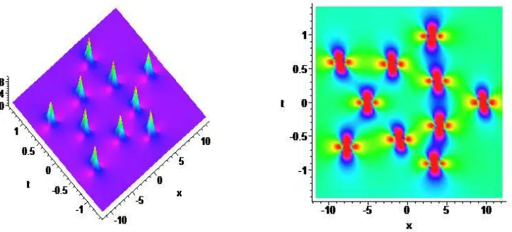
Whenn= 2, we construct the 2nd-order rogue waves under the assumptiond1 =eic1(s0+s1ε), d2 = e−ic1(s0+s1ε), s

0 = 0 from Theorem 3. An explicit form ofq[2] is constructed as q[2] =ceia(x+t(a2−6c2))B

C. (28)

Here, B and C are two degree 6 polynomials in x and t, which are given in appendix A. From Figure 1 (right), one finds that under the assumption d1 = 1, d2 = 1, or equivalently s0 = s1 = 0, the second-order rational solution admits a single high maximum at the origin.

By suitably adjusting the parametera one could control the decaying rate of the profile in the (x, t)-plane. This is a fundamental pattern. Furthermore, as is shown in Figure 6, when taking

d1 6= 1 andd2 6= 1, the large peak of the 2nd rogue wave is completely separated and forms a

set of three first-order rational solution for sufficiently larges1 meanwhile s0 = 0, and actually

forms an equilateral triangle.

When n = 3, and set d1 =eic1(s0+s1ε+s2ε 2

) _{and d}

2 =e−ic1(s0+s1ε+s2ε 2

)_{, then Theorem 3 yields}

s1 =s2 = 0, we have

q[3] = L1

L2 ei(32x−

45

8t). (29)

Here, L1 andL2 are two degree 12 polynomials in xand t, which are given in appendix B. This

is the fundamental pattern of the 3rd-order rogue wave, which is plotted in Figure 2(left) with a different value of a.

In general, Theorem 3 provides an efficient tool to produce analytical forms of higher-order rogue waves of the complex mKdV equation. Actually, we have also constructed the analytical formulas for 4th, 5th and 6th -order rogue waves. However, because of their long expressions describing these solutions, we do not present them here but would provide upon request. The validity of all these higher-order rogue waves has been verified by symbolic computation. Ac-cording to the explicit formulae of the nth-order rogue waves under fundamental patterns, we find that their maximum amplitude is (2n+ 1)2_c2_{(n = 1,2,3,4,5,6) by setting x= 0 andt= 0}

in _|q[n]_|2_{, and the height of the asymptotic plane is c}2_{, which is the same as that of the rogue}

wave of the NLS equation. This fact can be easily verified through Figs.(1-3). All figures in this paper are plotted based on these explicit analytical formulas of the solutions. Once the explicit analytical higher-order rogue waves are known, our next aim is to generate and understand underlying the dynamics of the obtained different patterns by suitably selecting the value ofsi .

4. Results and discussion

The above discussion is a clear manifestation of the evolution of the higher-order rogue waves from the Taylor expansion of the degenerate breather solutions. A brief discussion about the generating mechanism of higher-order rogue waves from the nonlinear evolution equation has already been reported by [40]. For our purpose now, we customize our discussion only up to 6th-order rogue waves, since higher-order rogue waves are difficult to construct owing to the extreme complexity and tedious mathematical calculations. It is quite obvious from our nu-merical analysis that the choice of parameters such as d1 and d2 actually do generate three

different basic patterns of rogue wave solutions. Let us discuss these patterns now.

Fundamental patterns: When, e.g. d1 =d2 = 1, or equivalentlysi = 0 (i= 0,1,2,· · · , n−1) in q[n]_{, the rational solutions of any order n have a similar structure. In addition, there are}

n(n+1)

2 −1 local maxima on each side of the line at t= 0. Starting from ∞, before the central

optimum high amplitude, there is a sequence of peaks with gradual increase in height. Here, one can observe that the number of first peaks is n, then there is a row of n₋1 symmetric peaks with respect to timet as shown in Figs. (1-3) for 6 rogue waves.

There are only two parameters a and c in the explicit forms of the rogue waves under fundamental patterns. It is a challenge problem to illustrate analytically the role of a and

c in the control of the profile for the higher-order RWs due to the extreme complexity of the explicit forms of the nth-order RWs (n_≥2). So, we only study this problem for the first-order RW _|q[1]_|2_{. To this end, we introduce a method, i.e., the contour line method, to analyze the}

contour profile of the red bright spots in the density plot of Fig. 4, which intuitively shows the localization characters such as length and width of the RW. On the background plane with height c2_{, a contour line of|q}[1]_|2 _{with c= 1 is a hyperbola}

x2₋12tx+ 6ta2x+ 36t2₋72t2a2+ 9t2a4₋ 1

4 = 0, (30)

which has two asymptotes

l1 :x= (6−3a2−6a)t, l2 :x= (6−3a2+ 6a)t, (31)

and two non-orthogonal axes:

major axis :t = 0, imaginary axis(l3) :x= (6−3a2)t. (32)

There are two fixed vertices: P1 = (0,0.50), P2 = (0,−0.5) on (t, x) plane of all value of a.

Here, l3 is also a median of one triangle composed of above two asymptotes and a parallel line

of x-axis except t = 0. We combine the density plots and the above three lines in Fig.4 with different values of a. At height c2_{+ 1, a contour line of |q}[1]|2

with c = 1 is given by a quartic polynomial

x4_{+ (12a}2_−24)tx3_{+ (}5

2 + (216−144a

2 _{+ 54a}4_)t2_)x2_{+ ((−864 + 432a}2_−216a4_{+ 108a}6_)t3

+(15a2_{−30)t)x+ (1296 + 648a}4_{+ 81a}8_)t4_{+ (90−144a}2_{+ (}45 2)a

4_)t2₋ 7

16 = 0, (33)

which has two end points P3 = (− √

7 12a,

(−2+a2 )√7

4a ) and P4 = ( √

7 12a,−

(−2+a2 )√7

4a ) along t-direction. Moreover, there are two fixed points expressed byP5 = (0,

q −1−4c2

+4√c2 (c2

+1)

2c |c=1) = (0,0.41),

P6 = (0,−

q

−1−4c2₊₄√_c2_(c2₊₁₎

2c |c=1) = (0,−0.41) on (t, x) plane of all value of a. At height c2

2, a

contour line of _|q[1]_|2 _{with c= 1 is also given by a quartic polynomial} x4_{+ (12a}2_−24)tx3_{+ ((216−144a}2_{+ 54a}4_)t2₋7

2)x2 + ((−864 + 432a2−216a4+ 108a6)t3

+(₋21a2_{+ 42)t)x+ (1296 + 648a}4_{+ 81a}8_)t4_{+ (−126 + 288a}2₋63 2a

4_)t2₊ 17

16 = 0, (34)

which is defined on interval [- 1 12a,

1

12a] of t. For this contour line, there are four fixed points: (0,1.78),(0,0.58),(0,₋0.58),(0,₋1.78) on (t, x) plane of all value of a. Two centers of valleys of_|q[1]_|2 _{given byP}

7 = (0, √

3

2c), P8 = (0,− √

3

2c), which are independent with the value ofa. Fig.5 are plotted for above contour lines with different values of a= 1.5,2,2.5.

Based on the above analytical results, we could define the length and width of the rogue wave, which are two crucial characters of a doubly localized wave-RW. Because the contour line of RW on the background plane is not a closed curve, so we can not define a length for RW on this plane. However, set d be a positive constant, the contour line at height c2_{+d is}

closed. Herec2_{+d <9c}2_{, or equivalentlyd <}√_8c2_{because the max amplitude of the first-order}

RW (_|q[1]_|2_{) is 9c}2_{. Without loss of generality, and considering a recognizable height from the}

asymptotic plane, we set d = 1 as before. We can use the length of the area surrounded by the contour line at height c2_{+ 1 as the length of the first-order RW. The length-direction is}

defined by l3, the width-direction is orthogonal to it. The reasons for this choice are : 1) l3

passes through P3 and P4; 2) l3 is parallel to the tangent line of hyperbola at two vertices; 3) l3 is parallel to the tangent line of the contour line at P5 and P6. Let k3 be the slope of l3. So

the length of the first-order RW is the distance of P3 and P4, i.e.,

dL= √

7 6a

p

1 + (k3)2 =

√ 7 6a

p

1 + (6₋3a2₎2_{. (35)}

The width is defined as the projection of line segment P7P8 at width-direction, which is

ex-pressed by

dW =

√ 3

p

1 + (k3)2

=

√ 3

p

1 + (6₋3a2₎2. (36)

dLanddW are plotted in figure 6 with fixedc= 1, which shows that the length is decreased with

a whena _∈(0,√2) and is increased witha when a >√2. However, the width has an opposite increasing or decreasing trend with respect to a. When a =√2, the profile of first-order RW is parallel to the t-axis, then the length reaches to its minimum, and the width reaches to its maximum. This is the first role ofain the control of the RW. Moreover, we know from k3 that

the increase of a results in the rotation of RW in the clockwise direction. This is the second role of a.

In above discussion for the role of a, we have set c = 1. If c ₆= 1, it is a more interesting and complicated case, which can be studied as above by using contour line method. To save the space, we shall provide corresponding results without explanation, which can be done by a similar way as above. Under this case, two asymptotes of the contour line of first-order RW |q[1]_|2 _{at height c}2

major axis :t= 0, imaginary axis(cl3) :x= (6c2−3a2)t. (37)

In other word, slope is k3c = 6c2 − 3a2. Two vertices of the hyperbola are P1 = (0,₂1_c)

and P2 = (0,−₂1_c) on (t, x) plane. For contour line at height c2 + 1, two end points are P3 = (−

√ 8c2

−1 12ac2 ,

(−2c2 +a2

)√8c2 −1

4ac2 ) and P4 = ( √

8c2 −1 12ac2 ,−

(−2c2 +a2

)√8c2 −1

4ac2 ) along t direction. So the

length of the first-order RW is

dcL = √

8c2₋₁

6c2_a

p

1 + 9(₋2c2 _+a2₎2_{, (38)}

and the width of the first-order RW is

dcW = √

3

c

1

p

1 + 9(₋2c2_+a2₎2, (39)

which are plotted in Figure 7. These pictured show visually the role of a and c in the control of the first-order RW. For a given value of a, dcL has two extreme points with respect to c. However, for a given value of c, dcL has one extreme point with respect to a. The slope k3c shows that the increasing ofa and cresults in the rotation of the first-order RW with different direction. Note that a =√2c is a line of points for extreme value. Under this condition, the profile of first-order RW is parallel to the t-axis, and the minimum of the length is √4a2

−1 3a3 , the

maximum of the width is √3

c .

Triangular patterns: The triangular structure can be obtained by choosing the first non-trivial coefficient s1 ≫ 1, while the rest of the values are assumed to be zero. It can be seen

from Figs. (8-10) that the n-th order rational solutions have n(n₂+1) peaks of equal height with a structure of equilateral triangular type having n peaks at each edge.

Ring patterns: One can observe the ring structure/pattern when n _≥ 3 and the principle coefficient for n-th order rational solution when sn₋1 ≫ 1, while the remaining coefficients si are all zero. The rational solutions consist of the outer circular shell of 2n₋1 first-order rational solutions, while the center is an order (n₋2) rational solution of the fundamental patterns as portrayed in Figs. (11-12). The center order-(n₋2) rogue wave can be decomposed further into different lower-order patterns according to the (n₋2)-reduction rule of order by setting one of si (i = 0,1,2, . . . , n−3) to non-zero, which are plotted in Figs. (13-15). For example, the center order-4 rogue wave of the 6-th rogue wave has a fundamental pattern (Figure 12 (right)), a ring plus a fundamental pattern (Figure 14 (right)) or triangular pattern ((Figure 15 (right))) of 2nd-order rogue wave, a triangular pattern (Figure 15 (left)). We call these forms

as standard decomposition of the rogue wave. This structure is similar to the so-called “wave clusters” as reported in [50].

Another interesting fact worth mentioning here is that the profiles of higher-order rogue wave are actually a complicated combination of above three basic patterns: “fundamental” pattern, “ring” pattern and “triangular” pattern, which can provide further interesting patterns of the rogue waves. This can be achieved by suitably selecting the different values ofsi. In particular, one can generate multi-ring structures but these rings do not possess 2n-1 peaks and also do not satisfy the rule of (n-2)-reduction of order as mentioned earlier in the case of ring pattern formation. Thus, we call these formations as non-standard decomposition of the rogue waves. Figures (16-20) represent a few examples of this kind of special ring structures. One common feature, which we observed from these examples, is the appearance of at least two ring patterns with the same number of peaks. It should be noted that the center-most profile of Figure 18 (left) is a fundamental pattern of a 2nd-order rogue wave, which clearly shows that Figure 18 (left) is not a complete decomposition of the 6-th order rogue wave. On the other hand, Figure 18 (right) presents the complete decomposition. To arrive to a better understanding of the non-standard decomposition, we provide the distribution of peaks in Table 1. From Figure 19 (left), it can also be observed the occurrence of two ring patterns with a single inner peak, however, the inner ring consists of 5 triangular patterns. So, the distribution of peaks is 5 + 3_×5 + 1.

In spite of having different structures, all types of rogue wave solutions possess certain com-monality as follows: The total number of peaks admitted by n-th order solutions is n(n₂+1) in terms of a complete decomposition pattern. These structures actually depend on the choice of the free parameters. Among all parameters, the principle coefficientsn−1 is accountable for the

formation of a ring structure. The first non-trivial coefficient s1 is responsible for the

evolu-tion of a triangular structure. Furthermore, to see difference between the RWs of the complex mKdV and the NLS clearly, we use the first-order RW ( [40]) of the NLS, i.e.,

q_{N LS}[1] =c2A˜−32c

2_{((−x+ 2at)}2_−4c2_t2_{) + 8}

˜

A ,

˜

A = (4c2x2₋16c2xta+16t2(c4+c2a2)+1)2. (40) to calculate the contour lines at heights c2 and c2 + 1, and to calculate the length, width by the same procedure we have used in complex mKdV. Here the NLS equations is in the form of

iqt+qxx+ 2|q2|q= 0. (41) Similar to the contour line method of the complex mKdV, we get the slope of the imaginary axis of the hyperbola formed by a contour line of the_|q_{N LS}[1] _|2 _{on background plane with a height} c2_:k

3cN LS = 2a, and the length of the RW

dcLN LS = 1 2c2

p

(₋1 + 8c2_{)(1 + 4a}2_{), (42)}

and the width of the RW

dcW N LS =

√ 3

c √1 + 4a2. (43)

The dynamical evolution of the first-order RW _|q_{N LS}[1] _|2 _{of the NLS are plotted in Fig. 21,}

contour lines at heightsc2 _andc2_{+ 1 of the first-order RWs of the complex mKdV and the NLS}

are plotted in Fig. 22. These pictures and analytical formulae of length and width show that, for the first-order RWs of the complex mKdV and the NLS, they are very similar to each other apart from a remarkable tilt with respect to the axes and a remarkable shortening of length of them with same values of a and c. In other words, the inclusion of third-order dispersion and

time-delay correction is responsible for a strong rotation and a strong compression effects in the first-order RW of the complex mKdV equation. In particular, ifa = 0,_|q[1]_{N LS|}2 is still a RW, but |q[1]_|2 _{of the complex mKdV is a soliton traveling along l}

3 which is no longer doubly-localized

inx and t directions.

In terms of applications, the investigation of the above investigated higher-order RW solutions will be useful to understand the generation of high-power waves and their possible splitting, etc. As we have discussed earlier, very recently, using the non-slowly varying envelope approximation (SVEA), the complex mKdV equation has been derived and the generation of few-cycle optical pulses have been reported [42, 43]. In addition, it has been pointed out that these type of few-cycle optical pulses require no phase matching (a main issue in nonlinear optics), which makes a strong contrast and provides an interesting aspect when compared with the longer pulses derived by using the SVEA method. From these recent studies it is also interesting to note that these type of few-cycle optical pulses are very similar to the generation of high-power and very short RW type ultra-short pulses. For example, in nonlinear photonic crystal fibre, the above waves may be connected to the generation of few-cycle optical pulses which will be useful to realize the so-called supercontinuum generation. This type of white light continuum coherence source will find a range of applications in optical coherence tomography, optical meteorology, wavelength division multiplexing, fluorescence microscopy, flow cytometry, atmospheric sensing, etc. [1, 42, 43].

5. Conclusions

In this paper, we applied the DT to construct the higher-order RW-type rational solutions as well as the evolution of rogue waves for the complex mKdV equation. Based on detailed numerical and analytical investigations, we classified the higher-order RWs with respect to their intrinsic structure. We use the contour line method, for the first time to the best of our knowledge, to define the length and width of the first-order RW, and then provide their analytical formulae related to two parameters a and c. We illustrate clearly, by analytical formulas and figures, that the differences between the first-order RWs of the mKdV and the NLS are mainly due to strong rotation as well as strong compression effects. Furthermore, we observed that there are three principle types, namely, fundamental pattern, ring pattern, and triangular pattern. The composition of these three principle patterns is mainly because of higher-order rogue waves. We also provided several further new patterns of the higher-order RWs of this model. The ring patterns obtained in this paper are similar to the “atom” structure reported in [50]. This explains the generalization and evolution of higher-order RWs in terms of the solution. On the other hand, by changing the free parameters in the DT, we have also constructed more complicated (and interesting) structures. We deduced from our stimulated examples in Figs. 16-20 that the non-standard decomposition deserves further studies because there are presently unknown rules of the decomposition. Applying our construction of RW solutions to different completely integrable nonlinear evolution equations, it is interesting to investigate some analogues between the evolution and decomposition of higher-order RWs of these different integrable equations. It is essential to find further conserved quantities for the kind of solutions. These studies may help us for better understanding of the occurrence of deep ocean waves with large amplitude as well as the generation of few-cycle optical pulses emitted by high-power lasers which are used for the recently invented supercontinuum generation sources, etc.

If we compare our results with the work in [38] on the rogue wave solutions of the complex mKdV, our results have following advantages and developments:

• Our method is considerably simpler as well as more systematic. From Theorem 3, one can directly obtain the higher-order RWs without calculating eigenfunctions ψ₁[i] and

φ[₁i](i= 0,1,2,3) as in [38].

• We applied the contour line method to find the analytical description of the length and width of the first-order RW of the complex mKdV and the NLS equation. We illustrated clearly, using suitable analytical formulae and figures, that the differences between the first-order RWs of the mKdV and the NLS are due to a strong rotation and a strong compression effects. Note that, settinga = 0,_|q[1]_|2 _{reduces to a soliton on a background}

plane at height c2_{, but |q}[1]

N LS|2 can not.

• We proposed and proved a convenient way to control the patterns and evolutions of the rogue wave by standard and non-standard decomposition with suitable choices of si. • We generated interesting patterns for 4th,5th and 6th rogue waves.

With respect to the future research in this exciting area, we shall apply the contour line method to the first-order RW of the different NLS type equations. For the higher-order rogue waves, because the degree of polynomials in its explicit form is more than 4, it is not easy to get the analytical expressions of the asymptotes for its contour lines in general. Thus, how to get the analytical results on their length and width is an interesting, difficult and important problem, which deserves further study.

Acknowledgments

This work is supported by the NSF of China under Grant No.11271210 and the K. C. Wong Magna Fund in Ningbo University. J.S. He thanks sincerely Prof. A.S. Fokas for arranging the visit to Cambridge University in 2012-2013 and for many useful discussions. KP acknowledges DST, NBHM, CSIR and IFCPAR, Government of India, for the financial support through major projects. RE acknowledges M. K´eray for patient encouragement and is also grateful to NSF, Hungary (OTKA, Ref. No.K83133). This work has been partially supported by The University of Sheffield’s MSRC Visitor Grant. We thank editorial board member for his/her suggestions on our submission which has improved the clarity of the paper.

References

[1] G.P. Agrawal,“Nonlinear Fiber Optics”, 5th edition (Academic Press, San Diego, CA, 2012). [2] B.A.Malomed,“Soliton management in periodic systems”(Springer,New Yrok, 2006)

[3] S.K. Turitsyn, B.G.Bale, M.P.Fedoruk, Phys.Report521(2012)135. [4] D. J. Korteweg, and G. de Vries, Phil. Mag.39(1895)422 .

[5] N. J. Zabusky and M. D. Kruskal, Phys. Rev. Lett.15(1965)240. [6] V.E Zakharov and A.B Shabat, Sov. Phys. JETP34(1972)62.

[7] L. F. Mollenauer, R. H. Stolen, and J. P. Gordon, Phys.Rev.Lett.45(1980)1095. [8] A Hasegawa and F D Tappert, Appl. Phys. Lett.23(1973)142 .

[9] D.H. Peregrine, J. Austral. Math. Soc. B25(1983)16.

[10] D. R. Solli, C. Ropers, P. Koonath,B. Jalali, Nature(London) 450(2007)1054. [11] D. R. Solli, C. Ropers, B. Jalali, Phys. Rev. Lett.101(2008) 233902.

[12] J. M. Dudley, G. Genty and S. Coen, Rev. Mod. Phys. 78(2006)1135; J. M. Dudley, G. Genty, F. Dias, B. Kibler, N. Akhmediev, Opt. Express17(2009) 21497.

[13] A. N. Ganshin, V. B. Efimov, G.V. Kolmakov, L. P. Mezhov-Deglin, P.V. E. McClintock, Phys.Rev.Lett. 101(2008)065303.

[14] Yu. V. Bludov, V. V. Konotop,N. Akhmediev,Phys.Rev.A.80(2009)033610. [15] M.S. Ruderman,Eur. Phys. J. Special Topics185(2010 57.

[16] W.M.Moslem, P.K.Shukla, B.Eliasson, Euro. Phys. Lett.96(2011)25002.

[17] R. H¨ohmann, U. Kuh, H.-J. Stockmann, L. Kaplan, E. J. Heller, Phys.Rev.Lett.104(2010)093901. [18] M. Shats, H. Punzmann, H. Xia,Phys.Rev.Lett.104(2010)104503.

[19] S.Vergeles,S.K.Turitsyn, Phys.Rev.E83(2011)061801(R).

[20] F. T. Arecchi, U. Bortolozzo, A. Montina, S. Residori, Phys.Rev.Lett.106(2011)153901

[21] A.Chabchoub, N.P.Hoffmann, N.Akhmediev, Phys. Rev. Lett. 106(2011)204502; J. Geophys. Res. 117(2012)C00J02.

[22] B. Kibler, J. Fatome, C. Finot, G. Millot, F. Dias, G. Genty, N. Akhmediev,J. M. Dudley, Nature Phys.6(2010)790.

[23] N. Akhmediev, A. Ankiewicz, M. Taki,Phys. Lett. A373(2009)675.

[24] A. Ankiewicz, J. M. Soto-Crespo, N. Akhmediev, Phys. Rev. E.81(2010)046602. [25] J. M. Soto-Crespo, Ph. Grelu, N. Akhmediev, Phys.Rev. E84(2011)016604. [26] A.Ankiewicz, N.Akhmediev, J. M. Soto-Crespo, Phys. Rev. E.82(2010)026602. [27] U. Bandelow, N. Akhmediev , Phys. Rev. E86(2012)026606.

[28] P. Dubard, V.B. Matveev, Nat. Hazards. Earth. Syst. Sci.11(2011)667.

[29] Y. Ohta, J. K. Yang, Proc. R. Soc. A468(2012)1716-1740; Phys.Rev.E86(2012)036604.

[30] S.W.Xu, J.S. He, L.H.Wang, J. Phys. A44 (2011) 305203; Y.Y.Wang, J.S.He,Y.S. Li, Commun.Theor. Phys.56(2011) 995-104; Y.S.Tao ,J.S. He, Phys. Rev. E.85(2012) 026601; S.W.Xu, J.S.He,J. Math. Phys. 53(2012) 063507; J.S.He, S.W.Xu, K. Porsezian, J. Phys. Soc. Jpn.81(2012) 124007; J.S. He, S.W. Xu, K. Porsezian, J. Phys. Soc. Jpn.81(2012) 033002; S. W. Xu, J. S. He, L. H. Wang, Euro. Phys. Lett.97 (2012) 30007; J.S.He, S. W.Xu, K. Porsezian, Phys.Rev.E86(2012)066603; C.Z.Li, J.S.He, K.Porsezian, Phys.Rev.E87(2013)012913; L. H. Wang, K. Porsezian,J. S. He, Phys.Rev.E 87(2013)053202; S.W. Xu, K. Porsezian, J. S. He, Y. Cheng, Phys.Rev.E88(2013)062925.

[31] G.G.Yang, L.Li, S.T.Jia, Phys.Rev.E88(2012) 046608. [32] B.L.Guo, L.M.Lin,Chin.Phys.Lett.28(2011) 110202.

[33] F. Baronio, A. Degasperis, M. Conforti1,S. Wabnitz, Phys.Rev.Lett. 109(2012) 044102. [34] Z.Y. Qin, M.Gu, Phys.Rev.E 86(2012) 036601.

[35] L.C.Zhao, J. Liu, Phys. Rev.E87 (2013)013201.

[36] M.Taki,A.Mussot, A. Kudlinski, E. Louvergneaux, M. Kolobov, M. Douay, Phys. Lett.A374(2010)691. [37] S.H.Chen, L.Y.Song, Phys.Rev.E87(2013)032910.

[38] Q.L.Zha, Phys.Scr.87(2013)065401.

[39] L. J. Li, Z. W. Wu, L. H. Wang, J. S. He, Annals of Physics 334(2013)198.

[40] J.S.He, H.R. Zhang, L.H. Wang, K. Porsezian,A.S.Fokas,Phys.Rev.E87(2013)052914.

[41] M.J. Ablowitz and P.A. Clarkson, “Solitons, Nonlinear Evolution Equations and Inverse Scattering” (Cambridge University Press, Cambridge, NY, 1991).

[42] H.Leblond,H.Triki,F.Sanchez and D.Mihalache, Optics Communications 285(2012)356. [43] H.Leblond and D.Mihalache, Romanian Reports in Physics63(2011)1254.

[44] G. Neugebauer and R. Meinel, Phys. Lett. A. 100(1984)467.

[45] Y. S. Li, X. S. Gu, M. R. Zou, Acta Mathematica Sinica (New Series)3(1985)143. [46] V. B. Matveev, M. A. Salle,Darboux transformations and solitons(Springer, Berlin,1991) [47] C. H. Gu, Z. X. Zhou, Lett. Math. Phys.13(1987)179.

[48] C. H. Gu, H. S. Hu and Z. X. Zhou, Darboux Trasformations in Integrable Systems (Dortrecht: Springer)(2006).

[49] J. S. He, L. Zhang, Y. Cheng and Y. S. Li, Science in China Series A: Mathematics.12(2006)1867. [50] D. J. Kedziora, A. Ankiewicz, and N. Akhmediev, Phys. Rev. E84(2011)056611.

Table 1. _{Distribution of peaks on rings by non-standard decomposition}

Order Distributions of peaks on rings (L=Left,R=Right)

4 5+5(Fig.12)

5 7+7+1(Fig.13L) 5+5+5(Fig.13R)

Appendix A:In eq.(28), L1 are L2 are given by

B := 2239488a4c14t6+ 46656a12c6t6+ 2985984c18t6+ 559872a8c10t6

+746496a6c10t5x+ 93312a10c6t5x₋1492992a4c12t5x₋186624a8c8t5x

+1492992a2c14t5x₋2985984c16t5x+ 1244160c14t4x2₋248832a6c8t4x2

−995328a2c12t4x2+ 622080a4c10t4x2+ 77760a8c6t4x2₋276480c12t3x3

+34560a6c6t3x3₋124416a4c8t3x3+ 248832a2c10t3x3+ 34560c10t2x4

+8640a4c6t2x4₋27648a2c8t2x4+ 1152a2c6tx5 ₋2304c8tx5+ 64c6x6

−331776c6a6t4₋518400c12t4+ 155520c8a4t4₋11664c4a8t4+ 290304c10t3x

−15552c4_a6_t3_{x+ 103680c}8_a2_t3_x−176256c6_a4_t3_x−58752c8_t2_x2_−6912c6_a2_t2_x2

−7776c4a4t2x2+ 4992c6tx3₋1728c4a2tx3₋144c4x4+ 124416ac10s1t3

+31104a5c6s1t3−165888a3c8s1t3 + 20736a3c6s1t2x−41472ac8s1t2x

+3456ac6s1tx2−18000c6t2−1620c2a4t2−1080c2a2tx+ 5616c4tx−180c2x2

+864c4as1t+ 144c4s21+ 45 +i(2985984ac14t5+ 1492992a5c10t5

+186624a9c6t5₋497664a5c8t4x+ 995328a3c10t4x₋1990656ac12t4x

+248832a7c6t4x₋331776a3c8t3x2+ 124416a5c6t3x2+ 497664ac10t3x2

−55296ac8t2x3+ 27648a3c6t2x3+ 2304ac6tx4+ 207360c8at3₋31104c4a5t3

−13824c6at2x₋20736c4a3t2x₋3456c4atx2 + 20736c8s1t2 −41472a2c6s1t2

+5184a4c4s1t2+ 3456a2c4s1tx−6912c6s1tx+ 576c4s1x2−2160ac2t+ 144s1c2)

and

C := 2239488a4c14t6+ 2985984c18t6+ 46656a12c6t6+ 559872a8c10t6

+746496a6c10t5x₋1492992a4c12t5x₋186624a8c8t5x₋2985984c16t5x

+93312a10c6t5x+ 1492992a2c14t5x+ 1244160c14t4x2₋995328a2c12t4x2

+622080a4c10t4x2+ 77760a8c6t4x2₋248832a6c8t4x2 + 248832a2c10t3x3

+34560a6_c6_t3_x3_−124416a4_c8_t3_x3_−276480c12_t3_x3 _−27648a2_c8_t2_x4

+8640a4c6t2x4 + 34560c10t2x4 ₋2304c8tx5+ 1152a2c6tx5+ 64c6x6

+995328c10a2t4+ 279936c8a4t4₋82944c6a6t4+ 3888c4a8t4₋269568c12t4

+124416c10t3x+ 5184c4a6t3x₋51840c6a4t3x₋145152c8a2t3x

−17280c8t2x2₋6912c6a2t2x2+ 2592c4a4t2x2+ 384c6tx3

+576c4a2tx3+ 48c4x4 ₋165888a3c8s1t3+ 124416ac10s1t3

+31104a5c6s1t3+ 20736a3c6s1t2x−41472ac8s1t2x+ 3456ac6s1tx2

+20016c6t2+ 972c2a4t2+ 6912c4a2t2+ 648c2a2tx₋2448c4tx+ 108c2x2

−2592c4as1t+ 144c4s21+ 9.

Appendix B:In eq.(29), L1 are L2 are given by

L1 :=−4939273445868140625t12−545023276785450000t11x−388407392651700000t10x2

−34025850934560000t9x3₋12374529519456000t8x4₋841946352721920t7x5

−204871837925376t6x6 ₋10322713903104t5x7₋1860148592640t4x8₋62710087680t3x9

−8776581120t2x10₋150994944tx11₋16777216x12+ 2300237292280725000t10

+500080291038360000t9x+ 178207653254544000t8x2+ 20160748631347200t7x3

+4231975119851520t6x4+ 253682249269248t5x5+ 40317552230400t4x6+ 880347709440t3x7

+141203865600t2_x8_{−1447034880tx}9_{+ 75497472x}10_{+ 257120426548112400t}8

−88521031030049280t7x₋1841385225323520t6x2₋617799343104000t5x3

−88747774156800t4x4₋8252622766080t3x5₋200693514240t2x6+ 1415577600tx7

+235929600x8+ 12647412412496640t6+ 42148769126400t5x₋2996161228800t4x2

−15902996889600t3x3+ 313860096000t2x4₋8139571200tx5+ 707788800x6

−149676507590400t4+ 2148738969600t3x₋1622998425600t2x2+ 31186944000t3x

−928972800x4₋95215564800t2+ 21598617600tx₋464486400x2+ 58060800

+i(₋6540279321425400000t11₋601404995073600000t10x₋423057306879360000t9x2

−29901007761408000t8x3₋10648770814771200t7x4₋552411244265472t6x5

−130559642173440t5x6 ₋4494741995520t4x7₋779700142080t3x8₋13589544960t2x9

−1811939328tx10₋303419904173280000t9+ 263517097430016000t8x

+29562711599923200t7x2+ 7820253397647360t6x3+ 799710056939520t5x4

+58500443013120t4_x5_{+ 5243865661440t}3_x6_{+ 40768634880t}2_x7_{+ 6794772480tx}8

+10822374648023040t7₋15805156998758400t6x₋366298181959680t5x2

+157459297075200t4x3₋6736379904000t3x4₋249707888640t2x5+ 16986931200tx6

+2321279745269760t5₋164322282700800t4x+ 7849554739200t3x2₋700710912000t2x3

+38220595200tx4+ 4992863846400t3₋967458816000t2x₋33443020800tx2₋8360755200t)

L2 := 4939273445868140625t12+ 545023276785450000t11x+ 388407392651700000t10x2

+34025850934560000t9x3+ 12374529519456000t8x4+ 841946352721920t7x5

+204871837925376t6x6+ 10322713903104t5x7+ 1860148592640t4x8

+62710087680t3x9+ 8776581120t2x10+ 150994944tx11+ 16777216x12

+1671541529351175000t10₋201221180459640000t9x+ 29583374214960000t8x2

−8646206984294400t7x3₋205872145551360t6x4₋102185078390784t5x5

−5361951375360t4x6₋141416202240t3x7₋16349921280t2x8+ 2202009600tx9

+25165824x10_{+ 214192109547903600t}8_{+ 4346367735790080t}7_x

+3783154346910720t6x2₋1075635551969280t5x3+ 40942170316800t4x4

+1840480911360t3x5+ 84333035520t2x6+ 849346560tx7+ 141557760x8

+3537485306138880t6+ 789853361080320t5x+ 130057245388800t4x2

−11222478028800t3x3+ 402245222400t2x4₋4034396160tx5+ 613416960x6

+90779142700800t4₋6216180019200t3x₋269186457600t2x2+ 11988172800tx3

+221184000x4+ 213178521600t2 ₋5009817600tx+ 199065600x2+ 8294400.

Figure 1. (Color online) Fundamental pattern of the rogue wave. (a) The left figure is the evolution of _|q[1]_|2 (1st-order rogue wave) with specific parameters a = 1.5, c = 1, s0 = 0.

(b) The right figure is_|q[2]_|2 (2nd-orderrogue wave) with specific parametersa= 1.44, c= 1, s0= 0, s1= 0.

Figure 2. (Color online) Fundamental pattern of the rogue wave. (a) The left figure is the evolution of _|q[3]_|2 _{(3rd-order rogue wave) with specific parameters a = 1.4, c =}

1, s0 = 0, s1 = 0, s2 = 0. (b) The right figure is |q[4]|2 (4th-order rogue wave) with specific

parametersa= 1.48, c= 1, s0 = 0, s1 = 0, s2 = 0, s3 = 0.

Figure 3. (Color online) Fundamental patterns of the rogue waves. (a) The left figure is the evolution of_|q[5]_|2 (5th-order rogue wave) with specific parameters a= 1.5, c= 1, s0 =

0, s1 = 0, s2 = 0, s3 = 0, s4 = 0. (b) The right figure is |q[6]|2 (6th-order rogue wave) with

specific parametersa= 1.5, c= 1, s0 = 0, s1 = 0, s2 = 0, s3 = 0, s4 = 0, s5 = 0.

Figure 4. (Color online) The density plots of the first-order rogue wave _|q[1]_|2 with c= 1 and different values ofa. From left to right,a= 1.5,2,2.5 in order. Here red (solid) and blue (dot) lines are plotted for two asymptotes of contour lines at height c2, green (dash) line is plotted for a median of one triangle composed of above two asymptotes and a parallel line of

x-axis exceptt= 0. Two fixed pints are located at (0,0.5) and (0,₋0.5) in three panels.

Figure 5. (Color online) Contour lines of the first-order rogue wave with c = 1 and

a= 1.5(red, solid), 2(dash,green), 2.5(dot, blue). From left to right, panels are plotted for contour lines of _|q[1]_|2 _{at height c}2 _{(on asymptotic plane), c}2 _{+ 1, c}2_{/2 in order. There are}

fixed points located at (0,0.50) and (0,₋0.50) in the left panel, (0,0.41) and (0,₋0.41) in the middle panel, (0,1.78) and (0,0.58), (0,₋0.58) and (0,₋1.78) in the right panel.

Figure 6. (Color online) The length (red, solid) and the width (dash, green) of the first-order RW_|q[1]_|2 with fixed c= 1. Note a=√2 is an extreme point of dL and dW.

Figure 7. (Color online) The length(left) and width(right) of the first-order RW_|q[1]_|2 with two parametersaand c.

Figure 8. (Color online) Triangular pattern of the 2nd- and 3rd-order rogue waves. The left panel is a density plot of_|q[2]_|2(2nd-orderrogue wave) witha= 1.44, c= 1, s0= 0, s1= 100.

The right panel is a density plot of_|q[3]_|2 (3rd-order rogue wave) witha= 1.44, c= 1, s0 =

0, s1= 100, s2 = 0.

Figure 9. (Color online) Triangular pattern of the 4th-order and 5th-order rogue waves. The left panel is a density plot of_|q[4]_|2 (4th-order rogue wave) with a= 1.46, c= 1, s0 =

0, s1= 100, s2 = 0, s3 = 0, the right panel is a density plot of|q[5]|2 (5th-order rogue wave)

witha= 1.5, c= 1, s0= 0, s1= 100, s2 = 0, s3 = 0, s4 = 0.

Figure 10. (Color online) Triangular pattern of the 6th-order rogue wave. (a) The left figure is the evolution of_|q[6]_|2 (6th-orderrogue wave) and (b)the right figure is the corresponding density plot witha= 1.5, c= 1, s0= 0, s1= 100, s2 = 0, s3 = 0, s4 = 0, s5 = 0.

Figure 11. (Color online) Standard circular decomposition of the rogue wave: inner peak surrounded by ring pattern. The left panel is a density plot of_|q[3]_|2 _{(3rd-orderrogue wave)}

with a = 1.4, c = 1, s0 = 0, s1 = 0, s2 = 1000, the right panel is a density plot of |q[4]|2

(4th-order rogue wave) witha= 1.48, c= 1, s0 = 0, s1 = 0, s2 = 0, s3 = 1000.

Figure 12. (Color online) Standard circular decomposition of the rogue wave: a ring pattern with inner 3rd (left) and 4th (right) fundamental patterns. The left panel is a density plot of |q[5]_|2 (5th-orderrogue wave) witha= 1.5, c= 1, s0 = 0, s1 = 0, s2 = 0, s3 = 0, s4 = 100000,

the right panel is a density plot of _|q[6]_|2 (6th-order rogue wave) with a= 1.5, c = 1, s0 =

0, s1= 0, s2= 0, s3= 0, s4 = 0, s5 = 100000000.

Figure 13. (Color online) Standard circular decomposition of the 4th and 5th rogue waves. The left panel is a density plot of_|q[4]_|2 _{(4th-order rogue wave) with a= 1.45, c= 1, s}

0 =

0, s1= 100, s2 = 0, s3 = 10000000 which is decomposed into an outer ring with an inner 2nd

triangular pattern, the right panel is a density plot of _|q[5]_|2_{(5th-order rogue wave) with}

a= 1.5, c = 1, s0 = 0, s1 = 100, s2 = 0, s3 = 500000, s4 = 100000000 which is decomposed

into an inner peak surrounded by two rings.

Figure 14. (Color online) Standard circular decomposition of the 5th and 6th rogue waves. The left panel is a density plot of _|q[5]_|2 (5th-order rogue wave) with a= 1.5, c = 1, s0 =

0, s1 = 50, s2 = 0, s3 = 0, s4 = 100000000 which is decomposed into a ring pattern with

an inner 3rd triangular pattern, the right panel is a density plot of_|q[6]_|2 (6th-order rogue wave) with a= 1.5, c= 1, s0 = 0, s1 = 0, s2 = 0, s3 = 0, s4 = 1000000, s5 = 100000000 which

is decomposed into two ring patterns plus an inner 2nd fundamental pattern.

Figure 15. (Color online) Standard circular decomposition of the 6th rogue wave. The left panel is a density plot of _|q[6]_|2 (6th-order rogue wave) with a = 1.5, c = 1, s0 = 0, s1 =

18, s2 = 0, s3 = 0, s4 = 0, s5 = 100000000 which is decomposed into a ring plus an inner 4th

triangular pattern, the right panel is a density plot of _|q[6]_|2 (6th-order rogue wave) with

a= 1.5, c= 1, s0 = 0, s1 = 0, s2 = 0, s3 = 7000, s4 = 0, s5 = 10000000 which is decomposed

into three rings.

Figure 16. (Color online) Non-standard circular decomposition of the 4th-rogue wave: two rings. (a) The left figure is the dynamical evolution of _|q[4]_|2 (4th-order rogue wave) and (b) the right figure is the corresponding density plot witha= 1.48, c= 1, s0 = 0, s1 = 0, s2 =

1000, s3 = 0.

Figure 17. (Color online) Non-standard circular decomposition of the 5th-rogue waves: two rings plus an inner peak (left) and three rings (right). The left panel is a density plot of |q[5]_|2 (5th-orderrogue wave) witha= 1.45, c= 1, s0 = 0, s1 = 0, s2 = 0, s3 = 10000, s4 = 0,

the right panel is a density plot of _|q[5]_|2 (5th-order rogue wave) with a= 1.46, c= 1, s0 =

0, s1= 0, s2= 1000, s3 = 0, s4 = 0.

Figure 18. (Color online) Non-standard circular decomposition of the 6th-rogue wave: two ring patterns with an inner 2nd fundamental pattern(left) and three rings(right). The left panel is a density plot of _|q[6]_|2 (6th-order rogue wave) with a = 1.5, c = 1, s0 = 0, s1 =

0, s2= 0, s3= 0, s4= 10000000, s5 = 0 , the right panel is a density plot of|q[6]|2 (6th-order

rogue wave) witha= 1.5, c= 1, s0= 0, s1= 15, s2= 0, s3= 0, s4 = 10000000, s5 = 0.

Figure 19. (Color online) Non-standard circular decomposition of the 6th-rogue wave: three rings plus an inner peak (left) and three rings (right). The left panel is a density plot of_|q[6]_|2

(6th-order rogue wave) witha= 1.5, c= 1, s0 = 0, s1 = 0, s2 = 10000, s3 = 0, s4 = 0, s5 = 0

, the right panel is a density plot of_|q[6]_|2 (6th-order rogue wave) with a= 1.5, c = 1, s0 =

0, s1= 0, s2= 0, s3= 1000000, s4 = 0, s5 = 100000000.

Figure 20. (Color online) Non-standard circular decomposition of the 6th-rogue wave: three rings. (a) The left panel is the dynamical evolution of _|q[6]_|2 _{(6th-order rogue wave)}

and (b) the right panel is the corresponding density plot with a = 1.5, c = 1, s0 = 0, s1 =

0, s2= 1000, s3 = 1000000, s4 = 0, s5= 100000000.

Figure 21. (Color online) The first-order rogue wave (_|q_{N LS}[1] _|2_{) of the NLS with a = 1.5}

and c = 1. The left panel is the dynamical evolution of _|q[1]_{N LS|}2 _{and the right panel is the}

corresponding density plot.

Figure 22. (Color online) Contour lines of the first-order rogue wave of the complex mKdV (_|q[1]_|2,red,solid) and NLS (_|q_{N LS}[1] _|2,green, dash) with a= 1.5 and c = 1. The left panel is plotted at heightc2 (on the asymptotical plane), the right panel is plotted at heightc2+ 1. Two lines have two common pints:(0,0.50),(0,₋0.50) in the left panel and (0,0.41),(0,₋0.41) in the right panel.