The Dynamic Chain Event Graph

White Rose Research Online URL for this paper:

http://eprints.whiterose.ac.uk/90184/

Version: Published Version

Article:

Barclay, LM, Collazo, RA, Smith, JQ et al. (2 more authors) (2015) The Dynamic Chain

Event Graph. Electronic Journal of Statistics, 9 (2). 2130 - 2169. ISSN 1935-7524

https://doi.org/10.1214/15-EJS1068

[email protected] https://eprints.whiterose.ac.uk/ Reuse

Unless indicated otherwise, fulltext items are protected by copyright with all rights reserved. The copyright exception in section 29 of the Copyright, Designs and Patents Act 1988 allows the making of a single copy solely for the purpose of non-commercial research or private study within the limits of fair dealing. The publisher or other rights-holder may allow further reproduction and re-use of this version - refer to the White Rose Research Online record for this item. Where records identify the publisher as the copyright holder, users can verify any specific terms of use on the publisher’s website.

Takedown

If you consider content in White Rose Research Online to be in breach of UK law, please notify us by

Vol. 9 (2015) 2130–2169 ISSN: 1935-7524

DOI:10.1214/15-EJS1068

The dynamic chain event graph

Lorna M. Barclay, Rodrigo A. Collazo, Jim Q. Smith

Department of Statistics University of Warwick

Coventry, CV4 7AL United Kingdom

e-mail:[email protected];[email protected]; [email protected]

Peter A. Thwaites

School of Mathematics University of Leeds

Leeds, LS2 9JT United Kingdom

e-mail:[email protected]

and

Ann E. Nicholson

Faculty of Information Technology Building 72, Clayton campus

Monash University VIC 3800, Australia e-mail:[email protected]

Abstract: In this paper we develop a formal dynamic version of Chain Event Graphs (CEGs), a particularly expressive family of discrete graph-ical models. We demonstrate how this class links to semi-Markov models and provides a convenient generalization of the Dynamic Bayesian Network (DBN). In particular we develop a repeating time-slice Dynamic CEG pro-viding a useful and simpler model in this family. We demonstrate how the Dynamic CEG’s graphical formulation exhibits asymmetric conditional in-dependence statements and also how each model can be estimated in a closed form enabling fast model search over the class. The expressive power of this model class together with its estimation is illustrated throughout by a variety of examples that include the risk of childhood hospitalization and the efficacy of a flu vaccine.

Keywords and phrases:Chain Event Graphs, Markov processes, proba-bilistic graphical models, dynamic Bayesian networks.

Received September 2014.

1. Introduction

In this paper we propose a novel class of graphical models called Dynamic Chain Event Graph (DCEG) to model longitudinal discrete processes that exist in

many diverse domains such as medicine, biology and sociology. These processes often evolve over long periods of time allowing studies to collect repeated multi-variate observations at different time points. In many cases they describe highly asymmetric unfoldings and context-specific structures, where the paths taken by different units are quite different. Our objective is to develop a graphical frame-work that facilitates reasoning about conditional independence statements and simplifies statistical inference for those dynamic processes. The last issue in-cludes finding a well-fitted graph from data and quantifying the parameters of a given graphical model.

In the literature there are various dynamic graphical models to model longi-tudinal data. The most widely used is the Dynamic Bayesian Network (DBN) (Dean and Kanazawa (1989); Nicholson (1992); Kjærulff (1992)), where the process in each time-slice is modelled using a Bayesian Network (BN) and the temporal dynamic is embedded in the model by temporal edges connecting these different BNs. To allow for irregular time-steps, Nodelman et al. (2002) suggested the development of a Continuous-Time BN (CTBN) whose variables evolve continuously over time.

However a DBN (and also a BN) or a CTBN do not allow us to model context-specific conditional independencies directly in their graphs and thus in the statistical models. A DBN or a CTBN do this analytically but in a hidden way by absorbing these context-specific statements into the implicit structures within their conditional probability tables. This graphical limitation is illus-trated in Example 1using a BN to model a very simple process.

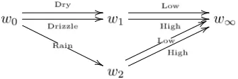
Example 1. Suppose that we would like to analyse the impact of weather on traffic in a medium-size city. For this purpose, take the explanatory variable “weather” with categories dry, drizzle, rain and a binary response variable “traf-fic” which represents the risk of traffic jam with categories low and high. Assume now that dry or drizzle have the same effect on traffic but that rain increases the risk of a traffic jam substantially. Figure 1 depicts a standard BN for this process. Note that without defing new random variables it is not possible to rep-resent the context-specific statement graphically (Dry weather and drizzle have the same impact on traffic).

Fig 1. BN of traffic example.

Here we propose a different graphical framework based on a tree to model longitudinal data, which are observed at not necessarily regular time-steps. We can incorporate many potential context-specific conditional independencies that may vary over time within this class. This enables us to estimate each model in a tractable and transparent way. In spite of their power and flexibility to model diverse domains, previous graphical models are not able to enjoy all these advantages.

Recently tree-based graphical models have been successfully used to describe various phenomena. This tree provides a flexible graphical support through which time sequences can be easily incorporated. Each path in the tree describes the various possible sequences of events a unit can experience. One such alter-native tree based model is the Chain Event Graph (CEG) (Smith and Anderson (2008); Freeman and Smith (2011a); Thwaites (2013); Barclay et al. (2014)). In a CEG not only conditional independencies, but also context-specific symme-tries, are directly depicted in the topology of the graph, see Example 1 below. Furthermore structural zero probabilities in the conditional probability tables are directly depicted by the absence of edges in its graph. See, for example, Smith and Anderson (2008); Barclay et al. (2013); Cowell and Smith (2014).

Example 1(continued). Observe that even without being formally familiar with the CEG semantic we can read from Figure2that the risk of traffic is identical for weather classed as dry or drizzle but differs in the case of rain.

Fig 2. CEG of traffic example.

It has been recently discovered that a CEG also retains most of the useful properties of a BN like closure to learning under complete sampling (Freeman and Smith (2011a)) and causal expressiveness (Thwaites (2013); Thwaites et al. (2010); Riccomagno and Smith (2009); Thwaites and Smith (2006a)). It also sup-ports efficient propagation of new information (Thwaites et al. (2008); Thwaites and Smith (2006b)). Hence CEGs provide an expressive framework for various tasks associated with graphical representation and statistical inference, espe-cially when the tree of the underlying sample space is asymmetric (French and Insua (2010)).

example Smith and Anderson (2008); Thwaites and Smith (2011) as well as many others). The topology of the CEG has hence been exploited to fully represent and generalize models such as context-specific BNs.

It has became increasingly apparent that in many contexts modelling variable changes explicitly over time provide better results. For a comparison between BNs and DBNs, see e.g. Rubio et al. (2014). Currently there is no such dynamic CEG defined in the literature. Freeman and Smith (2011b) developed one dy-namic extension of CEGs where the underlying probability tree is finite but the stage structure of the possible CEGs is allowed to change across discrete time-steps. This model, however, develops an entirely distinct class of models to the one considered here. It looks at different cohorts of units entering the tree at discrete time-points rather than assuming that repeated measurements are taken over time.

In this paper we develop the DCEG model class that extends the CEG model class so that it contains all dynamic BNs as a special case. In this sense we dis-cover an exactly parallel extension to the original CEG extension of the BN class. We show that any infinite tree can be rewritten as a DCEG, which repre-sents the originally elicited tree in a much more compact and easily interpretable form. A DCEG actually provides an evocative representation of its correspond-ing process. It allows us to define many useful DCEG model classes, such as the Repeating Time-Slice DCEG (RT-DCEG), that have a finite model parameter space.

A DCEG also supports conjugate Bayesian learning where the prior distribu-tion chosen in a family of probability distribudistribu-tionsAtogether with the available likelihood function yield a posterior distribution in the same familyA. This is a necessary requirement to guarantee analytical tractability and hence to design clever model search algorithms that are able to explore the large numbers of collections of hypotheses encoded within the DCEG model space. We further demonstrate that we can extend this framework by attaching holding time dis-tributions to the nodes in the graph, so that we can model processes observed at irregular time intervals. Our learning framework is closely related to the one developed by Nodelman et al. (2003) for CTBNs.

2. Background

In this section we revisit some graph notions that will be useful to discuss graphical models. Next we explain briefly the BN and DBN models and then define a CEG model. See Korb and Nicholson (2004); Neapolitan (2004); Cowell et al. (2007); Murphy (2012) for more detail on BNs and DBNs. The CEG concepts presented here are a natural extension of those in Smith and Anderson (2008); Thwaites et al. (2010); Freeman and Smith (2011a). These conceptual adaptations will allow us to directly use these concepts to define a DCEG model.

2.1. Graph Theory and conditional independence

Definition 1. Graph Let a graph G have vertex set V(G) and a (directed) edge setE(G), where for each edge e(vi, vj)∈E(G), there exists a directed edge

vi→vj,vi, vj ∈V(G). Call the vertex vi aparent ofvj if e(vi, vj)∈E(G)and let pa(vj)be the set of all parents of a vertex vj. Also, call vk a child of vi if

e(vi, vk)∈E(G)and let ch(vi)be the set of all children of a vertex vi. We say the graph is infinitewhen either the setV(G)or the set E(G)is infinite.

Definition 2. Directed Acyclic Graph

A directed acyclic graph (DAG) G = (V(G), E(G)) is a graph all of whose edges are directed with no directed cycles – i.e. if there is a directed path from ver-texvito vertexvj then a directed path from vertexvj to vertexvi does not exist.

Definition 3. Tree

A tree T = (V(T), E(T)) is a connected graph with no undirected cycles. Here we only consider a directed rooted tree. In this case, it has one vertex, called the root vertex v0, with no parents, while all other vertices have exactly

one parent. A leaf vertexinV(T)is a vertex with no children. Alevel Lis the set of vertices that are equally distant from the root vertex. A tree is an infinite tree if it has at least one infinite path.

Definition 4. Floret

Afloret is a subtreeF(si) = (V(F(si)), E(F(si))) of T,si ∈S(T)where:

• its vertex set V(F(si))consists of{si} ∪ch(si), and

• its edge set E(F(si)) consists of all the edges between si and its children in T.

There are various alternative ways of defining conditional independence. For the purposes of this paper it is more convenient to use the definition below.

Definition 5. Conditional Independence

A discrete random variableXa is conditionally independent of a discrete ran-dom variableXb given a set of discrete random variables X ={X1, . . . , Xn} if

for every triple(xa, xb,x_{), where}x_{= (x1, . . . , xn), we have that}

P(Xa=xa|Xb=xb,X =x_{) =P(Xa =xa|X =}x_{). (1)}

2.2. A Bayesian Network and a Dynamic Bayesian Network

A Bayesian Network is a probabilistic graphical model whose support graph is a DAG G= (V(G), E(G)). Each vertexvi∈V(G) represents a variableZi and the edge set E(G) denotes the collection of conditional dependencies that are assumed in the variable set. Here we assume that the vertex set V(G)) is well-ordered and that there can be a directed edgee(vi, vj) if and only ifi < j. Thus the variableZjis conditionally independent of variableZigiven the variable set

Zi

j ={Z1, . . . , Zj−1} \ {Zi} whenever an edgee(vi, vj) does not exist inE(G). Formally,

Zj ⊥⊥Zi|Zi

j ⇔e(vi, vj)∈/ E(G). (2) Recall that the concept of conditional independence plays a central role in this model class (Dawid (1998); Pearl (2009), Chapter 1, p. 1–40). Below we give a simple example that is more complex than the first since it entails not only context-specific independencies but also various asymmetric developments.

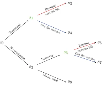
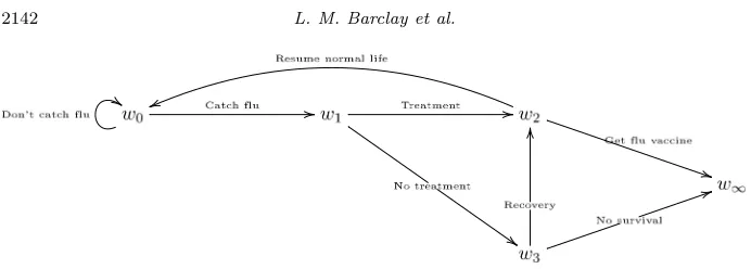
Example 2. An individual is at risk of catching flu. Having caught flu he either decides to take antiviral treatment or not (Treatment variable, see Figure 3). If he takes the antiviral treatment we assume that he will always recover. On the other hand if he does not take the antiviral treatment he either manages to re-cover or he dies from the virus (Rere-covery variable, see Figure 3). Given a full recovery the individual can either decide to go back to his normal life or to receive an influenza vaccine to prevent him from being at risk again (Vaccine variable, see Figure 3). We further hypothesise that the decision of taking a vaccine is conditionally independent of the decision to take the antiviral treatment given, of course, that the individual is alive. Thus the Recovery and Vaccine variables depends, respectively, on the Treatment and Recovery variables, but the Vac-cine variable is conditionally independent of the Treatment variable given the Recovery variable. Figure3shows a standard BN to model this process.

Fig 3. BN of flu example.

Another class of graphical model we will discuss and compare in this paper is the Dynamic Bayesian Network (DBN) which models the temporal changes in the relationships among variables. It extends directly the BN conception. A DBN G = (V(G), E(G)) can be interpreted as a collection of BNs {Gt = (V(Gt), E(Gt));t = 1,2, . . .} where the variables in time-slices t can also be affected by variables in the previous time-slices but not by variables in the next ones. These dependencies between time-slices are represented graphically by edges called temporal edges. Formally,V(G) =tV(Gt) andE(G) =

t[E(Gt)∪ Et], whereEt is the set of temporal edges{e(vi,τ, vj,τ);τ < t} associated with a BN Gt andvi,τ represents a variableZi in time-sliceτ < t.

2.3. A Chain Event Graph

A full description of this construction for finite processes can be found in Smith and Anderson (2008); Freeman and Smith (2011a); Thwaites et al. (2010). Here we summarise this development.

Definition 6. Event Tree

An event tree is a finite treeT = (V(T), E(T))where all vertices are chance nodes and the edges of the tree label the possible events that happen. A non-leaf vertex of a tree T is called a situation and S(T) ⊆ V(T) denotes the set of situations.

The path from the root vertex to a situationsi ∈S(T) therefore represents a sequence of possible unfolding events. The situation denotes the state that is reached via those transitions. Here we assume that each situation si ∈ S(T) has a finite number of edges, mi, emanating from it. A leaf node symbolises a possible final situation of an unfolding process. An edge can be identified by two situations si and sj (edge e(si, sj)) or by a situationsi and one of its corresponding unfolding eventsk (edgeesik).

Definition 7. Stage

We say two situations si andsk are in the same stage,u, if and only if

1. there exists an isomorphism Φik between the labels of E(F(si)) and

E(F(sk)), whereΦik(esij) =eskj, and

2. their corresponding conditional probabilities are identical.

When there is only a single situation in a stage, then we call this stage and its corresponding situation trivial.

If two situations are in the same stage then we assign the same color to their corresponding vertices. In other publications, for example Smith and Anderson (2008), corresponding edges of situations in the same stage are also given the same color. For clarity here we only color vertices and edges corresponding to non-trivial situations. We can hence partition the situations of the tree S(T) into stages, associated with a set of isomorphisms {Φik:si, sk∈S(T)}, and embellish the event tree with colors to obtain the staged tree.

Definition 8. Staged Tree

Astaged treeversion of T is one where

1. all non-trivial situations are assigned a color

2. situations in the same stage inT are assigned the same color, and 3. situations in different stages inT are assigned different colors.

We illustrate these concepts through a simple example on influenza, which we later develop further using a DCEG model.

Fig 4. Flu example.

treatment will not affect the individual’s probability to decide to get the vaccine. This demands that the probabilities on the edges emanating from s1, labeled

“resume normal life” and “get vaccine”, are identical to the probabilities on the edges emanating froms5with the same labels. This assumption can be visualized

by coloring the vertices of the event tree and their corresponding edges.

A finer partition of the vertices in a tree is given by the position partition. LetT(si) denote the full colored subtree with root vertexsi.

Definition 9. Position

Two situationssi, sk in the same stage, that is,si, sk∈u∈U,are also in the same position w if there is a graph isomorphism Ψik between the two colored subtreesT(si)→ T(sk). We denote the set of positions byW.

The definition hence requires that for two situations to be in the same position there must not only be a map between the edge sets E(T(si))→E(T(sk)) of the two colored subtrees but also the colors of any edges and vertices under this map must correspond. For example when all children of si, sk are leaf nodes then T(si) = F(si) and T(sk) = F(sk). Therefore si and sk will be in the same position if and only if they are in the same stage. But if two situations are further from a leaf, not only do they need to be in the same stage but also each child ofsi must correspond to a child ofsk and these must be in the same stage. This further applies to all children of each child ofsi and so on.

Definition 10. Chain Event Graph (Smith and Anderson (2008))

A CEG C = (V(C), E(C)) is a directed colored graph obtained from a staged tree by successive edge contraction operations. The situations in the staged tree are merged into the vertex set of positions and its leaf nodes are gathered into a single sink node w∞.

Fig 5. CEG of flu example.

Example 2 (continued). The hypothesis that recovering with or without treat-ment does not affect the probability of the individual taking the flu vaccine, placess1 ands5 in the same position. We then obtain the following CEG given

in Figure5with stages and positions given by:

w0=u0={s0}, w1=u1={s1, s5}, w2=u2={s2}, w∞={s3, s4, s6, s7, s8}

Note that the corresponding BN (Figure 3) cannot depict graphically the asymmetric unfolding of this process and the context-specific conditional state-ments.

3. Infinite probability trees and DCEGs

In this section we extend the standard terminology used for finite trees and CEGs to infinite trees and DCEGs. In the first subsection we derive the infinite staged tree, followed by a formal definition of the DCEG. The next subsection we extend the DCEG to not only describe the transitions between the vertices of the graph but also the time spent at each vertex. Finally we define a useful class of DCEG models.

3.1. Infinite staged trees

Clearly an infinite event tree can be uniquely characterized by its florets, which retain the indexing of the vertices ofT. The edges of each floret can be labeled as esij ∈E(F(si)), j= 1, . . . , mi, wheresihasmichildren. As noted above, we can

think of these edge labels as descriptions of the particular events or transitions that can occur after a unit reaches the root of the floret. In particular, we can also use the indexj = 1, . . . , mi to define a random variable taking values

{x1, . . . , xmi}associated with this floret.

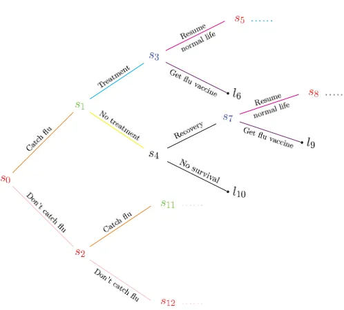
Fig 6. Flu example: the beginning of the infinite staged tree,T.

of the corresponding tree can be given (Figure 6), where implicit continuations of the tree are given by the notation ‘. . .’.

In our example the edgesE(F(s0))describe whether the individual catches the

flu(edgee(s0, s1))or not(edgee(s0, s2)), while the floret of vertexs1 describes,

having caught the flu, whether the individual takes the treatment(edgee(s1, s3))

or not (edge e(s1, s4)).

From the above example we can observe that each path within an infinite event tree is a sequence through time. To embellish this event tree into a proba-bility tree we need to elicit the conditional probaproba-bility vectors (CPVs) associated with each floretF(si). This is given by

πsi= (πsi1, πsi2, . . . , πsimi), (3)

whereπsij=P(esij|si) is the probability that the unit transitions fromsialong

thejth edge, and mi

j=1πsij = 1.

Collections of conditional independence (or Markovian) assumptions are in-trinsic to most graphical models. For an event tree these ideas can be captured by coloring the vertices and edges of the tree as discussed for CEGs in Sec-tion2.3. This idea immediately extends to this class of infinite trees.

a position. Observe that situations in the same position are always in the same stage but the inverse does not necessarily hold. This happens because stages impose probabilistic and topological equivalences for only one step ahead. In contrast position implies that these equivalences hold for the whole set of sub-sequent unfoldings along the event tree. Therefore if we have two distinct situ-ations in the same stage but in different positions, they will be represented by two different vertices with the same color.

Now call U the stage partition of T and define the conditional probability vector (CPV) on stageuto be

πu= (πu1, πu2, . . . , πumu), (4)

where u has mu emanating edges. If U is the trivial partition, such that ev-ery situation is in a different stage, then the coloring contains no additional information about the process that is not contained inT.

As above we can further define a CPV on each position:

πw= (πw1, πw2, . . . , πwmw). (5)

Surprisingly, the positions of an infinite tree T are sometimes associated with a coarser partition of its situations than a finite subtree of T with the same root. This is because in an infinite tree two situations lying on the same directed path from the root can be in the same position. This is impossible for two situations si, sk in a finite tree: the tree rooted at a vertex further up a path must necessarily have fewer vertices than the one closer to the root, so in particular no isomorphism betweenT(si) andT(sk) can exist. We give examples below which explicate this phenomenon.

Note that, we would normally plan to elicit the structural equivalences of the model – here the topology of the tree and stage structure associated with its coloring –beforewe elicit the associated conditional probability tables. This would then allow the early interrogation and adoption of the qualitative features of an elicited model before enhancing it with supporting probabilities. These structural relationships can be evocatively and formally represented through the graph of the CEG and DCEG. In particular this graph can be used to explore and critique the logical consequences of the elicited qualitative structure of the underlying process before the often time consuming task of quantifying the structure with specific probability tables.

Example 2 (continued). In the flu example we may have the staged tree as given in Figure6. Hence we assume that the probability of catching flu does not change over the months and does not depend on whether flu has been caught before. This implies that s0, s2,s5, s8 and s12 are in the same stage, as well

as all subsequent situations describing this event, which are not represented in Figure 6. Similarly, s1 and s11 are in the same stage, such that whether the

life after recovery is the same when he recovers after treatment as when he successfully recovers without treatment. This means that s3 and s7, as well as

all other situations representing the probability of returning to a normal life after recovery, are in the same stage. It can be seen from the staged tree that, in this example, whenever two situations are in the same stage, they are also in the same position as their subtrees have the same topology and the same coloring of their situations. Note that in this example the stage partition and the position partition of the situations coincides. Hence our stage and position partition is as follows:

w0=u0={s0, s2, s5, s8, s12. . .}, w1=u1={s1, s11, . . .},

w2=u2={s3, s7, . . .}, w3=u3={s4, . . .}. (6)

Not all paths in the tree are infinite and hence a set of leaf vertices,{l6, l9, l10, . . .},

exists.

3.2. Dynamic Chain Event Graphs

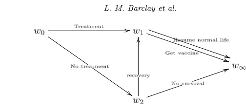
From the definition of a position, w, given a unit lies in w, any information about how that unit arrived at w is irrelevant for predictions about its future development. As for the CEG, the positions therefore become the vertices of the new graph, the DCEG, which we use as a framework to support inference. Further, colors represent probabilistic symmetries between positions in the same stage. Figure 7 depicts the DCEG corresponding to the staged tree shown in Figure6 above.

We can now define the DCEG, which depicts a staged tree (see Definition8

in Section 2.3) in a way analogous to the way the CEG represents structural equivalences.

Definition 11. Dynamic Chain Event Graph

ADynamic Chain Event Graph(DCEG)D= (V(D), E(D))of a staged tree

T is a directed colored graph with vertex setV(D) =W, the set of positions of the staged tree T, together with a single sink vertex, w∞, comprising the leaf nodes ofT, if these exist. The edge setE(D)is given as follows: Letv∈wbe a single representative vertex of the position w. Then there is an edge from wto a position w′ ∈W for each child v′ ∈ch(v), v′ ∈w′ in the tree T. When two positions are also in the same stage then they are colored in the same color as the corresponding vertices in the treeT.

We call the DCEGsimple if the staged treeT is such that the set of positions equals the number of stages,W =U, and it is then uncolored.

A DCEG is actually obtained from the staged tree by edge contraction op-erations. Observe also that if two situations are in the same positionwthere is a bijection between their corresponding florets. Thus we can take any vertex in wto represent it.

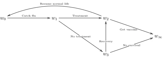
Fig 7. Flu Example: DCEG of the infinite staged tree.

actually a DCEG. However the CEG is always acyclic, whilst a DCEG can exhibit cycles – self-loops or loops across several vertices – when it has an infinite number of atoms but a finite graph. In this case a cycle represents a subprocess whose unfolding structure is unchangeable over time. We illustrate below that in many applications the number of positions of a staged tree is finite even though the tree’s vertex set is infinite. When this is the case the DCEG is a finite graph and therefore provides a succinct picture of the structural relationships in the process.

Example 2(continued). Figure7shows the corresponding DCEG of the staged tree given in Figure 6 with V(D) given in Equation 6. The loop from w0 into

itself illustrates that every month the individual could remain well and not catch flu. Alternatively, the individual may move to w1 at some point, meaning that

he has caught flu. In this case he can recover either by getting treatment (w1→ w2) or recover on his own (w1 → w3 → w2). Having recovered the individual

either decides to take a flu vaccine to avoid getting flu again (w2→w∞) or to simply resume his normal life and risk getting flu again (w2 → w0). Finally,

when not taking treatment, the individual may not recover, and hence move from

w3 to w∞. Here the position w∞ can be interpreted as representing stopped subprocesses whose two different stopping reasons are indicated by the labels (“Get flu vaccine” or “No survival”) of its incident edges.

3.3. DCEGs with holding time distributions

treatment, recovering, and receiving a vaccine are recorded and not the time until these events occur. These could, for example, be recorded retrospectively when measurements are taken a month later. Therefore, here the holding time distributions on a position without a loop into itself lose information.

However, in many cases our process is unlikely to be governed by regular time steps and it is much more natural to think of the time steps to be event driven. A process like this is naturally represented within a tree and hence a DCEG: when moving from one position to another the unit transitions away from a particular state into a different state associated with a new probability distribution of what will happen next. For example, the individual may not record whether he catches flu or not every month but instead monitor the time spent at w0 not catching flu, until one day he falls ill. Similarly, the time until seeing the doctor for treatment or the time until recovery may be of different lengths and so he spends different amounts of time at each position in the DCEG. Motivated by this irregularity of events, we look at processes in which a unit stays a particular time at one vertex of the infinite tree and then moves along an edge to another vertex. We hence define in this section a generalization of the DCEG, called the Extended DCEG, which attaches a conditional holding time distribution to each edge in the DCEG.

We call the time a unit stays in a situationsithe holding timeHsi associated

with this situation. We can further also define the conditional holding times associated with each edgeesij, j= 1, . . . , mi in the tree, denoted byHsij. This

describes the time a unit stays at a situation si given that he moves along the edge esij next. Analogously to this we can further define holding times on the

positions in the associated DCEG: We letHwbe the random variable describing the holding time on position w∈W in the DCEG andHwj, j= 1, . . . , mw the random variable describing the conditional time onwgiven the unit moves along the edgeewj next.

In this paper we assume that all DCEGs aretime-homogeneous. This means that the conditional holding time distributions for two situations are the same whenever they are in the same stage u. Hence, given the identity of the stage reached, the holding times are independent of the path taken. We denote the random variable of the conditional holding time associated with each stage by Huj, j = 1, . . . , mu. Time-homogeneity then implies that when two situations are in the same stageuthen their conditional holding time distributions are also the same. We note that a unit may spend a certain amount of time in position w∈ ubefore moving along the jth edge to a position w′ which is in the same stage. So a unit may make a transition into a different position but arrive at the same stage.

distribution may affect the transition probabilities and future holding times can provide an interesting extension to the DCEG and will be discussed in a later paper. Under these assumptions anExtended DCEG is defined below.

Definition 12. Extended DCEG

An Extended DCEG D = (V(D), E(D)) is a DCEG with no loops from a position into itself and with conditional holding time distributions conditioned on the current stage,u, and the next edge, euj, to be passed through:

Fuj(h) =P(Huj≤h|u, euj), h≥0,∀u∈U, j= 1, . . . mu. (7)

HenceFuj(h)describes the time a unit stays in any positionwmerged into stage

ubefore moving along the next edge ewj.

Consequently, given a positionw∈W(D) is reached, the joint probability of staying at this position for a time less than or equal tohand then moving along thejth edge is

P(Hwj ≤h, ewj|w) =P(Hwj≤h|w, ewj)P(ewj|w) =Fuj(h)πuj, w∈u. (8)

Finally, the joint density ofewj andhis

p(ewj, h|w) =πujfuj(h),

where fuj is the pdf or pmf of the holding time at stage u going along edge ewj, w∈unext.

An Extended DCEG with stage partitionU is hence fully specified by its set of conditional holding time distributions {Fuj(.) :u∈U} and its collection of CPVs {πu : u ∈ U}. Note that it is simple to embed holding times into the staged tree and into the DCEG. Example2 below discusses this issue in terms of qualitative and graphical modelling without using any specific holding time distribution. Observe also that an Extended DCEG differs from a DCEG in that the transition time between two positions depends on the initial and terminal stages. This fact links Extended DCEGs to semi-Markov processes.

Example 2(continued). Return again to the flu example from Section3.1with a slightly different infinite tree given in Figure 8. Instead of measuring every month whether the individual catches flu, the individual will spend a certain amount of time ats0 before moving along the tree. Hence the second edge

ema-nating froms0 in Figure 6and its entire subtree have been removed. As before,

it is assumed that the probability of catching flu and the decision to take treat-ment does not depend on whether the flu has been caught before. Also, recovery with or without treatment is assumed not to affect the probability of receiving a vaccine. The corresponding Extended DCEG is given in Figure9with positions given by

Fig 8. Variant of flu example: infinite treeT∗_.

Fig 9. Variant of the flu example: Extended DCEG of the infinite staged tree.

In comparison to Figure7the loop fromw0 into itself has been removed. Instead

the time spent at w0 is described by the holding time at position w0. Similarly,

the time until treatment is taken or not, the time until recovery or death and the time to receiving the flu vaccine or not are of interest and holding time distributions can be defined on these.

3.4. The repeating time-slice DCEG

Now we can define a useful DCEG class, called the repeating time-slice DCEG (RT-DCEG), whose graph is composed by two different time-slice finite sub-graphs.

Definition 13. Repeating Time-Slice DCEG

Consider a discrete-time process on I = {t0, t1, t2, . . .} characterised by a

Fig 10. Repeating Time-Slice DCEG.

to a variable Zp,t define the level Lp,t in the corresponding event tree. Denote

also by{spl,t0} and{spl,t1} the set of situations associated to the last variables

of time-slices t0 and t1, respectively. We have a Repeating Time-Slice DCEG

(RT-DCEG) when all previous conditions are valid and there is a surjection mapΥ :{spl,t0} → {spl,t1} such thatΥ(spl,t0) is in the same position asspl,t0

for allspl,t0.

The main characteristic of the RT-DCEG topology is that in the end of the second time slice the edges loop back to the end of the first time slice (see Figure10). Note that the levelsLp,t, t= 1,2, . . ., correspond to the same variable Zp. We will now illustrate a RT-DCEG modelling with a real-world example.

Example 3. We here consider a small subset of the Christchurch Health and Development Study, previously analysed in Fergusson et al. (1986); Barclay et al. (2013). This study followed around 1000 children and collected yearly informa-tion about their family history over the first five years of the children’s life. We here consider only the relationships of the following variables given below.

• Financial difficulty – a binary variable, describing whether the family is likely to have financial difficulties or not,

• Number of life events – a categorical variables distinguishing between 0,

1−2 and≥3 life events (e.g. moving house, husband changing job, death of a relative) that a family may experience in one year,

• Hospital admission – a binary variable, describing whether the child is admitted to hospital or not.

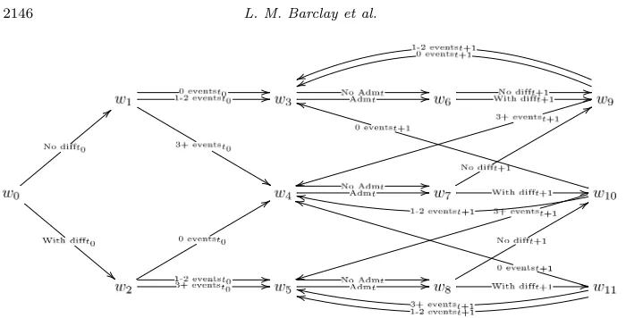
In this setting each time slice corresponds to a year of a child’s life start-ing from when the child is one year old, t0 = 1. A plausible RT-DCEG could

to w8. Also, observe that the variable describing the hospital admission is not

included at timet= 0, as it does not provide additional information under this assumption.

We start at w0 in order to follow the path an individual might take through

the DCEG across time. The first part of the graph describes the initial CPVs at time t0. It is first resolved whether or not the family has financial difficulties

(w0 → w1, w0 → w2) and whether the individual experiences 0,1−2 or ≥3

life events during this year (w1→w3,w1→w4,w2→w4,w2→w5). She then

reaches one of the three positionsw3,w4 and w5 describing a ‘health state’ the

individual is in before a hospital admission may occur. Independent of whether an admission has occurred or not (w6,w7,w8) she then moves to positions that

describe the same three health states. Then, given the individual is in one of the three health states (w3,w4,w5) at timet, fort≥t1, she traverses through the

graph in the following year according to the financial difficulty and number of life events in year t+ 1 and ends up in one of the three previous health states again.

Note that the positions of the RT-DCEG encode the entire history of a unit and we can trace back the full path a unit has taken through the graph. This is a property inherited from the event tree that supports the RT-DCEG graph. For instance, in Example 3 the probability of an individual having a hospital admission at time t is given by P(Adm= 1|wi) = πwi, i= 3,4,5. It therefore

depends on the position where the individual is located at timet. These positions are reached depending on the number of life events and the financial difficulty in that year and the health state of the previous year, which is again determined by the financial difficulty and the number of life events of the year before.

4. Bayesian learning of the parameters of an extended DCEG

In this section we present the learning process of a finite Extended DCEG which extends those for the CEG and is closely related to the learning framework for CTBNs proposed by Nodelman et al. (2003). Conjugate learning in CEGs is now well documented (Smith (2010); Freeman and Smith (2011a)), where the developed methods resemble also the ones used for discrete BN learning – see Korb and Nicholson (2004); Neapolitan (2004); Cowell et al. (2007); Heckerman (2008).

Here we consider only conditional holding time distributionsFujparametrised by a one-dimensional parameter λuj. Assuming random sampling and prior in-dependence of the vectorπ_{of all stage parameters and the vector}λ_{of different} holding time parameters, we can show that the posterior joint density ofπ _and λ_{is given by:}

p(π_,λ_|h,N,D) =p1(π|N,D)p2(λ|h,N,D), (9)

andp1(π|N,D) andp2(λ|h,N,D) are the posterior distributions of parameters π _andλ_{, respectively. See AppendixA for more details.}

Equation9makes sure that the parametersπ_andλ_{can be updated} indepen-dently. The Extended DCEG learning can then be divided in two distinct steps:

1. learning the stage parametersπ_{; and} 2. learning the holding time parametersλ_.

Learning the posteriorp1(π|N,D) therefore proceeds exactly analogously to learning within the standard CEG. Thus assuming local and global indepen-dence of stage parametersπ _{and random sampling – these conditions are also} assumed for conjugate learning of BNs – Freeman and Smith (2011a) show that with an appropriate characterisation each stage must have a Dirichlet distribu-tion a priori and a posteriori. Here we also assume these condidistribu-tions to update the stage parametersπ _{in a DCEG model. It then follows that}

π_{u∼Dir(αu1, . . . , αum}

u) (10)

and

π_u|N,D ∼Dir(αu1+Nu1, . . . , αumu+Numu), (11)

where αuj is the hyperparameter of the prior distribution associated with an edgej of stageuandNuj is the number of times an edgej of stageuis taken. As with all Bayesian learning some care needs to be taken in the setting of the hyperparameter valuesα_{u. In the simplest case we assume that the paths} taken on the associated infinite tree are a priori equally likely. We then specify the hyperparameters associated with each floret accordingly. Given that the Extended DCEG has an absorbing positionw∞ we can find, under the above

assumptions, theα_{u, u∈U of the Extended DCEG structureDderived from the} infinite tree by simply summing the hyperparameters of the situations merged. This direct analogue to Freeman and Smith (2011a) does not however work when no absorbing position exists, for then these sums diverge. Hence we need to take a slightly different approach. There are many possible solutions. Here we will adapt the concept of ‘equilibrium’ in Markov chains and thus make the simplest assumption that our prior beliefs with respect to the dynamic stages are ‘in equilibrium’ (see the discussion of Example 3 below. In other words, our prior beliefs are assumed to be the stationary distribution of the stage transition matrix that assigns the same probability to any path in the corresponding DCEG.

Note that when the holding time distributions are identical across the model space an Extended DCEG is indeed a DCEG and thus it is only necessary to learn the stage parametersπ_{. To compare two different models we can then use} the log Bayes Factor. We illustrate below how we can update the CPVs in a DCEG using the Christchurch example (Section3.4).

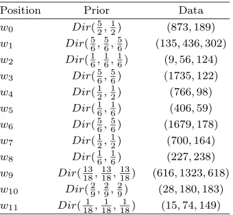
Table 1

Prior CPVs and data associated with each position

Position Prior Data

w0 Dir( 5 2,

1

2) (873,189)

w1 Dir( 5 6,

5 6,

5

6) (135,436,302)

w2 Dir(1 6,

1 6,

1

6) (9,56,124)

w3 Dir(5₆,5₆) (1735,122)

w4 Dir( 1 2,

1

2) (766,98)

w5 Dir( 1 6,

1

6) (406,59)

w6 Dir(5₆,5₆) (1679,178)

w7 Dir(1₂,1₂) (700,164)

w8 Dir( 1 6,

1

6) (227,238)

w9 Dir( 13 18,

13 18,

13

18) (616,1323,618)

w10 Dir(2₉,2₉,2₉) (28,180,183)

w11 Dir(₁₈1,₁₈1,₁₈1) (15,74,149)

of the Dirichlet distribution associated with each stage uas suggested above as follows: We first find the limiting distribution of the Markov process with state spaceW={w3, w4, w5, w6, w7, w8, w9, w10, w11} and with the following transition

probability matrix that assumes all paths in the graph are equally likely:

P = ⎛ ⎜ ⎜ ⎜ ⎜ ⎜ ⎜ ⎜ ⎜ ⎜ ⎜ ⎜ ⎜ ⎝

0 0 0 1 0 0 0 0 0 0 0 0 0 1 0 0 0 0 0 0 0 0 0 1 0 0 0 0 0 0 0 0 0 1 0 0 0 0 0 0 0 0 1₂ 1₂ 0 0 0 0 0 0 0 0 1₂ 1₂ 2

3 1

3 0 0 0 0 0 0 0

1 3

1 3

1

3 0 0 0 0 0 0

0 1₃ 2₃ 0 0 0 0 0 0

⎞ ⎟ ⎟ ⎟ ⎟ ⎟ ⎟ ⎟ ⎟ ⎟ ⎟ ⎟ ⎟ ⎠

So for example, the transition probability from position w9 is 2/3 to position w3, 1/3 to positionw4 and 0 to any other position. Solving the general balance

equations we then deduce that P(W =w3) =P(W =w6) = ₂₇5,P(W =w4) = P(W = w7) = 1₉, P(W = w5) = P(W = w8) = ₂₇1, P(W = w9) = 13₅₄, P(W = w10) = ₂₇2, P(W = w11) = ₅₄1. This limiting distribution together

with an equivalent sample size of 3 (equal to the largest number of categories a variable of the problem takes Neapolitan (2004)) determines the strength of the prior on each stage. Therefore the strength of stages in the same level has to sum up 3. Here this implies that we need to multiply the limiting distribution associated with each stage by 9 to obtain its corresponding strength. Further, assuming that the probabilities on the edges emanating from each position are uniform we can deduce the stage priors to be as given in Table 1.

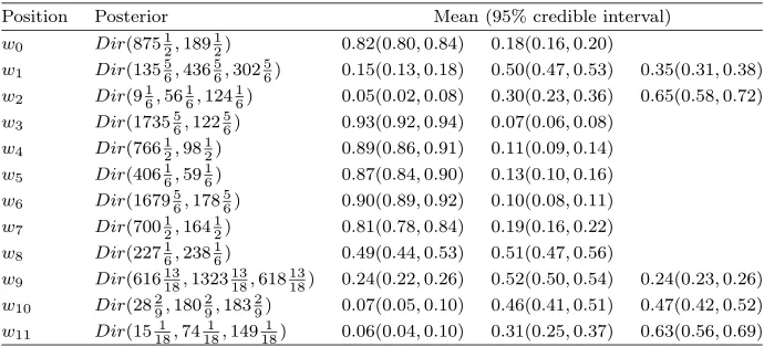
Table 2

Posterior CPVs and95%credible intervals

Position Posterior Mean (95% credible interval) w0 Dir(8751₂,1891₂) 0.82(0.80,0.84) 0.18(0.16,0.20)

w1 Dir(1355₆,4365₆,3025₆) 0.15(0.13,0.18) 0.50(0.47,0.53) 0.35(0.31,0.38)

w2 Dir(9 1 6,56

1 6,124

1

6) 0.05(0.02,0.08) 0.30(0.23,0.36) 0.65(0.58,0.72)

w3 Dir(1735 5 6,122

5

6) 0.93(0.92,0.94) 0.07(0.06,0.08)

w4 Dir(7661₂,981₂) 0.89(0.86,0.91) 0.11(0.09,0.14)

w5 Dir(406 1 6,59

1

6) 0.87(0.84,0.90) 0.13(0.10,0.16)

w6 Dir(1679 5 6,178

5

6) 0.90(0.89,0.92) 0.10(0.08,0.11)

w7 Dir(700 1 2,164

1

2) 0.81(0.78,0.84) 0.19(0.16,0.22)

w8 Dir(2271₆,2381₆) 0.49(0.44,0.53) 0.51(0.47,0.56)

w9 Dir(616 13 18,1323

13 18,618

13

18) 0.24(0.22,0.26) 0.52(0.50,0.54) 0.24(0.23,0.26)

w10 Dir(28 2 9,180

2 9,183

2

9) 0.07(0.05,0.10) 0.46(0.41,0.51) 0.47(0.42,0.52)

w11 Dir(15 1 18,74

1 18,149

1

18) 0.06(0.04,0.10) 0.31(0.25,0.37) 0.63(0.56,0.69)

year 2 to update the initial positions w0, w1 and w2 and then use the hospital

admissions variable of year 2, as well as years 3−5, to update the remaining CPVs. The data available for each position is presented in Table1.

Doing so we obtain the posterior distributions associated with each stage given in Table 2. We also present their corresponding means and 95% credible inter-vals. Observe that each stage has a Dirichlet posterior distribution whose param-eter is obtained by summing up the paramparam-eter of its Dirichlet prior distribution and corresponding sample vector.

Thus, for example, the expected probability of a child being admitted to hos-pital is 0.07 given she has reached position w3. This represents three possible

developments: i) she was previously in position w3 and had fewer than 3 life

events in the current year; ii) she was previously in state w4 and then had no

financial difficulties and less than 3 events in the current year; or iii) she was previously in state w4 and had financial difficulties but no life events in the

current year. Similarly, we have that the probabilities of an admission when reachingw4 andw5 are0.11and0.13, respectively.

stages. However using a Weibull distribution we are also able to allow for the possibility that the transition average rate varies over time by adjusting the hyperparameter κuj; for κuj <1 this rate decreases over time and forκuj >1 this rate increases over time. For more detail about the Weibull distribution and its use for Bayesian learning see Johnson et al. (1995).

To learn the parameters of the conditional holding time distributions, the priors onλuj are assumed to be mutually independent and have inverse-Gamma distributionsIG(αuj, βuj). This enables us to perform conjugate analyses which are analytically tractable. It also allows us to incorporate some background prior domain information. The hyperparameters αuj andβuj have a strict link with the expected mean and variance of the transitions events about which domain experts can provide prior knowledge. Of course in certain contexts the parameter independence assumption a priori may not be appropriate because the transition times are mutually correlated. In these situations it is likely that conjugacy would be lost, requiring other methods such as MCMC to find the corresponding posterior distribution.

Under the assumptions discussed above to obtain a conjugate learning, the posterior of the rate under this model is given by

λuj|huj, Nuj,D ∼IG(αuj+Nuj, βuj+ Nuj

l=1

(hujl)kuj_{), (12)}

wherehujl, l= 1, . . . , Nuj are the conditional holding times for each unitlthat emanates from a stageuthrough an edgej. Example 2 below exemplifies how we can apply this framework to learn the parameters of an Extended DCEG that has a loop and also a sink nodew∞.

Example 2 (continued). Recall again the Extended DCEG of the flu example given in Figure 9. To first set up the Dirichlet priors on π_{u and the}

Inverse-Gamma priors on λuj we again assume an uninformative prior on the paths of the associated tree. Since the equivalent sample size has to be greater than 2.5

to ensure that the prior Inverse-Gamma distributions have a mean, we chose an equivalent sample size of 3 to be only weakly informative. To determine the hy-perparametersα_{uof the Dirichlet priors we can here use the standard approach}

of summing the hyperparameters of the situations in each stage, as, due to the sink node w∞, the sum will not diverge as in the previous example.

Recall from Equation 9 that, for example, u1 ={s1, s10, s11, . . .}. Then

un-der the above assumptions and the tree structure in Figure 8 the situations in u1 have the distributions: v1 ∼Dir(1.5,1.5), v11 ∼ Dir(1.5ρ1,1.5ρ1), v12 ∼ Dir(1.5ρ2,1.5ρ2), where ρ1 = 0.25 and ρ2 = 0.125. Similarly, the next

situa-tions of u1 will have the distributions Dir(1.5ρ21,1.5ρ21),Dir(1.5ρ1ρ2,1.5ρ1ρ2), Dir(1.5ρ2ρ1,1.5ρ2ρ1),Dir(1.5ρ22,1.5ρ22), . . .. The infinite sum of the

hyperpa-rameters of these distributions is hence a geometric serie whose initial term is

3 and whose rate is equal to ρ1+ρ2 = 0.375. So we can obtain the

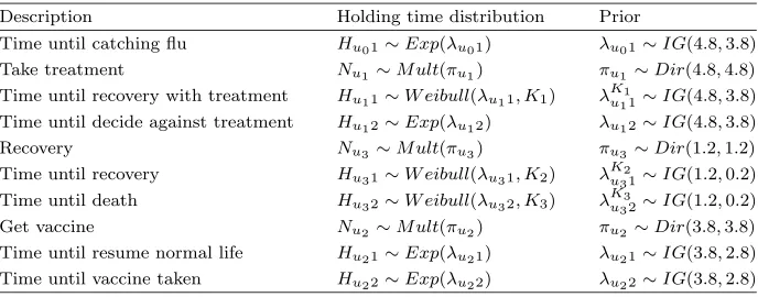
Table 3

Influenza Example: Prior distributions on CPVs and conditional holding times

Description Holding time distribution Prior

Time until catching flu Hu01∼Exp(λu01) λu01∼IG(4.8,3.8)

Take treatment Nu1 ∼M ult(πu1) πu1∼Dir(4.8,4.8)

Time until recovery with treatment Hu11∼W eibull(λu11, K1) λ

K1

u11∼IG(4.8,3.8)

Time until decide against treatment Hu12∼Exp(λu12) λu12∼IG(4.8,3.8)

Recovery Nu3 ∼M ult(πu3) πu3∼Dir(1.2,1.2)

Time until recovery Hu31∼W eibull(λu31, K2) λ

K2

u31∼IG(1.2,0.2)

Time until death Hu32∼W eibull(λu32, K3) λ

K3

u32∼IG(1.2,0.2)

Get vaccine Nu2 ∼M ult(πu2) πu2∼Dir(3.8,3.8)

Time until resume normal life Hu21∼Exp(λu21) λu21∼IG(3.8,2.8)

Time until vaccine taken Hu22∼Exp(λu22) λu22∼IG(3.8,2.8)

can be found in a similar way. They are given together with the priors of the conditional holding times in Table3.

In this example, it may further be plausible to assume an exponential distri-bution onHu01, which describes the time until catching flu, with scale parameter

λu01, the average time until the individual gets ill. Further it could be assumed

that Hu11 has the more general Weibull distribution, with scale parameterλu11

and with known shape parameterk1>1, describing the time until taking

treat-ment and recovering. As k1 >1 it is assumed that the recovery rate increases

with time. The time until the individual decides not to take the treatment could again be exponentially distributed with scale parameterλu12, i.e. it is assumed

to occur at a constant rate. Similarly to Hu11,Hu31 could also have a Weibull

distribution with known shape parameterk2>1. In contrast to this,Hu32could

have a Weibull distribution with scale parameterλu32and known shape

parame-terk3<1indicating that the death rate decreases with time. The holding times Hu21 andHu22 could again have exponential distributions with parametersλu21

and λu22 respectively. Here the time until getting the vaccine or resuming a

normal life is measured.

If Inverse-Gamma priors on λu01, λ

k1

u11, λu12, λu21, λu22, λ

k2

u31 and λ

k3

u32

are assumed, a conjugate analysis as described above can be carried out. The priors can be specified by assuming two conditions: i) a prior mean equal to

1 for all prior holding times; and ii) an equivalent sample size corresponding to the strength of the prior belief on the edge associated with each conditional holding time distribution (see Table3). Then, given a complete random sample of individuals going through the Extended DCEG for a certain length of time, the number of times, Nuj, each edge, euj, is used can be recorded, as well as the time spent at each position before moving along a particular edge. The prior distributions on π _andλ_{could then be updated in closed form by Equations12}

and11, respectively. The CPVs and expected time spent at each position, before moving along a certain edge, can thus be calculated.

an Extended DCEG structure given a complete random sampleL(D|h,N) sep-arates into two parts – one associated with the stages and another with the holding times:

L(D|h,N) =L1(D|N)L2(D|h,N). (13)

Then, the marginal likelihood of an Extended DCEG takes the form:

L1(D|N) =

u∈U

Γ(mu

j=1αuj) Γ(mu

j=1αu+Nu) mu

j=1

Γ(αuj+Nuj)

Γ(αuj) . (14)

After a little algebra the second component of the marginal likelihood associated with, for example, exponential holding times distributions can be written as:

L2(D|h,N) =

u∈U mu

j=1 βαuj

uj Γ(αuj)

Γ(αuj+Nuj) βuj+Nuj

l=1h αuj+Nuj

ujl

. (15)

When the prior distributions on λ _{are the same for all Extended DCEG} structures the log marginal likelihood, log L(D|h,N), can be written as a lin-ear function of scores associated with different components of the models. The overall linearity of the score is an important property to be explored to devise clever techniques for traversing the Extended DCEG model space since the size of this space is vast without further constraints.

5. Discussion

In this section we discuss the association between DCEGs and three other dy-namic models: DBNs, Markov chains and semi-Markov processes.

5.1. The relationship between a DBN and a DCEG

Here we demonstrate that discrete DBNs (see Section2.2) constitute a special DCEG class. We then discuss some pros and cons in using one or other model. Smith and Anderson (2008) and Barclay et al. (2013) have shown how a BN can be written as a staged tree and hence as a CEG. This can be simply extended to a dynamic setting and we explain below how a DBN can be represented as an infinite staged tree and therefore as a DCEG. It is also easy to check that many other processes such as dynamic context-specific BNs (Boutilier et al. (1996); Friedman and Goldszmidt (1998)) or dynamic Bayesian multinets (Geiger and Heckerman (1996); Bilmes (2000)) are amenable to this representation. Here to match our methods against the usual formulation of the DBN we are focusing only on the DCEG (Section 3.2), where one-step transitions are known and holding times do not need to be explicitly considered.

number of values. The variablesZtthen form a time-slice of the DBN for each time pointt. In the most general case, the DBN onZthas an associated infinite acyclic directed graphG where the componentZp,t ofZthas parents

pa(Zp,t) ={Zq,s:s < t, q∈ {1, . . . , ns}} ∪ {Zq,s:s=t, q∈ {1, . . . , p−1}}.

Next we claim that any general DBN can be written as an infinite staged tree. To demonstrate this, we first show how to write the variables of the DBN as an infinite tree. We then define the conditional independence statements of the DBN by coloring the florets in the tree to form a stage partition of the situations.

Reindex the variables as Zk =Zp,t, k = 1,2,3, . . . so that, whenever Zi = Zq,s ∈ pa(Zp,t), then the index i < k. This will ensure that parent variables come before children variables and time-slices come before each other. There is clearly always such an indexing because of the acyclicity and time element ofG. This gives a potential total ordering of the variables in{Zt:t∈I}from which we choose one. Leta(Zk) ={Zi:i < k} be the set of antecedents ofZk for the chosen variable order. Note thatpa(Zk,t)⊆a(Zk).

By the assumptions of the ordering the components up to index k can be represented by a finite event tree denoted by Tk = (Vk, Ek). Recall from Sec-tion3.1that each floret in the tree can be associated with a random variableZi and the edgeseij, j= 1, . . . , mi describe themi values in the sample space that this random variable can take. Hence the paths in the treeTk correspond to the set of all combinations of values that variablesZk can take. Then a sequential construction of the stochastic process allows us to define a set of trees{Tk}_k≥1, such thatTk is a subtree ofTk+1, recursively as follows:

Let Lk = Vk \Vk−1 be the set of leaf vertices of Tk. Let also lki ∈ Lk, i= 1,2, . . . , Nk be a single leaf vertex iofTk which has Nk leaf vertices.

1. Fork= 1, letT1 be the floret, F(s0), associated withZ1 which can take m1 values. Therefore V1 = {s0, l11, l12, . . . , l1m1} and E1 = {es0j : j =

1, . . . , m1}. Given Tk = (Vk, Ek), define the edge set of the tree Tk+1 as follows:

Ek+1=Ek∪Ek++1,

where

E_k+₊₁={elkij:lki∈Lk, j= 1,2, . . . , mk+1} (16)

is a set of Nk×mk+1 new edges such asmk+1 edges emanate from each vertex lki, i = 1,2, . . . , Nk. Each of these edge elkij describes a specific

value that the random variableZk+1can take. To define the vertex set of

Tk+1, attach now a new leaf vertex to each of the edges inEk++1 and let

Vk++1={ch(lki) :lki∈Lk} (17)

Fig 11. A simple DBN for Christchurch Example.

2. The infinite tree T of this DBN is now simply defined as T = (V, E), where the vertex and edges sets are, respectively, given by

V = lim

k→∞Vk and E= limk→∞Ek.

Note that the infinite length directed paths starting from the root of this tree correspond to the atoms of the sample space of the process.

We demonstrate this recursive construction of the infinite tree below.

Example 4. Here we remodel the Christchurch example (Section 3.4) where we take only the binary variables Financial Difficulty and Hospital Admission into account. Let Z1,t andZ2,t denote, respectively, the variables Financial

Dif-ficulty and Hospital Admission in time-slice t. Suppose now that the financial life enjoyed by a family in timetdepends only on its previous financial situation in time t−1. Assume also that the probability of a child been admitted in the hospital in time t depends if she visited the hospital in timet−1 as well as on the current financial difficulty faced by her family. The DBN given in Figure 11

represents this process over time. Note that this is a 1-Markov BN: a variable is only affected by variables of the previous and current time-slices.

We can now reindex the variables of the DBN as follows:

Z1=Z1,t0,Z2=Z2,t0,Z3=Z1,t1,Z4=Z2,t1,Z5=Z1,t2,Z6=Z2,t2, . . .

where Zi represents a variable Financial Difficulty, if the index i is an odd number, and a variable Hospital Admission, otherwise. Thus for example in the event tree a(Z6) = {Z1, Z2, Z3, Z4, Z5} will be the antecedents of the variable

hospital admission associated with the third time-slice (Z2,t2).

Because we have definedZ1=Z1,t0,T1hence corresponds to the tree given in

Figure12 (a) with root vertexs0 and two emanating edges labeled No difficulty

and With difficulty. To obtainT2 (Figure12 (b)) fromT1 attachm2= 2edges

to each leaf vertex ofT1as defined by Equation16and attach a child to each new

edge as defined in Equation 17. Similarly, to obtainT3 fromT2 attachm3 = 2

edges describing Z3 = 0 and Z3 = 1 to each leaf of T2 and attach a new leaf

to each new edge. Continuing in this way a representation of the infinite tree is provided in Figure 17(Appendix B), where again the notation ‘. . .’ describes the continuation of the process.

Fig 12. Illustration ofT1 andT2 of a DBN.

Section 3.1. The resulting staged tree then encodes the same conditional inde-pendencies as the DBN.

Notice that the vertex lki ∈ Vk ⊆V labels the conditioning history of the variableZk+1 based on the values of its antecedent variables. By the definition of a DBN

Zk+1⊥⊥a(Zk+1)|pa(Zk+1), (18)

which means that a variable Zk+1 is independent of its antecedents given its parents. So by the DCEG definition the leaf nodeslki1 andlki2 associated with

the event treeTk are in the same stage whenever their edge probabilities are the same. More formally

P(elki1j|lki1) =P(elki2j|lki2) (19)

for all edgeselki1j andelki2j, j= 1, . . . , mk+1 or alternatively,

P(Zk+1=zk+1|lki1) =P(Zk+1=zk+1|lki2), (20)

wherezk+1 is a value the variableZk+1 can take. If this is true then we assign the same color tolki1 as tolki2. Thus the corresponding DCEG follows directly

from the staged tree by performing edge contraction operations according to the position partition (see Section3.2).

Example 4(continued). Recall the previous Example 4. Assume now that the conditional probability tables remain the same across the time-slices t, t ≥t1,

Fig 13. Illustration of the RT-DCEG of a DBN.

t, t ≥ t1, only changes – in this case positively – if a family currently enjoys

a good financial situation and their child was not admitted to the hospital in the previous time-slice. This probability is hypothesised to be equal to the one assigned to a child that lives in a financially stable family in the first time-slice. Appendix Bshows the staged tree corresponding to these hypotheses. Note that the colors alternate between odd and even levels because of the invariance of the conditional probability tables over time. Observe that it is not possible to represent these context-specific conditional statements graphically using a DBN model on these variables although they are encoded in the DBN’s conditional probabilistic tables. In contrast, these additional conditions are not only directly depicted in a DCEG – which is actually a RT-DCEG – but also the corresponding graph is quite compact and easily interpreted (Figure 13).

the corresponding DCEG. But when, as is often the case, many combinations of values of states are logically impossible and the number of non-zero probability transitions between states is small then the DCEG depicts these zeros explicitly and can sometimes be topologically simpler than the DBN.

Consider the staged tree of Example4(Figure17, AppendixB). If the condi-tional probability tables of the BN state thatP(Z2,t0 = Adm|Z1,t0= No diff) =

0 then the edge describing this probability can be omitted from the tree and the tree is hence reduced to three quarters of its size. Hence unlike the BN and its dynamic analogue, as well as depicting independence relationships the DCEG also allow us to read zeros in the corresponding transition matrix, represented by missing edges in the tree. This is particularly helpful when representing pro-cesses which have many logical constraints. However, these gains imply that the DCEG model space scales up super-exponentially with the number of variables. Here the main challenge is to devise clever algorithms to search the DCEG model space.

5.2. DCEG and Markov chain

In this section we use some examples to illustrate some topological links between DCEG graphs and state-transition diagrams of Markov Chains. These connec-tions constitute a promising start pointing to extend many of the well-developed results on Markov processes to the DCEG domain – see, for example, the use of limiting distribution to initialise the DCEG learning process (Section4). In its turn, the DCEG framework can be used to verify if there is statistical evidence that supports modelling a real-world process as a Markov Chain, and (if there is) to infer its corresponding transition matrix.

Note that the topology of the DCEG graph resembles the familiar state-transition diagram of a Markov process, where the positions of the DCEG can be reinterpreted as states of the Markov process. However, as mentioned at the end of Section 3.1 the DCEG is usually constructed from a description of a process as a staged tree rather than from a prespecified Markov chain. Thus there are also some differences between the DCEG graph and standard state-transition diagrams such as the one-to-one relationship between the atoms of the space of the DCEG and its paths and its coloring as will be illustrated in the simple examples below.

Example 5. Example of a Markov Chain I

Let{Xn :n∈N_{}be a discrete-time Markov process on the state space{a, b, c}} with transition matrix P given by

P=

⎛

⎝

0.2 0.3 0.5 0.5 0.3 0.2 0.5 0.3 0.2

⎞

⎠,

Fig 14. State-transition diagram of the Markov process in Example5.

However, the DCEG representation gives a different structure, which becomes apparent when looking first at the tree representation of the problem. As the process is infinite, the number of situations of the tree is also infinite. The initial situations0, the root of the tree, has emanating edges which represent the choice

of initial state with associated CPV πs0 = (0.4,0.4,0.2). The other situations

could be indexed as{si,n, i=a, b, c, n∈N_{}with CPVsπs}

a,n= (0.2,0.3,0.5)and

πsb,n=πsc,n= (0.5,0.3,0.2). It is then immediate that the corresponding DCEG

only has three stages and positions with the stage and position partition given by

u0=w0={s0}, u1=w1={sa,n, n∈N}, u2=w2={sb,n, sc,n, n∈N}.

There is no w∞ as all paths are infinite and hence no leaf vertices exist in the tree. The DCEG can then be drawn as given in Figure 15a and the associated CPVs are πw0 = (0.4,0.4,0.2), πw1 = (0.2,0.3,0.5) and πw2 = (0.5,0.3,0.2).

For a better comparison the CPVs have here also been attached to the edges of the DCEG. Figure15b depicts the same process when it has a degenerate initial distributionπs0 = (1,0,0).

Even here, where the process is initially defined through a transition matrix, the graph of the DCEG automatically identifies states which have equivalent roles: here state b being identified with state c, and illustrates the identical

conditional probabilities associated with the two states by puttingsb,nandsc,n, forn∈N_{in the same positionw1 in Figure15.}

The DCEG also depicts explicitly the initial distribution of the process given by the edges emanating fromw0and acknowledges the initially elicited distinc-tions of the statesbandcthrough the double edge fromw0tow2. Observe also that if a process has a degenerate initial distribution – for example, the one depicted in Figure15b – the DCEG will show this phenomenon transparently and it only implies minor changes in the DCEG topology.

These topological properties often have important interpretive value, as the DCEG can discover a different partition of the states of a variable or even help to construct new informative variables to represent a problem. Further, any residual coloring, inherited from the staged tree allows us to elaborate the structure of the transitions in a natural and consistent way, highlighting some possible common underlying structures between the states of a Markov process. This can bring new questions and motivate a deeper understanding of the pro-cess under analysis. For example, the state-transition diagram and DCEG graph (Figure16) corresponding to the simple Example6 are identical except for the colors. By coloring the positions red, the DCEG model stresses that their tran-sition processes are probabilistically identified with each other (i.e. they are in the same stage). In real-world problems if these coloring properties appear in the best scoring model based on the given data set, then these features are ex-plicitly depicted and fed back to domain experts who can then speculate about the possible reasons for their presence.

Example 6. Example of a Markov Chain II

A coin is tossed independently, with probabilityP(H) =λof throwing heads and probability P(T) = 1−λ = ¯λ of throwing tails. The coin is tossed until

N heads have appeared when the game terminates. Its DCEG has thus N+1

positions describing whether0,1,2,. . .,N−1 orN heads have been tossed and is given in Figure16.

Notice here that because each toss has the same probabilityλof heads the posi-tionsw0, w1, w2, . . . , wN−1are all in the same stage and so its verticesw0, w1, w2, . . . , wN−1 are colored red. If this was a model discovered from observations an

expert could immediately deduce that a coin with the same probability of heads was being used at each time.

Being able to embed the state-transition diagrams and to register the entire unfolding process in its coloring and topology, a DCEG model provides a very expressive graphical representation of a stochastic process. After searching a well-fitting DCEG model and learning it, we would then be able to identify

if there is at least a subgraph in this DCEG model that represents a Markov process. If this is possible, this will enable us to further explore some asymptotic behaviours of this subprocess using the well-established Markov theory.

5.3. Extended DCEG and semi-Markov process

As there is a connection between a DCEG and Markov processes, an Extended DCEG is closely linked to semi-Markov processes (Barbu and Limnios (2008); Medhi (1994)). These are a generalization of Markov processes that allow for the holding times to have any distribution instead of restricting them to have a geometric distribution (discrete-time Markov processes) or an exponential distribution (continuous-time Markov processes). We recall the definition of a semi-Markov process below:

Definition 14. Semi-Markov Process (Medhi (1994))

Let {Yt, t ≥ 0} be a stochastic process with discrete state space and with transitions occurring at times t0, t1, t2, . . .. Also, let {Xn, n ∈ N} describe the

state of the process at time tn and let Hn be the holding time before transition toXn. HenceYt=Xn on tn≤t < tn+1. If

P(Xn+1=j, Hn+1≤t|X0, X1, . . . , Xn, H1, . . . , Hn)

=P(Xn+1=j, Hn+1≤t|Xn), (21)

then {Xn, Hn} is called a Markov Renewal process and {Yt, t ≥ 0} a semi-Markov process. Also,{Xn, n∈N_{}is the embedded Markov chain with transition} probability matrixP = (pij), wherepij =P(Xn+1=j|Xn =i).

A semi-Markov process is usually specified by an initial distribution α and by its semi-Markov kernelQwhoseijth _{entry is given by}

Qij(t) =P(Xn+1=j, Hn+1≤t|Xn=i). (22)

We assume here that all Markov processes considered are time-homogeneous and hence the above equations do not depend on the indexn. In order to illustrate a link between the Extended DCEG and semi-Markov processes we write the semi-Markov kernel as

Qij(t) =pijFij(t), (23)

where

Fij(t) =P(Hn+1≤t|Xn+1=j, Xn=i) (24)

is the conditional holding time distribution, i.e. the holding time at Xn = i assuming that we move to Xn+1=j next andpij is given in Definition14. We can then show that a particular subclass of the time-homogeneous Extended DCEG corresponds to a semi-Markov Process.