White Rose Research Online URL for this paper:
http://eprints.whiterose.ac.uk/107943/
Version: Accepted Version
Article:
Joshi, Chaitanya, Larson, Jonas and Spiller, Timothy P. orcid.org/0000-0003-1083-2604
(2016) Quantum state engineering in hybrid open quantum systems. Physical Review A.
043818. ISSN 1094-1622
https://doi.org/10.1103/PhysRevA.93.043818
[email protected] https://eprints.whiterose.ac.uk/ Reuse
Items deposited in White Rose Research Online are protected by copyright, with all rights reserved unless indicated otherwise. They may be downloaded and/or printed for private study, or other acts as permitted by national copyright laws. The publisher or other rights holders may allow further reproduction and re-use of the full text version. This is indicated by the licence information on the White Rose Research Online record for the item.
Takedown
If you consider content in White Rose Research Online to be in breach of UK law, please notify us by
Chaitanya Joshi,1,∗ Jonas Larson,2 and Timothy P. Spiller1
1
Department of Physics and York Centre for Quantum Technologies, University of York, Heslington, York, YO10 5DD, UK
2
Department of Physics, Stockholm University, Albanova physics center, Se-106 91 Stockholm, Sweden (Dated: March 30, 2016)
We investigate a possibility to generate non-classical states in light-matter coupled noisy quan-tum systems, namely the anisotropic Rabi and Dicke models. In these hybrid quanquan-tum systems a competing influence of coherent internal dynamics and environment induced dissipation drives the system into non-equilibrium steady states (NESSs). Explicitly, for the anisotropic Rabi model the steady state is given by an incoherent mixture of two states of opposite parities, but as each parity state displays light-matter entanglement we also find that the full state is entangled. Furthermore, as a natural extension of the anisotropic Rabi model to an infinite spin subsystem, we next explored the NESS of the anisotropic Dicke model. The NESS of this linearized Dicke model is also an in-separable state of light and matter. With an aim to enrich the dynamics beyond the sustainable entanglement found for the NESS of these hybrid quantum systems, we also propose to combine an all-optical feedback strategy for quantum state protection and for establishing quantum control in these systems. Our present work further elucidates the relevance of such hybrid open quantum systems for potential applications in quantum architectures.
PACS numbers: 42.50.Pq, 42.50.Ct, 03.67.Bg, 03.65.Yz
I. INTRODUCTION
Light-matter coupled quantum systems are now seen as novel composite systems for the exploration of vari-ous tasks in quantum computation and information pro-cessing, as well as for testing foundations of quantum physics [1–3]. These hybrid systems promise to com-bine disparate quantum degrees of freedom in construct-ing scalable quantum architectures [1, 4]. In particular, the idea is to take ‘the best of two worlds’: matter pro-vides good candidates for storage of quantum informa-tion, while light (photons) are superior when it comes to transmitting or sending quantum information, with interactions between these provide processing. For ex-ample, photons can be sent between different parties in order to create entanglement over macroscopic distances. However, physical quantum systems, in this case espe-cially the light part, invariably also couple to their ex-ternal environments [5, 6]. It is commonly argued that non-classical states, including entangled states, are ex-tremely sensitive to noise and dissipation. For exam-ple, environment induced decoherence tends to reduce quantum-coherent superpositions to incoherent mixtures [7]. Quantum state engineering strategies have therefore taken a center stage in salvaging quantum coherence in hybrid quantum systems [1, 8]. It is clear that for using photons as information carriers between different mat-ter subsystems, sustainable entanglement between light and matter is a necessity, i.e. such quantum correlations should survive any realistic decoherence/noise affecting the photons.
∗Electronic address: [email protected]
In a somewhat parallel approach, noisy coupled quan-tum systems have been proposed as exciting avenues for controlled generation of multi-partite entangled states [9]. The interplay between coherent and incoherent dy-namics in interacting multi-partite open quantum sys-tems can result in the generation of steady states which exhibit exotic quantum character [10, 11]. To take a par-ticular example relevant for this work, for open optical systems the dynamics can often be well described by a Lindblad type master equation
˙ˆ
ρ=−i[ ˆHS,ρˆ] +γLˆAˆρ,ˆ (1)
where ˆρ is the system’s state, ˆHS the system
Hamilto-nian, and ˆLAˆρˆ is the Lindblad super operator
render-ing the effects of the reservoir on the system ( ˆA is the so called quantum jump operator, and we note that ˆHS
may be modified from the closed system Hamiltonian due to the interaction with the environment). The steady state is solved by lettingi[ ˆHS,ρˆss]−γLˆAˆρˆss = 0. It
fol-lows that if ˆρss is a dark state, i.e. LˆAˆρˆss = 0, then
ˆ
ρss must also commute with ˆHS, e.g. being an
eigen-state of the Hamiltonian. However, this is not the only possibility for having a steady state; both contributions might be non-zero but also exactly cancel each other. This would mean that the unitary evolution ‘balances’ the non-unitary evolution. For infinite systems, this in-terplay may result in non-equilibrium phase transitions between phases supported either by the first or the sec-ond term in Eq.(1) [10, 11]. That is to say that ˆρss
changes qualitatively and shows non-analytic properties at some critical γc. For finite systems, on the other
hand, such a transition is smooth/analytic, but never-theless for the intermediate stages between the two ex-tremes non-classical states may persist. In this work
we explore this scenario and examine the possibility of generating non-classical states in two open quantum sys-tems that have served as work horses in quantum optics for more than half a century, namely the Rabi [12] (or non-Rotating-Wave-Approximation (non-RWA) Jaynes-Cummings model [13]) and the Dicke model [14]. In a way, in our study these two models are at the two ex-tremes of the quantum spectrum; the Rabi model which couples a single spin-1/2 particle to a boson or photon mode lives in the deep quantum regime, while what we term the Dicke model considers instead a particle with an infinite large spinS (almost classical) coupled to the boson mode. As already mentioned, the main source of decoherence is very often photon absorption and we thereby consider a Lindblad term with ˆA= ˆabeing the photon annihilation operator. This photon loss mecha-nism aims at emptying the boson mode (the only dark state is the vacuum). However, for a large light-matter coupling in the Hamiltonian even the ground state (in the absence of environmental coupling) becomes a ‘highly excited’ (from the perspective of photon number) state, and so the two dynamical contributions in the evolution of the hybrid system must be balanced in order to sup-port a NESS. We will demonstrate that as a result of this competition between unitary and non-unitary evolution, for both models a NESS exists that possess non-classical features in terms of light-matter entanglement. Further-more, especially for the Rabi model this NESS reflects the well known parity symmetry of the original Hamil-tonian; the NESS consists of an incoherent mixture of different parity states.
In the second half of the paper we explore possibilities to systematically enrich and enhance the non-classical properties of the NESS. More precisely, although envi-ronment induced dissipation potentially can be tailored to achieve desired quantum states [15], establishing quan-tum control over various dissipation channels is also an important benchmark toward realizing a useful quantum architecture [16]. Thus, it is desirable to construct quan-tum control schemes for hybrid quanquan-tum processors if, for instance, one is interested in initial quantum state preser-vation [17]. Along these lines we will use an all-optical coherent feedback strategy [18–20] to achieve quantum state preservation. It is important to appreciate that such a scheme is different from just tailoring the dissipa-tion channels as it involves active feedback to the system. As outlined in Refs. [18, 19], under the assumption that the time-delay introduced by the feedback loop is negli-gible it is indeed possible to establish a complete control over the dissipative dynamics. Going beyond such ideal-ized sudden feedback control, we will conclude by briefly commenting on the prospects of our scheme by combin-ing it with a time-delayed feedback control scheme as previously studied both in the classical [21] and quan-tum domains [22, 23].
The paper is organized as follows. In Sec.II we intro-duce our first physical model describing the interaction between a quantized bosonic mode and a single two-level
system. We explore the general structure of the NESS ˆρss
(being of an interesting form) and extract the sustainable entanglement between the two subsystems. The follow-ing Sec.III addresses the question whether non-classical features survive in the ‘classical limit’ in which the two-level system is turned into an infinite onei.e. identifying the linearized Dicke model. And indeed, entanglement is sustained also in this case. Having discussed these two model examples, in Sec. IV we combine a coherent all-optical feedback scheme for quantum state protection in open quantum systems. While entanglement is sustain-able in the original open systems, the feedback scheme allows for increasing the desired properties. Finally, we conclude the paper with a short discussion in Sec. V.
II. MODEL A - ANISOTROPIC RABI MODEL
The quantum Rabi model describes the interaction be-tween a quantized bosonic field and the simplest quan-tum mechanical model, a single two-level system or qubit [12]. Despite its simplicity, the quantum Rabi model had eluded an exact solution for many decades and it was only recently that an analytical solution was obtained [24], with continuing debate as to the completeness of this so-lution and the existence of other possible soso-lutions [25]. Nonetheless, over the years the quantum Rabi model has turned out to be an ubiquitous physical model and has found applications in understanding a wide variety of physical systems, including trapped ions, superconduct-ing qubits, optical and microwave cavity QED, circuit QED, among others [26]. In some cases the two-level system may be an exact description of the matter part of the hybrid system (when it is indeed a spin-1/2 par-ticle), but in many cases the two-level description is an approximation of a more complicated matter sub-system. In its most simplified form the quantum Rabi model takes the form (with~=1 and neglecting the vacuum
en-ergy of the boson mode)
ˆ
HRM=ωˆa†ˆa+Ω
2ˆσz+λ(ˆa
†+ ˆa)(ˆσ++ ˆσ−). (2)
Here, ˆaand ˆa†are the annihilation and creation operators
for the bosonic field of frequencyω, ˆσ± = (ˆσx±iˆσy)/2
with ˆσx,y,z the Pauli matrices for the two-level system, Ω
is the energy level splitting between the two levels, and the coupling strength between the bosonic mode and the two-level system is represented as λ (≥ 0). Through-out we will use dimensionless parameters such that we scale all frequencies by ω and time by ω−1.
Neverthe-less, we keepω in all expressions in order to keep track of all terms and instead always useω = 1 in any calcu-lations. The counter-rotating terms in the Hamiltonian (2), ˆa†σˆ+ and ˆσ−ˆa, do not conserve the excitation
the RWA results in the widely studied Jaynes-Cummings model which can be straightforwardly solved [13, 30]. As evident through several standard cavity-QED exper-iments, the atom-field coupling λ is normally orders of magnitude smaller than the bare transition frequencies
ω,Ω, and this makes the RWA a valid approximation to simplify the quantum Rabi model [3]. The straight-forward solvable nature of the Jaynes-Cummings model results from the presence of a continuous U(1) symme-try; the total number of excitations ˆN = ˆa†ˆa+ 1
2σˆz is
preserved. This should be contrasted with the discrete
Z2 parity symmetry of the Rabi model characterized by
the unitary ˆUZ2 = exp
i ˆa†aˆ+ ˆσ+ˆσ−
π
. The action of ˆUZ2 is to flip the signs of ˆa, ˆa
†, ˆσ
x,y while leaving ˆσz
invariant. Thus, the Rabi model has a lower symmetry than the Jaynes-Cummings model, which naturally is the reason why finding an exact Rabi solution is very hard.
The RWA simplified quantum Rabi model is undoubt-edly one of the most celebrated models in quantum optics and has received well deserved attention [30–32]. How-ever, there has been a recent surge of interest in exploring hybrid quantum systems in the so-called “ultra-strong” coupling regime [33]. In this ultra-strong coupling regime the atom-field coupling strength λcan approach a non-negligible fraction of the bare transition frequenciesω,Ω, thereby making the Jaynes-Cummings model a non-valid approximation for the quantum Rabi model [34]. From the discussion of the introduction, it should be clear that in order to generate large steady state entanglement the coupling λ should be made as large as possible (al-lowed by other approximations like the two-level approx-imation). As λ > √ωΩ the ground state of the Rabi model undergoes a qualitative change [32, 35] where the field builds up a large non-zero photon number. In the Dicke model this marks the normal-superradiant phase transition [36]. This extremely large λregime has been termed the “deep strong” coupling regime [37]. Thus, as the ultra-strong coupling regime has recently been realized in certain (non-driven) circuit QED architec-tures [33] (λ∼ω/10), we would like to explore the quan-tum Rabi model further, into the deep strong coupling regime where the coupling parameter λ ∼ ω,Ω. It is still unclear whether or not a non-driven system could attain such couplings [38]. Equally important, in this deep strong coupling regime the no-go theorem tells us that the ‘self-energy’ of the field cannot be neglected and by including such a term the passing to a large photon populated ground state will not occur [41]. Therefore, to overcome such hindrances we choose to work with an effective realization of the quantum Rabi model with suit-ably engineered Raman driving [15, 28, 29]. Furthermore, as such driven models may derive more generalized ver-sions of ˆHRM, we will work with the anisotropic Rabi
model (ARM) [42]
ˆ
HARM =ωˆa†aˆ+
Ω
2σˆz+λ1 ˆa
†ˆσ−+ ˆσ+ˆa
+λ2 ˆa†σˆ++ ˆσ−aˆ.
(3)
The possibility to realize the above ARM and also to tuneω,Ω, λ1, λ2 relative to each other derives from the
fact that amplitude of the Raman drive effectively de-termines the coupling parameters [15, 28, 29]. With this model it is also easy to extract the importance of the counter rotating terms neglected in the RWA. In par-ticular, the above Hamiltonian reduces to the Jaynes-Cummings model when λ2 = 0, and to the quantum
Rabi-model whenλ1=λ2=λ. One important
observa-tion is that theZ2 parity symmetry is preserved for the
anisotropic Rabi model which naturally implies that the eigenstates can be assigned an even or odd parity, i.e. simultaneous eigenstates of ˆUZ2 with±1 eigenvalues. In passing we may note that recently, the anisotropic Rabi model was also termed theU(1)/Z2Rabi model as it
in-cludes both the Jaynes-Cummings and Rabi models as limiting cases [43]. A general state (not an eigenstate) with even(+)/odd(−) parity takes the respective forms
|Ψ+i=
X
n
c↑
n|2n+ 1i| ↑i+c↓n|2ni| ↓i
,
|Ψ−i= X
n
d↑n|2ni| ↑i+d↓n|2n+ 1i| ↓i
,
(4)
where the first ket state |ni represents the boson Fock state and the second|↑i/|↓i the “up/down” eigenstate of the Pauli z matrix. Naturally, the coefficients c↑,↓ n
andd↑,↓
n will depend on the system parameters and, due
to the simplicity of the Rabi model, they can in princi-ple be accurately obtained by numerical diagonalization of (3). Let us give one more comment related to the symmetries of ˆHARM. To make this comment clear we
assume that the boson mode is only weakly populated such that we can truncate it to contain only the vac-uum and the first Fock state. In this case we relabel the creation/annihilation operators with ˆτ+/ˆτ−
respec-tively. In this truncated space we can define effective Pauli operators ˆτ+ = (ˆτ
x+iτˆy)/2, ˆτ− = (ˆτx−iˆτy)/2,
and ˆτz = 2ˆτ+τˆ− −1. Within this approximation and
formulation we rewrite the Hamiltonian as (up to a con-stant)
ˆ
HARM =ωτˆz+
Ω 2σˆz+
λ1+λ2
2 τˆxσˆx++
λ1−λ2
2 τˆyσˆy. (5)
Expressed in this form we can identify the Jaynes-Cummings model (λ2= 0) with the two site Heisenberg XX model and the anti-Jaynes-Cummings model [44] (λ1 = 0) also with the XX model but with one
cou-pling supporting ferro- and the other anti-ferromagnetic order. Similarly, the Rabi model (λ1=λ2) can be
identi-fied with the two site transverse Ising model, and finally the ARM (λ1 6= λ2) with the two site Heisenberg XY
the Dicke model), but nevertheless the types of coupling share great similarities with these spin systems which all are critical in the thermodynamic limit [45]. We note that the Dicke phase transition is within the Ising model universality class. Even though we cannot properly take a thermodynamic limit of the Rabi model, it was shown that typical features (non-analyticity and vanishing or-der parameter in one phase) of a phase transition can also be achieved in the Rabi model by letting Ω/ω→ ∞. Not surprisingly, here one also finds universal Ising be-havior [46].
In [15] an effective optical realization of the Hamilto-nian (3) based on multi-level atoms and cavity-mediated Raman transitions has been presented. Most recently this scheme was also experimentally demonstrated, and importantly the deep strong coupling regime of the Dicke model was reached [47]. A many-body generalization of the Hamiltonian (3) has also been recently considered, to explore the non-equilibrium phase diagram of the dissi-pative Rabi-Hubbard model [48]. We will not enter into the details of a physical realization of the Hamiltonian (3), but will refer the reader to a comprehensive analysis performed in [15].
Following [15], damping of the field mode is the dom-inant source of dissipation and so we will approximate by taking it as the only dissipation channel in the open version of the ARM (3). This assumption is particularly valid for the scheme outlined in [15] where the metastable low lying energy doublet of a Raman driven four level atom can act as a qubit in the ARM (3). Under the Born-Markov and secular approximations [5, 6], we model the evolution of the joint atom-field density operator ˆρ by the master equation
˙ˆ
ρ=−i[ ˆHARM,ρˆ] +γLˆˆaρ,ˆ (6)
where γ is the damping rate of the field and ˆLxˆρˆ =
2ˆxρˆxˆ†
−xˆ†xˆρˆ
−ρˆxˆ†ˆxis the Lindblad super operator. It
is worth noting that in writing the above master equa-tion we have assumed that the cavity damping is inde-pendent of the inter-mode coupling strengthsλ1andλ2.
The form of the master equation (6) can only arise out of an original time-dependent (driven) Hamiltonian. In the approach outlined in [15] the coupling Hamiltonian (3) is written in the frame of an external drive, imparting it a non-equilibrium character. For a time-independent system coupled to an external bath, it is required that the steady state will obey the principles of equilibrium statistical mechanics [49]. No such restriction is required on the dynamics arising out of a implicit time-dependent Hamiltonian. Naturally, this is crucial in our study, as we reach steady states that are different from a thermal equilibrium state. We thereby can conclude that even if deep strong coupling regime could be reached without external pumping such a model would be conceptually different from the present one as the Lindblad jump op-erators would be different [50].
In order to analyze the particular structure of the steady states ˆρss we numerically solve the master
equa-tion (6) and explore the resulting NESS. The steady state is found by integrating the equation for long times, for various initial states, and checking for convergence of the solution. According to the above discussion, a steady state cannot be a dark state in this case since we know that the dark state is the vacuum which in return is not an eigenstate of the Hamiltonian. We further know that since the system is driven, the NESS should be different from the system ground state which becomes the steady state when the system is coupled to a zero temperature bath [50]. However, less clear is whether the steady state is unique. This could, in principle, be checked by diag-onalizing the master equation, but here we only remark that our numerical simulations, for given parameters and for different initial states, all relax to steady states of a specific form.
Through numerical evaluation of the master equation (6) we arrive at the atom-field NESS density matrix ˆρss
and find it to have an approximate structure when order-ing the elements in a specific way. In a three-excitation manifold, for instance, ˆρss can be explicitly expressed as
ˆ
ρss=
h0↑ | h0↓ | h1↑ | h1↓ | h2↑ | h2↓ | h3↑ | h3↓ |
|0↑i × × × ×
|0↓i × × × ×
|1↑i × × × ×
|1↓i × × × ×
|2↑i × × × ×
|2↓i × × × ×
|3↑i × × × ×
|3↓i × × × ×
,
(7) where the crosses mark the non-vanishing elements. The above structure tells us that the overlap between the states of opposite parities in the steady state density ma-trix ˆρss is identically zero.
We can give a qualitative argument which allows the above structure of the density matrix ˆρss. The
Lind-blad super operator is obviously invariant under the ac-tion of ˆUZ2; ˆLˆaρˆ = ˆLUˆZ2aˆUˆZ−21ρˆ. As discussed in detail
above, the ARM (3) is also invariant under the action of parity operator ˆUZ2. Combining these two observations might tempt us to believe that the entire Lindblad mas-ter equation (6) is also symmetric under ˆUZ2. However, it is important to recognize that for open quantum sys-tems a symmetry does not necessarily imply a conserved quantity [51]. Thus, in general we do not have such a thing as Noether’s theorem for open quantum systems. The numerically obtained steady state density matrix ˆρss
confirms this conjecture. In other words, the parity con-servation of the original ARM (3) is broken under the evolution described by the Lindblad master equation (6). The steady state density matrix ˆρss (7) can also be
expressed in a closed form as
ˆ
ρss= cos2θ|Ψ+ihΨ+|+ sin2θ|Ψ−ihΨ−|, (8)
among the states with definite parity. The parameterθ
is in general not 0 nor π, meaning that parity is not a conserved quantity under evolution of (6); for example, an initial state with a definite parity will typically also end up in an incoherent mixture of the two parity states |Ψ±i. In the language of ‘pointer states’ [52], the states
robust to the present decoherence are those with certain parity.
In support of the structure of the steady state den-sity matrix (8) we argue that it is due to a symmetry of the equation of motion (6), ˆρ → UˆZ2ρˆUˆ
−1
Z2. Let us assume that the steady state of the master equation (6) has off-diagonal coherence present between the sectors of opposite parities and has a structure
ˆ
ρss= cos2θ|Ψ+ihΨ+|+ sin2θ|Ψ−ihΨ−|
+δ|Ψ+ihΨ−|+δ∗|Ψ−ihΨ+|, (9)
where δ, likewiseθ, is some constant determined by the system parameters. If the above ˆρss is a steady state of
the master equation (6) then it should respect the above symmetryi.e.
ˆ
UZ2ρˆssUˆ
−1
Z2 = ˆρss. Since ˆUZ2|Ψ±i=±|Ψ±i, we get
δ|Ψ+ihΨ−|+δ∗|Ψ−ihΨ+|= 0,
and we recover the above structure of the steady state density matrix (8). It is worth pointing out that a two-site steady state density matrix of the dissipative trans-verse field Ising model can be deduced as a special case of our density matrix structures (7),(8) [11]. This is not a surprise since both the Rabi and the transverse field Ising models have discrete symmetries and which are also obeyed by the respective equations of motion.
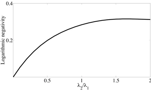
As seen from from Eq. (8), the presence of the driv-ing together with the reservoir demolishes any quantum coherence between the two different parity components. Nevertheless, the steady state will in general be an in-separable state of the atom and the field. To quantify the amount of this bi-partite entanglement present in the atom-field joint density matrix we compute the logarith-mic negativity defined as log(Pn
i |Ξi|), where Pni |Ξi| is
the sum of the absolute values of all the eigenvalues of the partially transposed density matrix [53, 54]. A non-zero value of the logarithmic negativity is sufficient to ensure inseparability of the steady state density matrix ˆ
ρss. The steady state logarithmic negativity, obtained
from numerical integration of the master equation to first obtain ˆρss and then partially transpose it, is plotted as
a function of the dimensionless coupling ratio λ2/λ1 in
Fig. 1. As can be seen, the steady state entanglement between the atom and the field grows with the value of
λ2/λ1. In the limit λ2/λ1 = 0 the case of the
Jaynes-Cummings model is recovered and we know that the steady state is simply ˆρss =|0ih0| ⊗ | ↓ih↓ |. Thus, the
counter rotating terms are responsible for the build-up
of photonic and atomic excitations and thereby also for bi-partite entanglement in the system. However, in the opposite limit, λ1/λ2 = 0, we obtain the
anti-Jaynes-Cummings model and here the steady state is again sep-arable; ˆρss=|0ih0| ⊗ | ↑ih↑ |. A maximum of the
entan-glement should therefore be given for some finiteλ2/λ1,
and from Fig. 1 we see that it happens atλ2/λ1≈1.6, i.e.
it is favourable to support a stronger couplingλ2in order
to achieve a non-classical entangled state. Even though the Jaynes-Cummings and anti-Jaynes-Cummings mod-els are mathematically equivalent (in the bare basis, for example, the Hamiltonian maintains a block structure with 2×2 blocks apart from the ground state), we see that the presence of the Lindblad term ˆLˆaalters this
sym-metry, i.e. the maximum entanglement is not obtained forλ1=λ2.
FIG. 1: (Color online) Steady state entanglement (logarith-mic negativity) in the joint atom-field steady state ˆρss, plotted
here as a function of the dimensionless coupling ratioλ2/λ1.
In the limit of vanishingλ1 or λ2 the steady state is
sepa-rable. The maximum entanglement obtained forλ2 ≈1.6λ1
demonstrates that the presence of photon losses break the symmetry between the Jaynes-Cummings and anti-Jaynes-Cummings models. In particular, the counter rotating terms are responsible for counteracting the losses. The other dimen-sionless parameters are Ω =ω= 1 andγ = 0.1, and for the plot we fixλ1= 0.5.
The reduced density matrix of the boson field is ob-tained by tracing over the atomic degrees of freedom, ˆ
ρfield= Tratom[ˆρss], giving
ˆ
ρfield =
∞ X
n=0
∞ X
m=n,n+2...
P(n, m)|nihm|+h.c. . (10)
As a result of the mixture (8), the steady state field dis-tribution is an individual coherent mixture of even and odd numbered Fock states. However, these two coherent mixtures exist in two different ‘sectors’ with no coherent overlap between them. In Fig. 2 we plot the steady state probability distributionP(n) =hn|ρˆfield|nifor three
dif-ferent values of the ratio λ2/λ1, and again the steady
state has been found by integration of Eq. (6). We find that the steady state density matrix ˆρfield follows
[image:6.612.318.560.245.391.2]FIG. 2: (Color online) Steady state photon probability dis-tributionP(n) for different coupling strengthsλ1 andλ2. It
is noted that the distribution is found to be super-Poissonian in all cases, i.e. the photon distributions alone does not dis-play non-classical features. The lines between the points are for guiding the eye, and the dimensionless parameters are the same as in Fig. 1; Ω =ω= 1 andγ= 0.1.
variance and the mean of the photon number distribution increases with the value of the ratio λ2/λ1. In
particu-lar, and as expected, for increasing atom-field coupling the mean number of photons increases. The counter ro-tating terms play a more important role for this increase to occur. To explore the importance of the bare state coherences in Fig. 3 we plot the absolute value of the first four leading order off-diagonal components of ˆρfield,
namely |P(n, m)| =|hn|ρˆfield|mi|. It is clear that these
imprint the coherence among the bare states belonging to either even or odd parity sectors.
FIG. 3: (Color online) Leading off-diagonal elements of the reduced density matrix ˆρfield (10), when λ2/λ1 = 0.5 (top
row), λ2/λ1 = 1.0 (middle row), and λ2/λ1 = 2.0 (bottom
row), andλ1 = 0.5,0.75,1.0 (increasing from left to right in
all three rows). The alternating zero and non-zero elements reflects the population of states with different parities. The other parameters are the same as for Fig. 2.
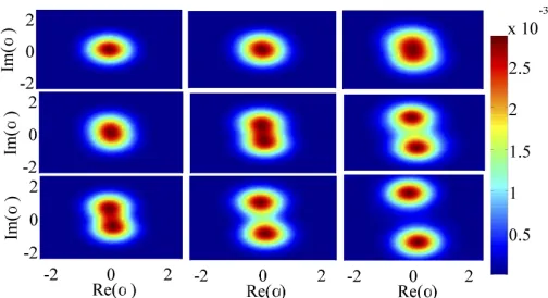
So far we have seen that for the driven/dissipative Rabi model non-classical features may survive. An in-teresting question then raises, which of the features of the (equilibrium) ground state of the Rabi model (6) can be reproduced in the (non-equilibrium) steady state of the master equation (6)? For the Rabi model, in the deep strong coupling regime the ground state becomes a
Schr¨odinger cat [32, 35]. The more resolved the cat state becomes (the smaller the overlap between the two sepa-rated field states in phase space becomes), the higher the atom-field entanglement obtained. More precisely, these ‘dead’ and ‘alive’ field states measure the dipole moment of the atom (corresponding to eigenstates of ˆσx). Thus,
when tracing out the atom, the field state will become a statistical mixture between ‘dead’ and ‘alive’. Note that pure cat state of the form|CAT±i ∝(|αi ± | −αi), for
coherent states| ±αiwith|α|>0, have a definite parity and the corresponding photon distributions contain ei-ther only even or odd photon states|ni. Thus, we ask if we can expect a similar statistical cat also for the reduced density matrix for the boson field (10)? Figure 2 reveals at least that the photon distribution of the steady state is super-Poissonian, and combining this with Fig. 3 one may expect the cat structure to survive photon decay. This should be contrasted with the pioneering experi-ments in theENSParis group which measured the decay of the cat into a fully separable atom-field state before all photons had leaked the cavity [55]. The phase space distribution of the steady state field distribution for the Rabi model is indeed split in two as is shown in Fig. 4. The Wigner function for the field mode can be obtained from the following transformation of the density operator
W(α) = 2
πTr[ ˆD
†(α)ρ
fieldDˆ(α)(−1)ˆa †ˆa
], (11)
where ˆD(α) = exp(αˆa†−α∗ˆa) is the displacement
opera-tor andα=αr+iαmis a complex parameter [56]. Note
that for other expressions for the Wigner function, the real and imaginary parts ofαare related to ‘momentum’
pand ‘position’ x. As can be seen from the figure, on increasing the value of the ratioλ2/λ1the separation
be-tween the two-lobes becomes more pronounced and even-tually the “two-lobes” cease to overlap with each other. A similar two-lobe structure has been found in the tran-sient dynamics of the Wigner function for the dissipative quantum Rabi model with an additional Stark shift term included[29]. For the closed system, this behavior readily follows from a sort of mean-field approach identical to the Born-Oppenheimer approximation [32, 57]. In particular, within this approximation and forγ= 0 the maxima of the Wigner function are found for
Im(α) =
0, g≤gc
±qωg22 −
Ω2
16g2, g > gc
, (12)
whereg= (λ1+λ2)/2 andgc=
√
ωΩ/2, and Re(α)≡0. Note that gc coincide with the critical coupling of the
Dicke model [36]. Thus, the splitting grows approxi-mately linear withλ1+λ2. If the signs of the couplings λ1 and λ2 are different the roles of the real and
[image:7.612.57.301.53.168.2] [image:7.612.56.310.417.544.2]anti-clockwise tilting of the Wigner function. This is a result of the Lamb shift [56], i.e. it only arises due to the coupling to the bath. This is also easily understood by considering the mean-field versions of the Heisenberg equations of motion for the open Rabi model. The steady state solution for the field will then include a non-zero imaginary part (or real part depending on how one de-fines α) which implies that the field phase for the sepa-rated blobs is not exactly±π[58].
FIG. 4: (Color online) Steady state Wigner function (11) for the anisotropic Rabi model; λ2/λ1 = 0.5 (top row), Rabi
model λ2/λ1 = 1.0 (middle row), andλ2/λ1 = 2.0 (bottom
row), andλ1 = 0.5,0.75,1.0 (increasing from left to right in
all three rows). The splitting between the two blobs scale as λ1+λ2for the closed case. The presence of photon loses tend
to make the splitting smaller since the corresponding Lindblad term favor a vacuum state. The bath also brings about an energy (Lamb) shift which is manifested in the tilting of the Wigner function. The absence of negativity of the Wigner functions in this plot does not solely result from the reservoir induced decoherence but also from the entanglement shared between the atom and the field. The other parameters are the same as for Fig. 2.
III. MODEL B - ANISOTROPIC DICKE MODEL (NORMAL PHASE)
The Rabi model is highly quantum in the sense that quantum fluctuations play a dominant role in the spin sub-space, and consequently it lacks a natural classical limit. Such a limit would, however, emerge if we allow the spin to become very large, i.e. the Pauli matrices are replaced by general angular momentum operators ˆSα
(α= x, y, z). In doing this replacement we obtain the anisotropic Dicke model (ADM)
ˆ
HADM=ωˆa†ˆa+
Ω 2Sˆz+λ1
ˆ
a†Sˆ−+ ˆS+ˆa+λ2
ˆ
a†Sˆ++ ˆS−aˆ.
(13) It is the purpose of this section to demonstrate that non-classicality of the steady state survives also in this clas-sical limit.
With the correct scaling of the coupling parameters (relative to the system size), the Dicke model is critical
with the normal phase characterized by a vacuum photon field and the spin pointing towards the south pole. The superradiant phase instead comprises a coherent photon state and the spin rotated away from the south pole [36]. True criticality only emerges in the thermodynamic limit meaning that the spin S → ∞ [60]. In the strict limit of infinite spin, the spectrum is linear and we may re-place spin operators by boson operators (plus an overall energy shift). In such a case we consider the following Hamiltonian
ˆ
HnAD=ωˆa†aˆ+ Ωˆb†ˆb+λ1
ˆ
a†ˆb+ ˆb†aˆ+λ2
ˆ
a†ˆb†+ ˆbˆa,
(14) where the notation HˆnAD refers to the linearized
anisotropic Dicke model in the normal phase. Clearly the above Hamiltonian can be used to model various other physical systems, including coupled harmonic os-cillators/cavity modes [49]. Going from the non-linear model (13) to the linear approximated model (14) al-lows for an analytical approach. For finite systems the non-linearity will enter after sufficiently long times [61]. Here, however, we assume that this time-scale is much longer than the intrinsic relaxation time of the open sys-tem, i.e. we push any quantum revivals to happen be-yond our experimental times. In the normal phase of the Dicke model, the linear Hamiltonian ˆHnADdescribes
the collective quantum excitations/fluctuations (Bogoli-ubov modes) [15]. This is most easily seen by linearizing the original Dicke model in the Holstein-Primakoff boson representation [15, 60]. In the superradiant phase, the re-sulting quadratic boson Hamiltonian contains additional squeezing terms, e.g. ˆb2 and ˆa2[62]. Within the effective
linear model, the quantum fluctuations cause entangle-ment in the system, and for the closed Dicke model it has been found that the atom-field entanglement peaks at the critical point [63]. We point out, however, that since the Lindblad jump operator [ˆa,HˆADM]6= 0 it is not,
in principle, clear that criticality of ˆρss is preserved in the
presence of the photon decay. This issue was recently ad-dressed and photon losses do not destroy criticality but alters both the critical coupling and the critical expo-nents [15, 59]. As discussed in more details below, the conservation of the critical point under photon losses can be understood from the fact that the state for the normal phase is actually a dark state of the Lindblad operators. Here, as we are interested in the opposite (classical) limit of the Rabi model, we only consider the fluctuations in the normal phase and not in the superradiant one. This emerges in the present analysis as destabilization of the Bogoliubov modes upon approaching the critical point.
Going beyond the study in [63], we here include the interaction with the outside environment. We again en-visage a scenario where damping of the field mode is the only dominant dissipation channel;
˙ˆ
ρ=−i[ ˆHnAD,ρˆ] +γLˆaρ.ˆ (15)
[image:8.612.55.307.165.302.2]assump-FIG. 5: Stability criterion ζ (17) for different values of the ratio λ2/λ1, shown here as a function of the decay rate of
the field modeγand the coupling strengthλ1. The non-zero
valueζ6= 0 mark the transition to the unstable regime. The dimensionless atomic and field frequencies Ω =ω= 1.
tion can be justified if it is possible to realize the ADM (14) through a scheme outlined in [15]. Specifically, mode ˆb can play the role of collective Bogoliubov excitations of a collection of level” systems, where each “two-level” system can be the metastable low lying energy dou-blet of a Raman driven four level atom. Also, as discussed in the previous section, a phenomenological introduction of the Lindblad super operator for the field mode as in-troduced in the master equation (15) can only be jus-tified for an original time-dependent Hamiltonian. It is worth pointing out that for a time-independent model described by the Hamiltonian (14) a correct description of the open dynamics results in a non-local master equa-tion which disagrees with the predicequa-tions of the master equation (15) [49].
As already mentioned, since the Hamiltonian is quadratic we may approach the problem analytically. To this end we define the two-mode normal-ordered char-acteristic function χ(ǫa, ǫb, t) = heǫaˆa
† e−ǫ∗
aˆaeǫbˆb†e−ǫ∗bˆbi.
From the quantum characteristic function the complete statistical description of the corresponding state can be obtained. One can therefore obtain the expectation val-ues of quantum mechanical observables, e.g. for the equal time correlator one has
hˆa†m(t)ˆb†n(t)i
=
∂
∂ǫa
m ∂
∂ǫb
n
χ(ǫa, ǫ∗a, ǫb, ǫ∗b,t)|ǫa,ǫ∗a,ǫb,ǫ∗b=0.
For an initial Gaussian state of the two modes ˆaand ˆb, the master equation (15) can be expressed as a partial differential equation forχ[49]
∂ ∂tχ=z
TMzχ+zTN
[image:9.612.65.289.56.230.2]∇χ, (16)
FIG. 6: Bi-partite entanglement between the modes ˆa and ˆbfor three different valuesλ2/λ1 and as a function ofγ and
λ1. Right before the solution gets unstable (white region, and
see previous figure 5) the entanglement is maximized. This is in agreement with the fact that in the full Dicke model this marks a critical point [63]. Note, however, that the critical point has been shifted due to the coupling to the bath. The remaining dimensionless parameters are Ω =ω= 1.
wherezT = (ǫ
a, ǫ∗a, ǫb, ǫb∗),∇= (∂ǫ∂a, ∂ ∂ǫ∗
a, ∂ ∂ǫb,
∂ ∂ǫ∗
b) T and
M =
0 0 iλ2/2 0
0 0 0 −iλ2/2 iλ2/2 0 0 0
0 −iλ2/2 0 0
,
N =
iω−γ 0 iλ1 −iλ2
0 −iω−γ iλ2 −iλ1 iλ1 −iλ2 iΩ 0 iλ2 −iλ1 0 −iΩ
are the drift and diffusion matrices respectively. We first analyze the steady state solution of the master equa-tion (15). In particular, the soluequa-tion is stable if the real parts of all the eigenvalues of the diffusion matrixNare
all negative. In particular, when Ω =ω, the stability of the steady state requires
ζ= Maxℜ(±ν+,
±ν−)
−γ <0, (17)
where,
ν+ =
s
γ2−4
λ2
1−λ22+ω2+
q
4λ2
1ω2−γ2ω2
,
ν− =
s
γ2−4
λ2
1−λ22+ω2−
q
4λ2
1ω2−γ2ω2
.
The stability parameterζis shown in Fig. 5 as a func-tion of the damping rate of the field modeγand the two-mode coupling strengthλ1. As is evident from the figure,
[image:9.612.325.551.57.229.2]steady state to be achieved for an extended region of pa-rameter space spanned byλ1. This behavior can be
un-derstood physically by considering the different terms of the master equation (15). First we may note that the in-stability of the mode coincides with the Dicke phase tran-sition. Indeed, the model Hamiltonian (14) describes the collective excitations in the normal phase and not in the superradiant phase, and hence, these excitation modes cannot be analytically continued into the superradiant phase. Thus, we conclude that increasing the photon loss gives a more extended normal phase. This is expected since the Lindblad term of Eq. (15) favors the vacuum state of the field, which is also favored by the bare field energyωˆa†ˆa. On the other hand, the atom-field coupling
term is not minimized by such a field state. Without pho-ton decay, the transition occurs at (λ1+λ2) =√ωΩ (see
Eq. (15)), but now losses support the normal phase and thereby shift the critical value. Following Refs. [15, 64] one explicitly findsλc=
p
Ω (ω2+γ2)/ω/2 which is
ob-tained at the mean-field level, i.e. in the thermodynamic limit. In the Dicke limit (λ1=λ2=λ) it is easy to obtain
the phase boundary ω2+γ2 = 4λ2, which retrieves the
result for the critical coupling of the open Dicke model on resonance [15, 64].
The steady state of light-matter coupled quantum sys-tem modeled under the master equation (6) was shown to be an inseparable state of the cavity field and the two-level system. Somewhat surprisingly, this observa-tion can also be extended to the steady state of the normal phase of the Dicke model (15). In particu-lar, one could argue that in the thermodynamic limit as studied here any entanglement should vanish since for the Dicke model quantum fluctuations are negligi-ble [65]. That this is not the case derives from the pres-ence of the critical point. To demonstrate sustainable quantum correlations we next evaluate the steady state bi-partite entanglement between the two modes ˆa and ˆb and characterize it in terms of the logarithmic neg-ativity which for two-mode Gaussian states serves as a necessary and sufficient criterion for the inseparabil-ity [66]. A two-mode Gaussian state can be fully quanti-fied in terms of its covariance matrixVwhich is a 4×4
symmetric matrix with Vij = (hRiRj +RjRii)/2 and
RT = (ˆq
a,pˆa,qˆb,pˆb). Here ˆqa,b and ˆpa,b are the
posi-tion and momentum quadratures of the mode ˆa(ˆb). For a two-mode Gaussian continuous-variable state with co-variance matrixV, the logarithmic negativity is obtained
asN = Max[0,−log(2ν−)] [66], whereν− is the smallest
of the symplectic eigenvalues of the covariance matrix, given byν−=
q
σ/2−p
(σ2−4DetV)/2. Here σ = DetA1+ DetB1−2DetC1
V =
A 1 C1 CT
1 B1
,
whereA1 (B1) accounts for the local variances of mode
a(b) and C1for the inter-mode correlations. Using the
numerical solutions of the partial differential equations
(16) we compute the logarithmic negativity. The steady state two-mode entanglement is shown in Fig. 6 where it is given as a function of the damping rateγ and the two-mode coupling strengthλ1. As is evident, the
maxi-mum attainable bi-partite entanglement between the two modes monotonically increases on increasing the value of the ratio λ2/λ1. The highest entanglement is
ob-tained at the critical point, which is also known from the closed Dicke model [63]. This is, in fact, a general property for quantum phase transitions; at the critical point where characteristic length scales diverge, the en-tanglement also diverges [67]. However, already for the closed Dicke model the phase transition is not a ‘typical’ quantum phase transition since there is no length scale in the problem and, as we mentioned above, quantum fluctuations vanish in the thermodynamic limit. Because of this, the transition has been called ‘classical’ [65]. As such, the results of Fig. 6 suggest that, qualitatively, the same behavior of the entanglement is found for a dynam-ical phase transition of an open driven system.
[image:10.612.317.572.347.445.2]IV. QUANTUM CONTROL IN HYBRID ARCHITECTURES
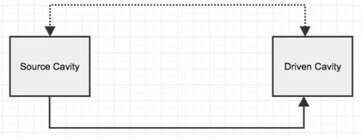
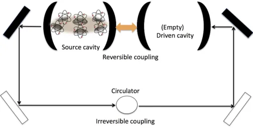
FIG. 7: Schematic plot of the feedback loop between the two cavities. We envision a scenario of two coupled cavities; a source cavity and a driven cavity. The driven cavity is as-sumed to be slaved to the source cavity. The source cavity drives the state of the slave cavity by means of a unidirec-tional coupling (shown by a solid line). The driven cavity in turn also influences the state of the source cavity by means of a reversible interaction (shown by a dotted line). The si-multaneous presence of reversible and irreversible couplings between the cavity modes results in an all-optical feedback loop.
In the previous two sections we have studied the open dynamics of the anisotropic Rabi and Dicke models and have explicitly explored the properties of the NESSs of these models. However, so far we have eluded ourselves from effectively engineering the open dynamics of these hybrid models. Even though it was found that entangle-ment persists in both models despite losses, in the present section we wish to explore the possibilities to enhance the amount of entanglement by actively introducing feedback into the model.
FIG. 8: Illustration of the general all-optical feedback of Fig. 7 specifically used for establishing quantum control in the Dicke model of Section III. The internal dynamics of the source cav-ity is modeled by (14) while the driven cavcav-ity is initially pre-pared in its vacuum state. Mode ˆaof the source cavity and the mode ˆcof the driven cavity are interacting under a re-versible interaction of the form (18). Mode ˆa of the source cavity also couples irreversibly to mode ˆcof the driven cav-ity. Such afeed-forwardcoupling can be engineered through feeding the mode ˆa from one end of the source cavity and reflecting it onto the driven cavity through a series of mirrors (filled) and beam-splitters (unfilled). Optical circulators or Faraday isolators can be used to prevent interference from re-flections in the opposite directions. Reversible and irreversible interactions jointly constitute an all-optical feedback. If this feedback loop has negligible time delay a Markovian master equation to describe the open dynamics of the source cavity can be derived (21) as detailed in Section IV A.
result in exotic NESS properties [9, 11, 48, 68, 69]. This was in particular the theme of the previous two sections. However, engineering a controlled degree of dissipation is also an important tool in realizing tasks of quantum information processing. In this spirit we will now use an all-optical feedback scheme for quantum state protection and establishing quantum control in the normal phase of the Dicke model. The scheme we choose is based on coherent feedback, i.e. no measurement is performed in the feedback loop [16]. A symbolic plot of a coherent (all-optical) feedback scheme is illustrated in Fig. 7; it comprises of two units, which have been labeled source and driven cavities, with reversible and irreversible cou-plings between them. The simplest all optical feedback loop will use the output from a source cavity and feedfor-ward into a driven cavity which is coupled to the source cavity in some way. It is worth mentioning that unidirec-tional and bidirecunidirec-tional couplings between the source and the driven cavities jointly constitute an all optical feed-back scheme. A coherent feedfeed-back loop, however, can also introduce a finite time-delay τ. Firstly, assuming that the time-delayτ introduced by the feedback loop is negligible, we study the open dynamics of the source cav-ity [18–20]. Subsequently, making use of a time-delayed feedback control method, [21–23] we incorporate a time-delayτ introduced by the feedback loop.
A. All optical feedback loop with negligible time-delay τ
We now apply the general scheme of all-optical feed-back illustrated in Fig. 7 for a specific task of quantum state protection in the anisotropic Dicke model of Sec. III. A schematic of our proposal to implement all-optical feedback is shown in Fig. 8. The internal (unitary) dy-namics of the source cavity is described by the Hamilto-nian (14), i.e. ˆHsource= ˆHnAD and the driven cavity is
reversibly coupled to the field mode of the source cavity by the following Hamiltonian [18, 19]
ˆ
Hint=iµ
√γγ
d
2 (ˆa
†cˆ
−ˆc†ˆa), (18)
whereµis a dimensionless coupling parameter, ˆc† and ˆc
are the creation and annihilation operators for the field mode of the driven cavity which has damping rate γd.
The driven cavity is assumed to be prepared in its vac-uum state with its respective internal dynamics modeled as ˆHdriven= Ωdcˆ†ˆc. A reversible interaction of the form
(18) can arise through mode overlap between the modes ˆ
aand ˆc [70].
Under the Born-Markov approximation a joint state of the source and driven cavities, represented here as ˆW, evolves under the following master equation [16, 18, 19]
˙ˆ
W = −ihHˆnAD+Hdriven+ ˆHint,Wˆ
i
+√γγd([ˆaW ,ˆ ˆc†] + [ˆc,W aˆ †])
+γ
2LaˆWˆ +
γd
2 LˆcW .ˆ (19) It should be remarked that ˆW represents a tri-partite state of modes ˆa,ˆb, and ˆc. On the grounds of arguments presented previously, we have again neglected damping of the mode ˆb of the source cavity. The two terms ap-pearing in the second line account for the unidirectional coupling between the source and driven cavities and the last two terms are the individual Lindblad operators de-scribing photon losses for the source and driven cavity modes respectively. As illustrated in Fig. 8, such a uni-directional coupling between the source and driven cavi-ties can be established using an optical circulator [18]: a non-reciprocal optical device such as Faraday rotator can be used to establish irreversible coupling between the op-tical modes ˆaand ˆcof the source and the driven cavities. As pointed out in Refs. [18, 19], for the feedback loop to be effective the driven cavity should respond much faster than the source cavity. We thus work in a regime where
γd ≫ 1 meaning that the state of the driven cavity is
slaved to the state of the source cavity. Since γd is the
cavities as
ˆ
W = ˆρ00|0ih0|+ ˆρ10|1ih0|+ ˆρ†10|0ih1|
+ˆρ11|1ih1|+ ˆρ20|2ih0|+ ˆρ†20|0ih2|, (20)
where ˆρij is the conditional state of the source cavity
(a joint state of modes ˆaand ˆb) when the driven cavity is projected on the state space |iihj|. Using the above ansatz and adiabatically eliminating the driven cavity it is possible to derive an effective master equation for the source cavity alone [18, 19]. Following the derivation pro-vided in Appendix A one arrives at the resulting master equation
˙ˆ
ρ = ˙ˆρ00+ ˙ˆρ11=−i
h
ˆ
HnAD,ρˆ
i
+γeff
2 Lˆaρ,ˆ (21) where γeff =γ(1 +µ(2 +µ)) is the new effective
damp-ing rate of the field mode. On choosdamp-ing the dimensionless parameter µ =−1, it is remarkable to observe that an all optical feedback loop is capable of completely block-ing the loss of the source cavity. However, losses in the feedback loop would deteriorate the effectiveness of such feedback. If the feedback loop has an efficiency
η (≤ 1), then it is possible to show that the effec-tive damping rate of the source cavity gets modified as
γeff =γ(1 +ηµ(2 +µ)) [19]. We therefore conclude that,
under the assumptions that the time-delay introduced by a feedback loop is negligible and the state of the driven cavity is effectively slaved to the source cavity, it is pos-sible to establish arbitrary control over the damping rate of the source cavity. This can be an important step for quantum state protection in hybrid quantum systems.
As an example application of an all optical feedback scheme for quantum state protection, we assume that the two coupled modes interacting under the Hamiltonian (14) are initially prepared in a NOON state [71]. NOON states are Bell-like entangled states with applications in quantum metrology and quantum lithography and they may also be utilized for achieving phase supersensitivity [72]. We assume that the modes ˆa and ˆb are initialized in a state|ΨN
−i= (|Nia|0ib− |0iaNib)/
√
2. We examine the autocorrelation function, i.e. the overlap between ˆ
ρ(0) and the time evolving joint state of the two modes ˆ
ρ(t), which for mixed states is given by the Uhlmann fidelity [73, 74]
Φ = Tr
q p
ˆ
ρ(0)ˆρ(t)pρˆ(0). (22)
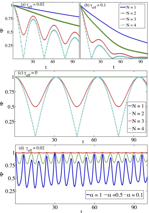
The time evolution of the fidelity Φ for different values ofN and two different values ofγeff is plotted in Fig. 9
(a) and (b). We note that the results are for a small coupling (20λ1 = 20λ2 =ω= Ω) in order to assure
nu-merical convergence. In Fig. 9 (c) we also show the time evolution of the fidelity Φ for an initial bi-model NOON state in absence of photon losses. As is evident, by con-trolling the damping rate of the source field it is possible to prolong the lifetime of the initially prepared NOON state. It follows that suitably choosing γeff allows the
FIG. 9: (Color online) The upper plots (a) and (b) give the time evolution of the fidelity Φ for a bi-modal NOON state in the presence of losses, while (c) shows the same but in ab-sence of photon losses. By comparing the first two examples it is clear that the feedback loop makes it possible to preserve coherent evolution for longer times. The last plot (d) is the same but for an entangled cat state with one mode in vacuum and the other in a coherent state|αi. The shorter period re-sults from the dephasing of the different Fock states involved. The other dimensionless parameters are Ω =ω= 1, λ1= 0.05
andλ2/λ1= 1 in all four panels.
value of the fidelity to be kept above its classical value of 2/3 [75] for a longer time. It is also worth noting that NOON states become more susceptible to the environ-mental damping with the increase in the excitation num-ber N. In this scenario establishing a control over the damping rate of the field in the source cavity could be an important step in preserving initial quantum coherence. In the Appendix B we analytically analyze the structure of especially plot (c), and explain why the fidelity stays constant forN= 1,2 and not forN = 3,4.
Also shown in Fig. 9 (d) is the evolution of the Uhlmann fidelity of a two-mode entangled coherent state |Ψi = (|αia|0ib +|0ia|αib)/
p
2(1 +e−|α|2
[image:12.612.319.563.49.397.2]exhibit noticeable improved sensitivity for phase estima-tion when compared to that for NOON states. Entangled coherent states can also outperform the phase enhance-ment achieved by NOON states both in the lossless, weak, moderate and high loss regimes [76]. As demonstrated in Fig. 9 (d), when compared to a NOON state a two-mode entangled coherent state is found to be more resilient to photon losses. Nevertheless, the quantum fidelity of en-tangled coherent states also seems to decay significantly with the increase in the mean number of photons|α|2.
B. All optical feedback loop with finite time-delay τ
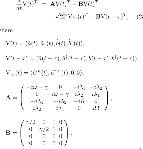
As mentioned before, in deriving the master equation (21) it has been assumed that the time-delay τ intro-duced by the feedback loop is negligible [18]. In this section we explore a complementary regime when the feedback loop introduces a non-negligible time-delay τ. In particular, we use the time-delayed feedback control method of Ref. [21–23] and apply it to our Hamiltonian (14). We refer the reader to [23] for a specific proposal implementing a finite time-delay in an optical feedback loop and applying it to the Dicke model (14). In this work we go beyond the analysis presented in [23] and will include quantum fluctuations to check the steady state stability of the time-delayed feedback control scheme and to compute steady state correlations between modes ˆa,ˆb. Considering a specific all-optical time-delayed feedback control strategy discussed in detail in [23] and apply-ing it to our Hamiltonian (14) we arrive at the followapply-ing Heisenberg-Langevin equations of motion (14)
d dtV(t)
T = AV(t)T
−BV(t)T
−√2Γ Vin(t)T+BV(t−τ)T, (23)
where
V(t) = (ˆa(t),ˆa†(t),ˆb(t),ˆb†(t)),
V(t−τ) = (ˆa(t−τ),ˆa†(t
−τ),ˆb(t−τ),ˆb†(t
−τ)),
Vin(t) = (ˆain(t),aˆ†in(t),0,0),
A=
−iω−γ 0 −iλ1 −iλ2
0 iω−γ iλ2 iλ1
−iλ1 −iλ2 −iΩ 0 iλ2 iλ1 0 iΩ
,
B=
γ/2 0 0 0 0 γ/2 0 0 0 0 0 0 0 0 0 0
.
(24) Here,Vin(t) contains the input noise terms [77]. It should
be pointed out that in writing the above
Heisenberg-Langevin equations we have assumed that the time-delayed feedback loop has unit efficiency [23]. To con-nect with the approach of the previous sections, we have again assumed that the damping of the mode ˆais the only dominant channel of dissipation. Also, the time-delayed control feedback strategy (23) is implemented through a control force which is generated from the difference be-tween the instantaneous cavity field ˆa(t) and the field at some point in the past ˆa(t−τ) [23].
As a first step to check the influence of the time-delayed feedback control on our hybrid quantum system we check the stability of the above Heisenberg-Langevin equations semi-classically,i.e. we assume the noisehVin(t)i=0.
Us-ing an ansatz V(t) ∼ eΛt we get the following secular
equation [21, 22]
det(A−B+Be−Λτ−Λ1). (25)
For a non-zero value of τ, this transcendental equation has an infinite set of complex solutions for eigenvalues Λ. The steady state is stable only if the real parts of all the solutions Λ are negative [21, 22]. We numerically solve the above secular equation (25) for all possible roots Λ. In doing so we chooseλ1andγ such that in the absence
of a time-delayed feedback loop the steady state is stable for all values of the ratio 0≤λ2/λ1 ≤2, see Fig. 5. In
Fig. 10 we plot the maximum of the real part of all possi-ble solutions Λ. We find that at a semiclassical level, and for the set of parameters considered in Fig. 10, our time-delayed feedback control strategy does not qualitatively alter the stability of the steady state.
FIG. 10: (Color online) Maximum of the real part of all pos-sible solutions of the secular equation (25) for three different values of the ratio λ2/λ1 and shown here as a function of
the time-delay τ. The dimensionless parameters have been taken Ω = ω = 1, λ1 = 0.1 and γ = 0.1. For these set of
parameters the steady state is stable for all values of the ra-tio 0≤λ2/λ1 ≤2 in the absence of a time-delayed feedback
loop, see Fig. 5.
[image:13.612.321.552.422.531.2] [image:13.612.59.292.451.693.2]two-FIG. 11: (Color online) The upper plot (a) displays the bi-partite entanglement (negativity) between the modes ˆaand ˆb as a function of the dimensionless ratioλ2/λ1 and the
time-delay τ, and in the lower plot (b) the entanglement is given for different ratiosλ2/λ1 and for different choices ofτ. Also
shown in (b) is the steady state bi-partite entanglement be-tween the modes ˆa and ˆb in the absence of a time-delayed feedback loop, and we especially note that by introducing a time-delay the amount of entanglement can be increased. In the black region in (a) the solution does not approach a phys-ical steady state. The dimensionless parameters have been taken Ω =ω= 1, λ1= 0.1 andγ= 0.1.
mode covariance matrix in order to capture the quan-tum correlations between the modes ˆa and ˆb. We then evaluate the bi-partite entanglement (logarithmic nega-tivity) between the two modes ˆaand ˆb. In Fig. 11 (a) we display the bi-partite entanglement between the modes ˆ
a and ˆb as a function of the dimensionless ratio λ2/λ1
and the time-delay τ. As for Fig. 10, we choose λ1 and γ such that in the absence of a time-delayed feedback loop the steady state is stable for all values of the ratio 0≤λ2/λ1≤2. We find that for a fixed value of the
time-delay τ the bi-partite entanglement between the modes ˆ
aand ˆbincreases with the value of the ratio λ2/λ1, this
is expected since the coupling between the two modes is also increased. However, we also observe that there is a “delay-window” (shown in black and labeled ‘Unphysi-cal’ in Fig. 11 (a)), such that if τ is chosen within this interval then a physical steady state is never reached [79]. We also find that a suitable choice of the time-delay can also increase the steady state bi-partite entanglement be-tween the modes ˆa and ˆb. More precisely, the bi-partite entanglement between the modes ˆa and ˆb for different
choices of τ is given in Fig. 11 (b), where for the sake of elucidating the role of time-delayed feedback loop we have also shown the steady state entanglement between the modes ˆaand ˆbin the absence of a time-delayed feed-back loop.
V. CONCLUSIONS
In this work we have studied two topical hybrid sys-tems, the anisotropic Rabi and Dicke models, both of which combine disparate quantum degrees of freedom; light and matter. While similar, the two models oper-ate in different ‘regimes’; the Rabi model displays large quantum fluctuations which is not the case of the Dicke model. We have first explored the open dynamics of a two-level system (a model atom) strongly coupled to a boson (photon) field, i.e. the Rabi model. We have shown that the NESS is an entangled state of the light and atom systems. More precisely, the steady state is a statistical mixture of two states with opposite parities. In phase space these even and odd parity states forms a cat-like structure, which however gets ‘tilted’ due to the reservoir-induced Lamb shift. As a second physical model we have investigated two coupled boson modes which can describe linearized interactions between a cav-ity field and a collection of two-level systems in the ther-modynamic limit, i.e. the Dicke model. This linearized version of the anisotropic Dicke model describes the col-lective excitations in the normal phase. We have espe-cially explored the stability and bi-partite entanglement in this second physical setting, again in the presence of coupling to an environment. Even though quantum fluc-tuations are negligible in the thermodynamic limit, en-tanglement survives which we attribute to the presence of a critical point which persists also under dissipation. As a way to establish quantum control and increase non-classical properties in such hybrid quantum architectures, we propose to use an all optical feedback strategy. We demonstrated this approach by utilizing the scheme for the Dicke model, for two applications. We have applied feedback to provide protection (against loss) of quantum states of interest for metrology (NOON and entangled coherent states). We have also demonstrated that a re-alistic feedback proposal including a time-delay can be used to alter the properties of the NESS potentially in-creasing the entanglement between the sub-systems and changing the stability of the steady state.
Acknowledgments
[image:14.612.55.297.51.305.2]Appendix A: Markovian master equation with optical feedback
In this appendix we provide the details of the deriva-tion of the master equaderiva-tion (21). For the feedback loop to be effective, the driven cavity should respond much faster than the source cavity. We thus work in a regime where
γd≫1 and the state of the driven cavity follows
adiabat-ically the evolution of the source cavity. The large decay rate and the coupling to a zero temperature reservoir implies that driven cavity may only be weakly excited, which justifies the ansatz state (20). With such a joint state of two coupled cavities one obtains the following equations of motion for the source cavity
˙ˆ
ρ00 = −i
h
ˆ
HnAD,ρˆ00
i
+γ
2Laˆρˆ00+γdρˆ11 +√γγd(ˆaρˆ10† + ˆρ10ˆa†) +µ
√γγ
d
2 (ˆa
†ρˆ
10+ ˆρ†10ˆa)
˙ˆ
ρ10 = −i
h
ˆ
HnAD,ρˆ10
i
+γ
2Laˆρˆ10−
γd
2 ρˆ10 +√γγd(ˆaρˆ11−ˆaρˆ00+
√ 2ˆρ20ˆa†)
+µ √γγ
d
2 ( √
2ˆa†ρˆ
20−ˆaρˆ00+ ˆρ11ˆa)
˙ˆ
ρ11 = −i
h
ˆ
HnAD,ρˆ11
i
+γ
2Laˆρˆ11−(iΩd+γd)ˆρ11 −√γγd(ˆaρˆ10† + ˆρ10ˆa†)−µ
√γγ
d
2 (ˆaρˆ
†
10+ ˆρ10ˆa†)
˙ˆ
ρ20 = −i
h
ˆ
HnAD,ρˆ20
i
+γ
2Laˆρˆ20−2γdρˆ20 −p
2γγdaˆρˆ10−µ
√γγ
d
√ 2 ˆaρˆ10.
The state of the source cavity is of interest to us and it can be extracted as ˆρ= TrˆcW = ˆˆ ρ00+ ˆρ11. From the
above equations, the off-diagonal elements ˆρ10 and ˆρ20
can be adiabatically eliminated by slaving them to the diagonal elements ˆρ00 and ˆρ11. Setting ˙ˆρ20=0 we obtain
to leading order in 1/p(γd/γ)
ˆ
ρ20=−
1
p
2(γd/γ)
(µ
2 + 1) ˆaρˆ10. (A1) Inserting the above expression in the steady state equa-tion of ˆρ10 we obtain
ˆ
ρ10=
2
p
(γd/γ)
(µ 2ρˆ11ˆa−
µ
2ˆaρˆ00+ ˆaρˆ11−ˆaρˆ00). (A2) Using the above steady state solution for the off-diagonal element yields the following master equation for the den-sity matrix of the source cavity alone
˙ˆ
ρ = ˙ˆρ00+ ˙ˆρ11=−i[ ˆHnAD,ρˆ] + γ
2Laˆρˆ−iΩdρˆ11 +µγ[Laˆ(ˆρ00−ρˆ11) +
µ
2Laˆρˆ00+
µ
2Lˆa†ρˆ11].(A3) When γd ≫ 1, ˆρ11 ∼ O(0) and ˆρ ≈ ρˆ00 we arrive at
the following master equation approximating the source
dynamics
˙ˆ
ρ = ˙ˆρ00+ ˙ˆρ11=−i
h
ˆ
HnAD,ρˆ
i
+γeff
2 Lˆaρ,ˆ (A4) whereγeff =γ(1 +µ(2 +µ)) is the effective damping rate
of the field mode in the source cavity.
Appendix B: Uhlmann fidelity in the RWA regime
A conspicuous feature of Fig. 9 (especially in (c)) is the almost constant evolution of the fidelity for the states with N = 1,2, and the oscillatory structure for the
N = 3, 4 states. This implies that |Ψ1−,2i are
station-ary states while|Ψ3−,4iseems to be formed from two sta-tionary states. In this appendix we will explain how this comes about given the initial states and the Hamiltonian (14). As pointed out in the main text, for the figure a small coupling has been used (20 times smaller than the bare frequencies) which means that imposing the RWA is justified, i.e. we let λ2 = 0 from now on. We have
numerically verified that the RWA is applicable for the corresponding parameters.
Now, when λ2= 0 the Hamiltonian can be readily
di-agonalized by defining two new bosonic operators; ‘even’ ˆ
z+ = (ˆa+ ˆb)/
√
2 and ‘odd’ ˆz− = (ˆa−ˆb)/
√
2. These obey the regular boson commutation relations and mu-tually commute. In particular the ‘odd’ Fock states |n−i = ˆz
†n−
− |0i/ p
n−! have shown to be important for
adiabatic passage in multimode cavities [78]. Expressed with the new rotated operators, the Hamiltonian is diag-onal
Hz= (ω+λ1)ˆz†+zˆ++ (ω−λ1)ˆz−†zˆ−. (B1)
It follows that the eigenstates are |n+i|n−i =
ˆ
z†n+
+ zˆ
†n−
− |0ia|0ib/ p
n+!n−!, with corresponding
eigenen-ergiesεn+n− =ω(n++n−) +λ1(n+−n−).
For anN particle NOON state we have
|ΨN−i=
1 √
2N!
ˆ
a†N−ˆb†N|0ia|0ib. (B2)
Thus, we notice that|Ψ1
−i= ˆz †
−|0ia|0ib is indeed a
sta-tionary state with its time evolution given by
|Ψ1−(t)i=e−i(ω−λ1)t|Ψ1−i. (B3)
The time evolved state (B3) is of course strictly only cor-rect within the RWA, and the exact time evolved state should be given by evolution under the full Hamiltonian; |Ψ1
exact(t)i=e−i ˆ
HnADt|Ψ1
−i. Numerically we find the
er-ror arriving from neglecting the counter rotating terms
δ1=|Φexact−ΦRWA|<0.003 for allt. Similarly, we find
that the two particle NOON state|Ψ2
−i= ˆz †
+zˆ
†
−|0ia|0ib
is also a stationary state with the time evolution