A sparse kernel density estimation algorithm using forward constrained regression

using Forward Constrained Regression

Xia Hong†_{, Sheng Chen}‡_{, and Chris Harris}‡

†_{School of Systems Engineering, University of Reading, Reading, RG6 6AY, UK} ‡ _{School of Electronics and Computer Science, University of Southampton,}

Southampton SO17 1BJ, UK

Abstract. Using the classical Parzen window (PW) estimate as the tar-get function, the sparse kernel density estimator is constructed in a for-ward constrained regression manner. The leave-one-out (LOO) test score is used for kernel selection. The jackknife parameter estimator subject to positivity constraint check is used for the parameter estimation of a single parameter at each forward step. As such the proposed approach is simple to implement and the associated computational cost is very low. An illustrative example is employed to demonstrate that the proposed approach is effective in constructing sparse kernel density estimators with comparable accuracy to that of the classical Parzen window estimate.

Key words: cross validation, jackknife parameter estimator, Parzen window, probability density function, sparse modelling.

1

Introduction

A basic problem that is pertinent to many machine learning and pattern recog-nition applications is to estimate the probability density function (pdf) from observed data samples [1–4]. A general and powerful approach to the problem of probability density function estimation is the finite mixture model [5]. The finite mixture model includes the well known PW estimate [4] as a special case. It is useful to develop methods of fitting a finite mixture model with the capability to infer a minimal number of mixtures from the data efficiently. Re-searches into sparse density estimators include the support vector machines[6, 7], the reduced set density estimator (RSDE) [8], and sparse pdf estimator using forward orthogonal regression (OFR) [9–11].

to a simple positivity constraint. A one parameter jackknife parameter estima-tor is utilized in each regression step, subject to the same positivity constraint check. The proposed algorithm has the advantage of maximal computationally efficiency due to that (i) the parameter estimation is reduced to the solution of the minimal possible number of one parameter; and (ii) the positivity constraint on the mixing weights can be easily accommodated.

2

The Kernel Density Estimator

Given a finite data set consisting of N data samples, D = {x1, ...,xj, ...xN},

where the feature vector variablexj ∈ <m follows an unknown probability

den-sity functionp(x), the problem under study is to find a sparse approximation of p(x) based onD.

A general kernel based density estimate ofp(x) is given by

ˆ

p(x;g, σ) =PN

j=1gjK(x,xj) (1)

subject to gj ≥0, j= 1, ..., N, gT1= 1.

where g = [g1, g2, ..., gN]T. gj’s are the kernels weights. 1 is a vector with an

appropriate dimension and all elements as ones. K(x,xj) is a chosen kernel

function with kernel widthσ. In this study,

K(x,xj) =

1

(2πσ2₎m/2exp

−kx−xjk

2

2σ2

(2)

is used. Let the well known Parzen window estimator be denoted by ˆp(x;gP ar_{, σ}P ar_),

where gP ar _{= [g}P ar

1 , ..., gP arN ]T, gP arj = N1, ∀j. Clearly the Parzen window

esti-mator is a special case of (1).

The log-likelihood forgcan be formed using observed dataD as

logL= 1 N

N

X

i=1

log ˆp(xi;g, σ) = 1

N

N

X

i=1

log 



N

X

j=1

gjK(xi,xj)



 (3)

Note that by the law of large numbers the log-likelihood of (3) tends to

Z

<m

p(x) log ˆp(x;g, σ)dx (4)

as N → ∞ with probability one. (4) is simply the negative cross-entropy or divergence between the true densityp(x) and the estimate ˆp(x;g, σ). It can be shown that for a given kernel width σ = σP ar, the Parzen window estimator g_jP ar= 1

N,∀j can be obtained as an optimal estimator via the maximization of

(3) with respective togsubject to the constraintsgj≥0,j= 1, ..., N,gT1= 1.

it is desirable to devise a spare representation of ˆp(x;g, σ), in which the terms are composed of a small subset of data samples.

In the proposed proposed sparse kernel density estimator algorithm the PW estimator is initially constructed and used as the target function [11]. Specifically we can write a regression equation [11] linking ˆp(x;g, σ) and ˆp(x;gP ar_{, σ}P ar_{) as}

ˆ

p(x;gP ar, σP ar) = ˆp(x;g, σ) +ε(x)

=

N

X

j=1

gjK(x,xj) +ε(x) (5)

whereε(x) is the modelling error atxbetween the sparse kernel density estimator ˆ

p(x;g, σ) and the PW density estimator ˆp(x;gP ar_{, σ}P ar_{) constructed based on}

D. The aims are to obtain gj that minimize some modelling error criterion,

e.g.E[ε2(x)], and simultaneously to achieve a sparse representation of ˆp(x;g, σ) (with most elements in gbeing zeros in (5)) subject to the constraints gj ≥0,

j= 1, ..., N,gT_{1= 1.}

3

The Sparse Kernel Density Estimator Construction

Algorithm using Forward Constrained Regression

The proposed sparse kernel density estimator is based on the general idea of the mixtures of experts network (MEN) [13] and forward constraint regression[12] described below.

3.1 The Mixtures of Experts Network and the Forward Constraint Regression Algorithm

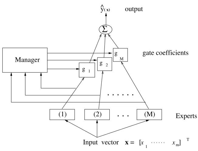
The mixture of experts network [13], as depicted in Figure 1, can be viewed as a set of linear-in-the-parameter models with convex constraints on the combination parameters through

ˆ y(x) =

M

X

j=1

gjyˆj(x) (6)

where gj ≥0,PMj=1gj = 1, ˆyj(x), j= 1,· · ·, M are the output of each expert,

and ˆy(x) is the composite output of the MEN.

Suppose thatM experts ˆyj(x) are ordered in a sequence labelled byj, j =

1,2, ..., M, and the MEN is constructed sequentially. Let a superscript (k) denote thekth forward step. At the kth forward step, the system is constructed using the firstkexperts, such that the MEN system at thekth step is

ˆ

y(k)(x) =

k

X

j=1

M

=

gate coefficients

output

x

g

Input vector

(M)

[

T

[

(2)

(1)

_Experts

^y

Manager

Σ

. . .

. . . .

g g 2 1

Fig. 1.The mixture of experts network

where g_j(k)’s are the combination coefficients at the kth step, with g(_jk) ≥ 0, Pk

j=1g (k)

j = 1, for k = 2, ..., M. The MEN system can be constructed using a

FCR procedure described below [12]:

(i) At the first step, the MEN system is the first expert.

ˆ

y(1)(x) = ˆy1(x) (8)

This means thatg(1)₁ = 1.

(ii) At the kth step, k = 2,· · ·, M, the MEN system is constructed by in-cluding thekth expert into the MEN as

ˆ

y(k)(x) =λk−1yˆ(k−1)(x) + (1−λk−1)ˆyk(x) (9)

where 0≤λk−1≤1,∀k.

It can be shown [12] that the system constructed using the FCR procedure satisfies the convex constraints condition for weights; g_j(k) ≥0,Pk

j=1g (k)

j = 1,

fork= 2, ..., M.

3.2 The Forward Constrained Regression Algorithm for Sparse Kernel Density Estimation

x6 is selected to form the first kernel, this is denoted asx01. The sparse kernel

density estimator ˆp(x;g, σ) in (5) can be regarded as a MEN system with the kernel functions K(x,x0

j) as the experts ˆyj(x). The kernel functions K(x,xj)

with nonzerogj’s are included into the model in a forward manner. At thekth

forward step, the intermediate kernel density estimator ˆp(k)(x;g(k)_{, σ) can then}

be denoted by ˆy(k)(x) as

ˆ

y(k)(x) =

k

X

j=1

g(_jk)K(x,x0j) (10)

whereg_j(k),j= 1, ..., k are the kernels weights at thekth forward step.

Initialization The initialization of the MEN system is to determine the first expert by selecting the first kernel K(x,x0

1), so that

ˆ

y(1)(x) =K(x,x0

1) (11)

andg₁(1)= 1.From (5) and (11)

ˆ

p(x;gP ar_{, σ}P ar_{) =K(x,x}0

1) +ε(x) (12)

FromN kernelsK(x,xj),j = 1, ...N, one is to be determined asK(x,x01). This

is simply done by searching for the term that produces the smallest value of mean squares modelling errors overD, i.e.

j1= arg min{

N

X

i=1

[ˆp(xi;gP ar, σP ar)−K(xi,xj)]2,∀j} (13)

andxj₁ is then set asx01.

Kernel selection using leave-one-out (LOO) test score and the jack-knife parameter estimator Now consider the model term selection for forward stepk≥2. (9) can be rewritten as

ˆ

y(k)(x) =λk−1yˆ(k−1)(x) + (1−λk−1)K(x,x0k) (14)

The right hand side of (14) is a convex combination of two terms, the current MEN system ˆy(k−1)(x) and the kth kernel K(x,x0

k) to be included into the

model at thekth forward step. The following proposed algorithm aims to resolve two problems simultaneously; (i) which kernel is to be selected asK(x,x0

k) from

(N−k+1) candidate kernels and (ii) what type of parameter estimator is adopted forλk−1.

From (5) and (14) we have

ˆ

p(x;gP ar, σP ar) =

k

X

j=1

g_j(k)K(x,x0

j) +ε(x)

WithN data samples, define ˆpP ar_{= [ˆp(x}

1;gP ar, σP ar), ...,pˆ(xN;gP ar, σP ar)]T,

ˆ

y(k−1) _{= [ˆy}(k−1)_(x

1), ...,yˆ(k−1)(xN)]T, ψ = [K(x1,x0k), ..., K(xN,x0k)]T and

ε= [ε(x1), ..., ε(xN)]T. Then (15) can be rewritten in the vector form as

ˆ

pP ar _=λ

k−1yˆ(k−1)+ (1−λk−1)ψ+ε (16)

or

t=λk−1w+ε (17)

witht= [t1, ..., tN]T = ˆpP ar−ψ,w= [w1, ..., wN]T = ˆy(k−1)−ψ.

Minimizing the loss functionJ =εTεwith respect toλk−1to yield the least

squares solution

λLS_k−1= w

T_t

wT_w

= bk−1 ak−1

(18)

wherebk−1=wTtandak−1=wTw.

The kth step of the MEN system involves the selection of K(x,x0

k). Note

that by using each of the (N−k+ 1) candidate kernels to formψin turn, (18) is repeated calculated. For some candidate kernels, the solution may not satisfy the constraints 0≤λLS_k−1 ≤1. These kernels will then not be considered to be appropriate.

For all model terms which satisfy the constraints 0≤λLS_k−1≤1, the following proposed model term selection algorithm is applied, which combines the leave-one-out cross validation with the jackknife parameter estimator forλk−1 (given

by (21) below), subject to 0≤λk−1≤1.

The leave-one-out cross validation involves the removal of each xj in turn

from the estimation data setD,j= 1, ..., N. The removed data point is used as a test point for the model constructed using the modified data set. It is easy to verify that the least squares solution using (D\xj), is given by

λ(_k−₋j₁)= bk−1−wjtj ak−1−w2j

, j= 1, ..., N (19)

and the mean squares of LOO errorsε(−j)_(x

j) is given by

Jk =E{[ε(−j)(xj)]2}=

1 N

N

X

j=1

tj−λ(k−−j1)wj

2

(20)

It is known that the jackknife parameter estimator is able to improve the accuracy of parameter estimation [14, 15]. The jackknife parameter estimator forλk−1given by

λk−1=λLSk−1−

N−1 N

N

X

j=1

is employed for parameter estimation. Although in general the jackknife param-eter estimator is regarded as computationally intensive, the additional computa-tion is minimal in the proposed algorithm. This is because in the FCR procedure, only a minimal number of one parameterλ(_k−₋j₁), (j= 1, ..., N) is involved for each candidate term. In addition, most of the calculation in parameter estimation can be regarded as the byproducts of the above leave-one-out cross validation pro-cedure.

For all model terms which satisfy the constraints 0 ≤ λLS_k−1 ≤ 1, (19)-(21) are repeatedly calculated. Amongst all solutions satisfying the constraints 0 ≤

λk−1 ≤1, the data point that produces the smallest Jk is selected asx0k and

then used to form kernelK(x,x0

k).

The parametersg(_jk)is readily computed by applying the recursion [12], given by

g_j(k)=λk−1gj(k−1), j= 1, ..., k−1

g_k(k)= 1−λk−1 (22)

withg₁(1)= 1.

The above procedure iterates for a finite number of forward steps, with k increases by one each step until the final model achieves a satisfactory modelling performance. In this work we terminate the procedure when the accuracy of the sparse kernel density estimator ˆp(x;g, σ) is sufficiently close to that of the PW density estimator ˆp(x;gP ar_{, σ}P ar_).

−8 −6 −4 −2 0 2 4 6 8

−5 0 5 0 0.01 0.02 0.03 0.04 0.05 0.06 0.07 0.08

x₁ x₂

pdf

−8 −6 −4 −2 0 2 4 6 8

−8 −6 −4 −2 0 2 4 6 8

x₁ x2

(a) (b)

−8 −6 −4 −2 0 2 4 6 8 −8

−6 −4 −2 0 2 4 6 8

x₁ x2

(a) (b)

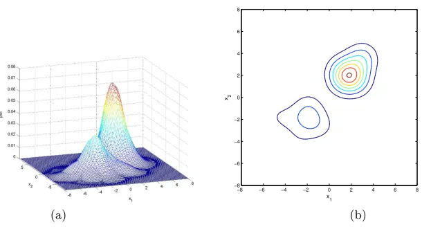
Fig. 3. (a) The Parzen window probability density estimate and (b) its contour for Example 1.

−8 −6 −4 −2 0 2 4 6 8

−8 −6 −4 −2 0 2 4 6 8

x₁ x2

(a) (b)

4

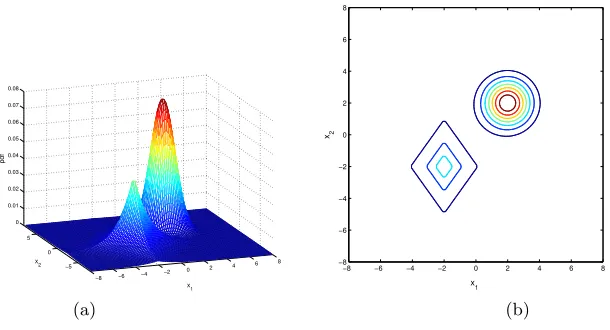
An Illustrative Example

The density to be estimated for this 2-D example was given by the mixture of two densities of a Gaussian and a Laplacian, as defined by

p(x) = 1 4πexp

−(x1−2)

2

2

exp

−(x2−2)

2

2

+0.35

8 exp(−0.7|x1+ 2|) exp(−0.5|x2+ 2|) (23)

The true density and its contour are shown in Figure 2. A data set ofN = 500 points was randomly drawn from this distribution and used to construct the probability density function ˆp(x;g, σ) using the proposed FCR-SDC approach. The kernel width of σP ar = 0.4 was empirically found and used in the Parzen window estimate initially, and then the kernel width of σ= 1 was used in the FCR-SDC algorithm. A separate test data set ofNtest = 10000 points was used

for evaluation according to

L1=

1 Ntest

Ntest

X

k=1

|p(xk)−pˆ(xk;g, σ)| (24)

The experiment was repeated for 100 different random runs. The results of the proposed method in comparison with the PW estimate and the SDC [10] are shown in Table 1. It is shown that the proposed FCR-SDC has comparable accuracy to that of PW, with an average number of required kernels less that 6% of the data samples. In term of model sparsity and accuracy the best performance is that of SDC [10]. The typical Parzen window estimate and the FCR-SDC estimate were depicted in Figures 3–4.

Table 1.Performance of the three kernel density estimates for Example 1.

Method L1 test error (mean±STD) Kernel numbers (mean±STD)

PW (4.20±_0.8)×₁₀−3 ₅₀₀±₀

SDC [10] (3.63±_0.8)×₁₀−3 _11.9±_2.6

proposed FCR-SDC (4.26±_0.7)×₁₀−3 _33.6±_4.7

5

Conclusions

proposed algorithm are able to model the probability density function with com-parable accuracy, but with a much sparser representation than Parzen window estimate. Hence the proposed algorithm offers as a viable alternative for sparse probability density function estimation.

References

1. Silverman, B. W.: Density Estimation for Statistics and Data Analysis, Chapman and Hall (1986)

2. Duda, R. O., Hart, P. E.: Pattern Classification and Scene Analysis, J. Wiley (1973) 3. Bishop, C. M.: Neural Networks for Pattern Recognition, Oxford University Press

(1995)

4. Parzen, E.: On estimation of a probability density function and mode, The Annals of Mathematical Statistics33(1962) 1065–1076

5. McLachlan, G., Peel, D.: Finite Mixture Models, J. Wiley (2000)

6. Weston,J., Gammerman, A., Stitson,M.O., Vapnik,V., Vovk,v. , Watkins,C.: Sup-pot vector density estimation, in Burges C., Sch¨olkopf B., Smola, A. J.(eds) Ad-vances in Kernel Methods, MIT Press (1999) 293–306.

7. Vapnik, V., Mukherjee,S.: Support vector machine for multivariate density esti-mation, in Leen, T., Solla, S.,M¨uller, K. R.(eds) Advances in Neural Infromation Processing Systems. MIT Press (2000) 659–665

8. Girolami, M., He, C.: Probability density estimation from optimally condensed data samples, IEEE Trans. on Pattern Analysis and Machine Intelligence25(2003) 1253–1264

9. Choudhury, A.: Fast Machine Learning Algorithms for Large Data, Ph.D. thesis, School of Engineering Sciences, University of Southampton, UK (2002)

10. Chen, S., Hong, X., Harris, C. J.: Sparse kernel density construction using orthogo-nal forward regression with leave-one-out test score and local regularization, IEEE Trans. on Systems, Man and Cybernetics, Part B34(2004) 1708–1717

11. Chen, S., Hong, X., Harris, C. J.: An orthogonal forward regression technique for sparse kernel density estimation, Neurocomputing (2007) To appear

12. Hong, X., Harris, C. J: A mixture of experts network structure construction algo-rithm for modelling and control, Applied Intelligence16(2002) 59–69

13. Jordan, M., Jacobs, R. A.: Hierarchical mixtures of experts and the EM algorithm, Neural Computation6(1994) 181–214