On the linear quadratic data-driven control
Ivan Markovsky and Paolo Rapisarda
School of Electronics and Computer Science, University of Southampton
Southampton, SO17 1BJ, United Kingdom
{im,pr3}@ecs.soton.ac.uk
Abstract— The classical approach for solving control prob-lems is model based: first a model representation is derived from given data of the plant and then a control law is synthesized using the model and the control specifications. We present an alternative approach that circumvents the explicit identification of a model representation. The considered control problem is finite horizon linear quadratic tracking. The results are derived assuming exact data and the optimal trajectory is constructed off-line.
I. INTRODUCTION
We consider a finite horizon linear quadratic tracking problem that takes as input data a trajectory of the to-be-controlled plant instead of an input/state/output representa-tion. Such a formulation is considered to be closer to a real-life control problem, because in practice one rarely has an input/state/output representation but often has measurements (i.e., an observed trajectory) of the plant. In addition, as shown in this paper, our formulation gives more freedom in the choice of the approach for solving the problem.
The classical approach for solving the control problem is model based. First, a plant model is explicitly identified from the data and, second, a controller that achieves the desired specifications is synthesized using the model. Thus, the control problem is split into two independent stages:
1) identification and 2) model-based synthesis.
The control objectives are not taken into account in the identification part and once the model is computed from the data, the data is not used in the synthesis of the controller. Both system identification and controller synthesis are ma-ture research areas, however, their interplay in solving the overall problem from data to control has only recently been addressed in a new field, called identification for control.
Identification for control aims to determine the “best” model to be used with a given model-based synthesis method. Presently, there are only partial results in solving this prob-lem. In its full generality, the question what is the best model for control seems to be as hard as the original problem that aims to derive optimal control directly from the available data.
An alternative to the model based paradigm is the deriva-tion of the optimal control input or the optimal controller directly from the data. This paradigm has also been explored in the literature. Different authors call it with different names: data-based, data-driven, unfalsified [1], [2], model-free [3],
[4], and model-less control. In this paper, we refer to the direct construction of the control from data as data-driven control.
Perhaps the first data-driven control method is the Ziegler-Nichols procedure for tuning PID controllers. It is based, however, on the plant step response, which is a very special response. In addition, the method is graphical and does not generalize to other control problems. A procedure for deriving multivariable linear quadratic Gaussian controller, using the plant impulse response, is proposed in [5]. Data-driven synthesis methods using an arbitrary response are proposed in [6] (linear quadratic regulation) and [7], [8] (linear quadratic tracking).
In this paper we consider a data-driven finite horizon linear quadratic tracking problem, where the given trajectorywdis assumed to be exact and the plant B is assumed to be a linear time-invariant system. (The more realistic but harder to deal with situation when the data is perturbed will be treated elsewhere.) In Section II, we present three solutions for this problem. The first one is the classical model-based control that first computes an input/state/output representation of the plant and then synthesizes the controller by solving the corresponding Riccati equation. The second approach computes an impulse response representation of the plant and then finds the optimal trajectory by solving a weighted least squares problem. These approaches derive explicitly a representation of the plant. The third approach computes the optimal trajectory directly from the given data without computing a representation of the plant. The idea is to project the reference trajectory on the subbehaviorB0of the plant, consisting of all zero initial conditions trajectories. Under certain specified conditions,B0 can be computed fromwd, which makes the procedure implementable.
Preliminaries and notation
We use the behavioral language. A discrete-time dy-namical system B is a subset of the signal space (Rw)N.
The integer w is the number of variables and the set of natural numbers N is the time axis. We consider linear,
time-invariant, and finite dimensional systems, so that B is a closed shift-invariant subspace of (Rw)N. In addition,
we assume that a trajectory w of B has an input/output partition col(u,y). (In general one needs to permute the
variables in order to have the inputs as the first variables.) B|[
t1,t2]denotes the restriction of the behavior on the interval
[t1,t2], i.e.,
B|[t
1,t2]:={w∈(
Rw)t2−t1 | there are wpandwf, such that col(wp,w,wf)∈B}.
σ denotes the backwards shift operatorσw(t) =w(t+1). The Hankel matrix with t block rows, composed of the sequencew∈(Rw)T is denoted by
Ht
1,t2(w):=
w(1) w(2) · · · w(t2) w(2) w(3) · · · w(t2+1) w(3) w(4) · · · w(t2+2)
. . .
. . .
. . .
w(t1) w(t1+1) · · · w(t1+t2−1)
. (1)
If the index t2 is skipped, it is assumed to have the maxi-mal possible value T−t1+1. The lower-triangular Toeplitz matrix with t block rows, composed of the sequence h=
h(0),h(1), . . . ,h(t−1)
is denoted by
Tt(h):=
h(0)
h(1) h(0) h(2) h(1) h(0)
. . .
. .
. .
. .
. .
.
h(t−1) · · · h(1) h(0)
. (2)
The integer n(B) is the order ofB andl(B)is the lag of B (i.e., the observability index of B). Throughout the paper,m denotes the number of inputs andp the number of output ofB.
The time series u= u(1), . . . ,u(T)
is persistently excit-ing of orderLif the Hankel matrixHL(u)is of full row rank. “rowdim” denotes the number ofblock rows of a matrix or vector, andA+denotes the Moore-Penrose pseudoinverse of the matrixA.
II. LINEAR QUADRATIC TRACKING
In a linear quadratic tracking problem the objective is to choose the control inputs in such a way that the plant B follows as close as possible in the sense of the quadratic error criterion
J(wr,w):= Tr
∑
t=1wr(t)−w(t)⊤Φ wr(t)−w(t)
, (3)
a given reference trajectorywr∈(Rw)Tr. In the definition of
the criterionJ,Φ∈Rw×wis a positive definite weight matrix andTr is the tracking horizon.
In the special case when the reference trajectory is the zero trajectory, the tracking problem becomes the regulation problem. In this case, the optimal tracking, aiming solely at minimizing the criterion J(wr,·) over all trajectories of B,
has a trivial solution—the zero trajectory. The regulation problem is meaningful, when a nonzero initial condition is specified for the plantB. Therefore, we will introduce initial conditions specification in the general tracking problem.
In a representation free setting, we specify initial condition by requiring the system to follow a given initial trajec-torywini∈(Rw)Tini. Ifwini∈Bisl(B)or more samples long, following wini, the system has a uniquely determined final state. This final state serves as an initial conditionxinifor the tracking problem. (See (4) and (5), where the minimality of the state representation andTini≥l(B)ensure that the system of equations for the initial statex(1)has a unique solution, which determines a unique final statex(Tini+1) =:xini.)
The classical formulation of the tracking problem starts with a given input/state/output representation of the sys-tem B. In the context of data-driven tracking, we start instead from a given trajectory wd∈(Rw)T of B, which
under the conditions of [11], uniquely specifies B. In the solution of the data-driven tracking problem, we aim at finding the optimal trajectory without explicitly computing a representation (in particular an input/state/output representa-tion) ofB.
Problem 1(Linear quadratic tracking). Given 1) a trajectorywd= wd(1), . . . ,wd(T)
of a linear time-invariant systemB,
2) a reference trajectorywr= wr(1), . . . ,wr(Tr)
, 3) an initial trajectorywini= wini(1), . . . ,wini(Tini)
∈B, 4) a positive definite matrixΦ∈Rw×w,
find a trajectory of B that is optimal with respect to the performance criterion J(wr,·) (see (3)) and has as a prefix
the initial trajectorywini, i.e., solve the problem min
wf J(wr
,wf) subject to col(wini,wf)∈B.
A. Solution using an input/state/output representation The classical but indirect solution of Problem 1 is to compute first a state space representation
σx=Ax+Bu, y=Cx+Du
ofBfrom the datawdand then using(A,B,C,D)to compute
the optimal trajectory w∗f. This is the well known model-based approach that we summarize for completeness.
By assumption the data wd is an exact trajectory of the unknown systemB. Therefore, we are dealing with an exact (deterministic) identification problem wd7→B. Sufficient conditions for identifiability are (see [11]):
1) Bis controllable,
2) ud is persistently exciting of ordern(B) +l(B) +1, i.e.,H
n(B)+l(B)+1(ud)is full rank.
Once the parameters (A,B,C,D) of a minimal
in-put/state/output representation of B are available we can find the initial condition xini for the tracking problem that is induced by the initial trajectory wini. This is an observer design problem. Let col(yini,uini) be an input/output
parti-tioning ofwini and leth be the impulse response ofB, i.e.,
h(0) =D, h(t) =CA
t−1B
, fort=1,2, . . . .
Then
yini=
C CA
. . .
CATini−1
x(1) +TTini(h)uini (4)
defines a system of equations for the initial statex(1). This system has a unique solution since by assumptionwiniis an exact trajectory ofB(existence) and(A
,B,C,D)is a minimal
representation (uniqueness). The initial conditionxinifor the tracking problem is equal to the final statex(Tini+1)ofB, followingwini, i.e.,
xini=x(Tini+1) =CATinix(1)+
h(Tini−1) h(Tini−2) · · · h(0)
uini. (5)
Once the state space representation and the initial state are available, Problem 1 becomes
min
x,u,y
Tr
∑
t=1wr(t)−
u(t) y(t)
⊤
Φ
wr(t)−
u(t) y(t)
subject to x(t+1) =Ax(t) +Bu(t), x(1) =xini
y(t) =Cx(t) +Du(t), fort=1, . . . ,Tr.
(6)
The solution leads to a difference Riccati equation that depends only on the A,B,C,D matrices and a backward in
time recursion that depends on the reference signal wr and the initial condition xini. The formulas for the continuous-time case are given in [13, Theorem 1]. We were not able, however, to find in the literature the solution for the discrete-time tracking problem (6), so we give next the solution for the finite-horizon linear quadratic regulation, i.e., for the special case ofwr=0.
We can eliminate the variableyin (6) by substitution. This gives the following linear quadratic regulation problem with complete state information
min
x,u
Tr
∑
t=1u(t) x(t)
⊤
I 0
D C
⊤
Φ
I 0
D C
u(t) x(t)
subject to x(t+1) =Ax(t) +Bu(t), x(1) =xini
fort=1, . . . ,Tr.
(7)
Define the partitioning
Φ=:
Φ
u Φuy
Φyu Φy
.
The solution of (7) is (see, e.g., [14, Theorem 11.1])
x∗(t+1) = (A−BLt)x∗(t), x(1) =xini,
w∗f(t) =
−Lt
C−DLt
x∗(t),
(8)
where
Lt:= B⊤St+1B+Φu+ΦuyD+D⊤Φ⊤uy+D⊤ΦyD−1
× B⊤St+1A+ΦuyC+D⊤ΦyC (9) and
St=A⊤St+1A+C⊤ΦyC− B⊤St+1A+ΦuyC+D⊤ΦyC⊤
× B⊤St+1B+Φu+ΦuyD+D⊤Φ⊤uy+D⊤ΦyD−1 × B⊤St+1A+ΦuyC+D⊤ΦyC, STr=0. (10)
In summary, an algorithm for solving Problem 1, in the special case wr = 0, using an input/state/output representation of the plant is:
1) wd−−−−−−−−−−−−−−−−−−→Identification [10, Algorithm 8.5] (A,B,C,D)
2) (wini,A,B,C,D)
Observer (4) and (5) −−−−−−−−−−−→xini
3) (Φ,wr,xini,A,B,C,D)
Synthesis (8,9,10) −−−−−−−−−→w∗f
Note 2. Algorithm 8.5 of [10] needs, in addition to the data wd, an upper bound lmax for the system lag l(B). The same is true for Algorithms 8.7 and 8.9 of [10] and Algorithm 2 of [15], which are referred to later in this paper. Although we do not write it explicitly, we do assume that such an upper bound is given as part of the problem formulation and is passed to the identification algorithms.
B. Solution using an impulse response representation Another approach is to compute the impulse response h of B from the data wd and then using h to compute w∗. Condition (A) is sufficient for being able to derivehfromwd, see [10, Section 8.6]. Moreover, there are algorithms for doing this. Although this approach does not derive the classical input/state/output representation of the system B for computing w∗, it is not data driven either (the impulse response is a representation ofB).
Let the columns ofO ben(B)linearly independent zero-input trajectories ofB. (Such a matrix can also be computed from data, see [10, Section 8.8].) Any zero-input trajectory ofB can be written asOxini, for somexini∈Rn. Define
˜
h(0) =col Im,h(0)
, and
˜
h(t) =col 0m,h(t)
, fort=1,2, . . . ,
where Im is the m×m identity matrix and 0m is the m×m zero matrix. Then for any trajectory
w:=col(wini,wf)∈B|[1
,Tini+Tr]
there is a corresponding initial condition xini and an input sequence col(uini,uf), such that
wini
wf
=Ox(1) +TT
ini+Tr(h˜)
uini
uf
. (11)
(See (2) for the definition ofT.) Define the partitionings O
1 O2
and TT
ini+Tr(h˜) =
T11 0
T21 TTr(h˜)
that are conformable with the partitionings of col(wini,wf)
and col(uini,uf). The equations in (11) with
left-hand-sidewini
wini=O1x(1) +T11uini (12)
are decoupled from the other equations and can be solved independently in terms of the initial state x(1) and initial input sequenceuini. The remaining equations
wf=O2x(1) +T21uini+TTr(h˜)uf
specifywf in terms of the inputuf. Define
wf,1:=
O2x(1) +T21uini. (13)
Note thatwf,1is the free response of
B, caused by the initial trajectory wini (or equivalently by the initial conditionxini), i.e., it is of the formwf,1=col(0,yf,1).
The optimal tracking problem becomes
min
uf J wr ,wf,1+
TTr(h˜)uf
,
which is a standard weighted least squares problem. Its solution is
u∗f= T⊤
Tr (h˜)Φ˜TTr(h˜)
−1T⊤
Tr (h˜)Φ˜(wr−wf,1), (14)
where ˜Φ=diag(Φ, . . . ,Φ)∈RTrw×Trw, so that
w∗f =TTr(h˜)u∗f+wf,1. (15)
In summary, an algorithm for solving Problem 1, using an impulse response representation of the plant is:
1) (wd,Tr)
[10, Algorithms 8.7 and 8.9] −−−−−−−−−−−−−−−→(h,O)
2) (wini,h,O) (12,13) −−−−→wf,1
3) (Φ,wr,wf,1,h)
(14,15) −−−−→w∗f
C. Data-driven solution
A third possibility, which gives a truly data-driven solu-tion, is to project the trajectorywr−wf,1 on the zero initial
conditions subbehavior ofB:
B0|[1
,Tr]:=
w∈(Rw)Tr | col(0
l(B)w×1,w)∈B|[1
,l(B)+Tr] .
The definition says thatB0consists of all trajectories ofB that when extended withl(B)zero samples are still trajecto-ries ofB. Thel(B)trailing zero samples specify zero initial conditions, soB0is indeed the subspace ofBconsisting of all zero initial conditions trajectories.
Theorem 3. Let W0∈RTrwו be a matrix, such that
image W0
=B0|[1
,Tr].
Then the solution of Problem 1 is given by
w∗f =W0 W0⊤Φ˜W0
+
W0⊤Φ˜(wr−wf,1) +wf,1, (16)
where wf,1 is the free response of
B, caused by the initial
trajectory winiand(·)+is the Moore-Penrose pseudoinverse.
If W0 defines a basis for B0|[1
,Tr], then the pseudoinverse
in (16) can be replaced by inverse.
Proof: Any zero initial conditions trajectory w=
col(u,y)∈(R
w)Tr is of the form w=T
Tr(h˜)u. Therefore,
B0|[1
,Tr]=image
TTr(h˜)
=image W0.
Consider the spaceW = (Rw)Tr with inner product defined
byhw1,w2i=w
⊤
1Φ˜w2. The projector onB0|[1,Tr] in
W is
TTr(h˜) T⊤
Tr(h˜)Φ˜TTr(h˜)−1TTr⊤(h˜)Φ˜
=W0 W0⊤Φ˜W0+W0⊤Φ.˜
Then (16) follows from (14,15).
Theorem 3 is based on the fact that the optimal solution w∗f depends only on the subspaceB0|[1
,Tr], the metric, given
by the weight matrixΦ, and the free responsewf,1, initiated
bywini, and not on the particular basis ofB0|[1,Tr]. In (14,15),
we used as a basis forB0|[1
,Tr] the columns of the Toeplitz
matrixTTr(h˜)constructed from the impulse response ofB. Suppose, however, that we are able to find from the given datawdanother basisW0forB0. Then the optimal trajectory would be given by (16). In addition, the free response wf,1
can be computed directly from the datawd, using the data driven simulation algorithm of [15], so we would completely circumvent the need to compute the impulse responseh. A procedure for construction of a matrixW0 which columns spanB0is given in the next section.
In summary, a data-driven algorithm for solving Problem 1 is:
1) (wd,Tr)
Section III, Algorithm 1 −−−−−−−−−−−−−→W0 2) (wini,wd,Tr)
[15, Algorithm 2] −−−−−−−−−→wf,1
3) (Φ,wr,wf,1,W0)
(16) −−→w∗f
III. COMPUTATION OF A BASIS FORB0 Under the assumptions of Theorem 1 from [11]: 1) B controllable,
2) wd∈B|[1,T], and
3) udpersistently exciting of order lmax+Tr+n(B)), we have that
image Hl
max+Tr(wd)
=B|[1
,lmax+Tr].
(See (1) for the definition ofH.) Therefore, anylmax+Tr -samples long trajectory ofBcan be constructed as a linear combination of the columns ofHl
max+Tr(wd),
w∈B|[1
,lmax+Tr] ⇐⇒ there isg∈
RT−lmax−Tr+1
such thatw=Hl
max+Tr(wd)g. (17)
Assuming that lmax ≥l(B), see Note 2, the first lmax samples of w (referred to as the “past”) can be used to set up initial conditions for the remaining response (referred to as the “future”). From (17) and the definition of B0|[1
,Tr] it
follows that
w∈B0|[1
,Tr] ⇐⇒ there isg∈
RT−lmax−Tr+1,
Next we introduce some notation. Define the Hankel matrices from the input and the output
U:=Hl
max+Tr(ud), Y :=Hlmax+Tr(yd)
and their past/future partitionings
U=:
Up Uf
, Y =:
Yp Yf
,
where rowdim(Up) =rowdim(Yp) =lmaxand rowdim(Uf) = rowdim(Yf) =Tr. Permuting the equations of the system
Hlmax+Tr(wd)g=col(0lmaxw×1,w)
we have the equivalent system
Up Yp Uf Yf
g=
0lmaxm×1 0lmaxp×1
u y
.
Given an arbitrary input vector u, we can compute the corresponding output vector y, such that col(u,y)∈B0 as
follows:
1) solve the system of equations forg
Up Yp Uf
g=
0lmaxm×1 0lmaxp×1
u
2) definey=Yfg.
This gives us a procedure for computing an element ofB0. In order to compute a set of generators for B0|[1
,Tr],
we need to compute at least dim(B0|[1
,Tr]) =Trm linearly
independent elements of B0|[1
,Tr]. This can be done as
outlined in Algorithm 1.
Algorithm 1 Block computation of a basis forB0|[1
,Tr]
Input: ud,yd,lmax, andTr.
1: Solve the system of equations for G
Up
Yp Uf
G=
0lmaxm×Trm 0lmaxp×Trm HTr
,Trm(ud)
.
2: ComputeY0=YfG.
Output: a basis col HTr
,Trm(ud),Y0
for B 0|[1,Tr].
Due to the persistency of excitation of ud, the Han-kel matrix HTr
,Trm(ud) is full rank and the computed
responses, given by the columns of col HTr
,Trm(ud),Y0
, are linearly independent. Therefore, a desired matrix W0, such that image(W0) = B0|[1,Tr], can be obtained from
col HTr
,Trm(ud),Y0
by permutation of the rows.
Note 4. Algorithm 1 corresponds to the block algorithm of [9] for the computation of the impulse response. It requires persistency of excitation of order lmax+Tr+n(B) for ud. A recursive version of Algorithm 1, derived along the lines of the recursive algorithm of [9] for the computation of the impulse response, however, requires persistency of excitation for ud of order lmax+n(B) +1. Note that this is the same condition that is required for identifiability of B.
IV. SIMULATION EXAMPLES
The aim of the simulation examples, shown in this section, is to illustrate numerically the equivalence of the three methods for data-driven control, presented in the paper. The to-be-controlled plantBis a linear time-invariant system of ordern=2, withm=1 input andp=1 output. It is induced by the transfer function
¯
H(z) =(z−0.7847)(z+1.17)
z2−1.615z+0.6972 .
The datawd, used by the algorithms, is a random trajectory ofBwithT=200 samples. It is the same in all simulations. A reference trajectory wr with Tr samples and an initial trajectory wini with Tini=l(B) =2 samples are chosen as follows:
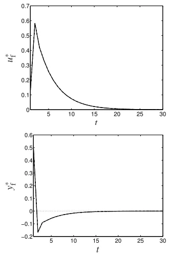
• Experiment 1: data-driven regulationTr=30 wr=0 and wini= (1,1),
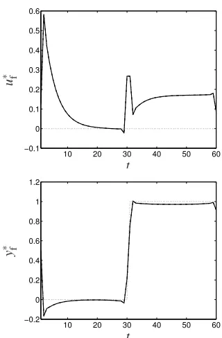
• Experiment 2: data-driven step trackingTr=60
ur=0, yr(t) =
(
0, fort=1,2. . . ,30,
1, fort=31,52, . . . ,60,
andwini= (1,1).
In both experiments,Φ is the 2×2 identity matrix.
In the first experiment the three methods compute the same optimal trajectory, see Figure 1. The corresponding optimal value of the cost functional is J(0,w
∗
f) =1.1139.
5 10 15 20 25 30
0 0.1 0.2 0.3 0.4 0.5 0.6 0.7
t
u
∗ f
5 10 15 20 25 30
−0.2 −0.1 0 0.1 0.2 0.3 0.4 0.5 0.6
t
y
∗ f
Fig. 1. First experiment:wrdotted line,w∗f solid line.
In the second experiment, we compare only the second and the third approach. (We do not have the solution of the general tracking problem by the input/state/output approach.) The two solutions coincide and are shown on Figure 2. The corresponding optimal value of the cost functional is J(wr,w
∗
[image:5.612.348.513.391.639.2]10 20 30 40 50 60 −0.1
0 0.1 0.2 0.3 0.4 0.5 0.6
t
u
∗ f
10 20 30 40 50 60
−0.2 0 0.2 0.4 0.6 0.8 1 1.2
t
y
∗ f
Fig. 2. Second experiment:wrdotted line,w∗f solid line.
V. CONCLUSIONS
We considered a finite horizon linear quadratic tracking problem, where the given data is assumed exact, and pre-sented three solutions to the problem. All solutions need the same basic assumptions: 1) the plantBis controllable, and 2) an input component of the given trajectory is persistently exciting of order n(B) +l(B) +1. The solution given by the input/state/outout approach, however, is in the form of a feedback, while the other solutions compute off-line the optimal trajectory. In [5] a procedure for computing the optimal controller from the impulse response of the plant is described, however, the question “How to compute the optimal controller directly from data?” is yet unsolved.
Another important issue that we did not discuss is “How to compute the optimal trajectory or the optimal controller recursively?” In [9] a procedure for recursive computation of the impulse response is presented. Combined with recursive least squares for computing the optimal trajectory, given by (16), we obtain a recursive algorithm. Recursive imple-mentation of the algorithm, however, does not necessarily imply suitability for on-line implementation. The algorithm should in addition be causal, i.e., operating in real time it should use only past data.
Apart from the on-line implementation, another important issue is to adapt the methods, to “work well” with perturbed data. In this paper a restrictive assumption is that the given trajectory of the plant is exact and the plant is a low-order linear time-invariant system. In practice, the data is noisy and the plant is likely to be nonlinear and time-varying. This makes it necessary to modify the algorithms in order to allow for approximation. The final goal of this work is to obtain approximate recursive algorithms for data-driven control.
ACKNOWLEDGMENTS
Research supported by:Research Council KUL:GOA-Mefisto
666, GOA-Ambiorics, IDO/99/003 and IDO/02/009 (Predictive computer models for medical classification problems using pa-tient data and expert knowledge), several PhD/postdoc & fellow
grants;Flemish Government: FWO:PhD/postdoc grants, projects,
G.0078.01 (structured matrices), G.0269.02 (magnetic resonance spectroscopic imaging), G.0270.02 (nonlinear Lp approximation), G.0240.99 (multilinear algebra), G.0407.02 (support vector ma-chines), G.0197.02 (power islands), G.0141.03 (Identification and cryptography), G.0491.03 (control for intensive care glycemia), G.0120.03 (QIT), G.0452.04 (QC), G.0499.04 (robust SVM), re-search communities (ICCoS, ANMMM, MLDM); AWI: Bil. Int.
Collaboration Hungary/ Poland; IWT: PhD Grants; GBOU
(Mc-Know)Belgian Federal Government:DWTC (IUAP IV-02
(1996-2001) and Belgian Federal Science Policy Office IUAP V-22 (2002-2006) (Dynamical Systems and Control: Computation, Identifica-tion & Modelling)); PODO-II (CP/01/40: TMS and
Sustainibil-ity);EU: PDT-COIL, BIOPATTERN, eTUMOUR, FP5-Quprodis;
ERNSI; Eureka 2063-IMPACT; Eureka 2419-FliTE; Contract Re-search/agreements: ISMC/IPCOS, Data4s, TML, Elia, LMS, IP-COS, Mastercard. and the University of Southampton
REFERENCES
[1] M. Safonov, “Focusing on the knowable: Controller invalidation and learning,” in Control using logic-based switching, A. Morse, Ed. Springer-Verlag, Berlin, 1996, pp. 224–233.
[2] M. Safonov and T. Tsao, “The unfalsified control concept and learn-ing,”IEEE Trans. Automat. Control, vol. 42, no. 6, pp. 843–847, 1997. [3] W. Favoreel, “Subspace metods for identification and control of linear and bilinear systems,” Ph.D. dissertation, Faculty of Engineering, K.U.Leuven, 1999.
[4] B. Woodley, “Model free subspace based H∞control,” Ph.D.
disserta-tion, Stanford University, 2001.
[5] K. Furuta and M. Wongsaisuwan, “Discrete-time LQG dynamic con-troller design using plant Markov parameters,” Automatica, vol. 31, no. 9, pp. 1317–1324, 1995.
[6] J.-T. Chan, “Data-based synthesis of a multivariable linear-quadratic regulator,”Automatica, vol. 32, pp. 403–407, 1996.
[7] M. Ikeda, Y. Fujisaki, and N. Hayashi, “A model-less algorithm for tracking control based on input-ouput data,” Nonlinear alalysis, vol. 47, pp. 1953–1960, 2001.
[8] Y. Fujisaki, Y. Duan, and M. Ikeda, “System representation and optimal control in input-output data space,” in Proc. 10th IFAC Symposium on Large Scale Systems, Osaka, Japan, 2004, pp. 197– 202.
[9] I. Markovsky, J. C. Willems, P. Rapisarda, and B. D. Moor, “Algo-rithms for deterministic balanced subspace identification,”Automatica, vol. 41, no. 5, pp. 755–766, 2005.
[10] I. Markovsky, J. C. Willems, S. Van Huffel, and B. De Moor,Exact and Approximate Modeling of Linear Systems: A Behavioral Approach, ser. Monographs on Mathematical Modeling and Computation. SIAM, March 2006, no. 11.
[11] J. C. Willems, P. Rapisarda, I. Markovsky, and B. D. Moor, “A note on persistency of excitation,”Control Lett., vol. 54, no. 4, pp. 325–329, 2005.
[12] P. Van Overschee and B. De Moor,Subspace Identification for Linear Systems: Theory, Implementation, Applications. Boston: Kluwer, 1996.
[13] I. Markovsky, J. C. Willems, and B. De Moor, “Continuous-time errors-in-variables filtering,” in Proceedings of the 41st Conference on Decision and Control, Las Vegas, NV, 2002, pp. 2576–2581. [14] K. Åström and B. Wittenmark,Computer Control Systems: Theory
and Design. Prentice Hall, 1997.
[image:6.612.92.252.57.301.2]