An adaptive mesh refinement method for solution of the transported PDF equation

This is a repository copy of

An adaptive mesh refinement method for solution of the

transported PDF equation

.

White Rose Research Online URL for this paper:

http://eprints.whiterose.ac.uk/85259/

Version: Accepted Version

Article:

Olivieri, D, Fairweather, M and Falle, S (2009) An adaptive mesh refinement method for

solution of the transported PDF equation. International Journal for Numerical Methods in

Engineering, 79 (12). pp. 1536-1556. ISSN 0029-5981

https://doi.org/10.1002/nme.2628

© 2009 John Wiley & Sons, Ltd. This is an author produced version of a paper published in

International Journal for Numerical Methods in Engineering. Uploaded in accordance with

the publisher's self-archiving policy.

[email protected] https://eprints.whiterose.ac.uk/

Reuse

Items deposited in White Rose Research Online are protected by copyright, with all rights reserved unless indicated otherwise. They may be downloaded and/or printed for private study, or other acts as permitted by national copyright laws. The publisher or other rights holders may allow further reproduction and re-use of the full text version. This is indicated by the licence information on the White Rose Research Online record for the item.

Takedown

If you consider content in White Rose Research Online to be in breach of UK law, please notify us by

An Adaptive Mesh Refinement Method for Solution

of the Transported PDF Equation

D.A. Olivieri

_{, M. Fairweather}

_{and S.A.E.G. Falle}

1

School of Process, Environmental and Materials Engineering, The University of Leeds, Leeds LS2 9JT, U.K.

2

School of Mathematics, The University of Leeds, Leeds LS2 9JT, U.K.

*

[email protected]

Summary

This paper presents the results of an investigation into a possible alternative to Monte Carlo methods for solving the transported probability density function (PDF) equation for scalars (compositions). The method uses a finite-volume approach combined with adaptive mesh refinement (AMR) in a multidimensional compositional space. Comparisons are made between the new method and Monte Carlo solutions for analytical test cases involving the reaction of two or three chemical species. These tests demonstrate the potential of the new method in terms of both accuracy and run time. Additional test cases involving various models for molecular mixing were also conducted with similar conclusions.

Keywords: transported PDF; adaptive mesh refinement; finite-volume method; Eulerian Monte Carlo; molecular mixing

1. Introduction

Turbulent fluid flow is pervasive and there is no doubt about its importance in engineering systems. However, the reliable prediction of turbulent flows in practical situations using engineering models remains an elusive goal. Direct numerical simulation is possible, but only well below the high Reynolds numbers that arise in most applications. It is possible to use large eddy simulation (LES) at such Reynolds numbers, but computer run times restrict its use for practical engineering systems. Reynolds-averaged Navier-Stokes (RANS) techniques will therefore remain the principal method for simulating the effects of turbulence in engineering applications, despite the fact that techniques such as LES do offer benefits when time accurate results are required [1]. In RANS approaches, the Reynolds decomposition is used to derive equations for the mean values of the flow variables from the Navier-Stokes equations. Since these equations contain terms that involve the unknown fluctuating parts of the variables, they have to be supplemented by some sort of closure model.

In current RANS approaches this most frequently means the adoption of eddy viscosity or second-moment turbulence closures to model the unknown terms. However, despite their success in predicting many practical flows, these models are still dependent on the use of experimental data and generally require modifications for different types of flow. Nevertheless, these methods are still the most useful ones available for modelling turbulent flow.

The unknown terms in the equations for the mean values involve averages of various moments of the fluctuating variables, with most current RANS models using only the first two moments. Since it is generally assumed that the fluctuating part of the flow variables is described by a probability density function (PDF), it makes sense to try to determine the unknown terms from this PDF. This has the advantage that convection is represented exactly without modelling assumptions and the statistical information contained in the PDF provides a more full description of a turbulent flow than is available from a few moments. In addition, for chemically reacting flows, the terms for chemical source production in composition space appearing in the PDF equation are closed and known.

the computational cost becomes prohibitive as the number of variables increases; Pope [2] estimated that the cost increases exponentially with the number of variables. In contrast, it is claimed [2] that for Monte Carlo methods, in which the PDF is simulated using an ensemble of stochastic particles, the computational cost only increases linearly with the number of variables. It is for this reason that all current PDF transport equation solution methods are based upon Monte Carlo techniques. Janicka et al. [4] modelled the PDF equation using a finite-volume technique and were able to confirm Pope’s estimates of the computational cost. However, Sabel’nikov and Soulard [5] carried out a detailed review of all current Monte Carlo methods used in practical turbulent flow models and also compared these with the finite-volume methods. They found that the computational cost increases exponentially with the number of species for both Monte Carlo and finite-volume methods if one insists on preserving the same level of accuracy as the number of species increases.

Monte Carlo techniques are in some sense naturally adaptive, since the particles are concentrated in those parts of compositional space in which the PDF differs significantly from zero. This is not true of finite-volume methods on a uniform grid, but this limitation can be overcome by the use of AMR in which the grid can be locally refined based upon some error tolerance. This can certainly ensure that the computational effort is concentrated, where the PDF differs significantly from zero, but it is much more flexible than Monte Carlo. In particular, it will use a fine grid even in regions where the PDF is small if the error estimator says that this is necessary.

In the last two decades there has been a tremendous increase in the use of AMR, with the focus being mainly on hyperbolic systems such as compressible flow [6-8]. This is simply because such flows involve thin regions such as shocks and slip lines that require much higher resolution than the bulk of the flow. These methods have also been implemented on parallel machines using message passing (e.g. [9-13]).

All these applications concern the use of AMR in physical space, but the same ideas can be used for the PDF transport equation in both physical and compositional space. The advantage of this is that the resolution is concentrated in those areas of both physical and compositional space where it is needed. As we shall see, the method is particularly efficient when the PDF is close to a delta-function. In this paper we consider the use of a finite-volume method combined with such an AMR technique as an alternative to the use of Monte Carlo. Since our purpose is to compare both the accuracy and efficiency of the two methods, we confine ourselves to simple but generic problems, for which we can either obtain an analytic solution or use sufficient resolution to ensure numerical convergence.

2. Numerical Method

2.1. Model PDF equation

In order to demonstrate the effectiveness of the proposed method, we consider a simple joint scalar PDF equation that represents a reacting system with no spatial dependence. Despite its simplicity, this equation captures the essential features of the full equation as described in [2, 14].

Consider a reacting system of Nspecies with concentrations (= 1... N)that satisfy the reaction

equations

whereSis the rate of the chemical reaction for specie of a particular concentration. A model

PDF equation that governs the evolution of the probability P(1 ... 2; t) of a particular set of  at

timetis then

2.2. Upwind finite-volume method

Since the  are known, Equation (2) is simply a multi-dimensional linear advection equation for P,

and can be solved using an upwind finite-volume method. If the PDF were guaranteed to be smooth, then one could use a high-order advection scheme, but, as we shall see, it can often be close to a delta-function. We will therefore use a scheme that has been developed for compressible flow and can therefore handle such situations.

 space is discretized into Cartesian cells with a uniform mesh spacing, . Let  = N be the volume of such a cell and

be the volume-averaged value ofPin theith cell at timet=tn, where d= d1….dN.

Then, integrating Equation (2) over theith cell and fromtntotn+1gives

where the subscriptsl andrdenote values at the left and right cell faces. Equation (4) is exact, and is the starting point for all finite-volume schemes. A first-order upwind approximation is obtained by setting the flux at a cell face perpendicular to thedirection to

wherePnlandP n

rare the values in the cells on the left and right of the cell face. Here, is evaluated

at the centre of the cell face.

Second-order accuracy can be obtained by using the first-order scheme to obtain an intermediate solution,Pi

n+1/2

, at the half-timetn+1/2=(tn +tn+1)/2, and then computing an average gradient in a cell

from

wherea(a, b) is an a non-linear averaging function and the subscripts l, rdenote the values in the neighbouring cells on the left and right in thedirection. It is essential to use a non-linear averaging function here because Godunov’s theorem [15] tells us that a scheme that is second order everywhere will generate oscillations where the solution changes rapidly. This applies in this case if the PDF approaches a delta-function, but if it is smooth, then one can use a simple average.

The gradients given by Equation (6) are then used to obtain a better approximation toP at a cell face. For example, for a face perpendicular to the direction, the values ofPland Prto be used in

Equation (5) are given by

obtained from Equation (4) using these values of Pl and Pr. This is essentially the same scheme

as that described in [16] for compressible flow. Although it is not as accurate as some schemes for linear advection, it is robust and simple to implement.

2.3. Adaptive mesh refinement

As already noted, if high resolution is only required in a small part of sample space, then it is possible to improve the efficiency of the above method by using AMR. In order to do this we set up a hierarchy of N gridsG0 ...GN−1 such that if the mesh spacing ison G0, then it is/2

n

on

Gn, where 0n<N−1. Grids G0 and G1 cover the whole computational domain, but the finer grids

need only exist in regions which require high resolution. The grid hierarchy is used to generate an estimate of the relative error by comparing the solutions on grids with different mesh spacings and the grid refines if this error exceeds a tolerance Crand derefines if it is less than Cd. Unlike some

AMR codes, such as FLASH [11], refinement also occurs in time so that if the timestep onG0 ist,

then it ist/2nonGn.

Unlike most AMR codes (e.g. [6-12, 17, 18]) where refinement is organized into patches, we refine on a cell by cell basis in the same way as e.g. [13, 19]. This gives a more efficient grid at the expense of some increase in the cost of integration. Figure 1 shows how the grid refines around a region that requires high resolution.

The integration algorithm is recursive and is described by the following pseudo-code for the integration of gridGnfor a number of timestepst/2

n-1

untiltn=tn−1.

procedure integrate(n){ Integrate Gn

step(n) Advance Gnby one timestep t/2 n-1

if(n<N−1){ Finer grids exist while (tn<tn−1){

integrate(n+1) Integrate Gn+1to Gn time

tn=tn+t/2 n

Increment Gntime byt/2 L

} end of while loop

regrid(n) Compare solutions on Gnand

Gn−1 decide Gn+1refinement

merge(n) Project Gn+1solution onto Gn

} end of if block

return

} end of procedure integrate(n)

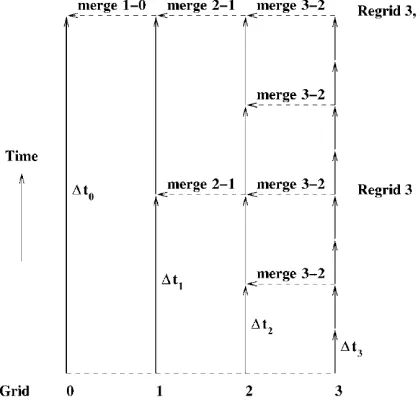
Integrate(0) then integrates all grids through one G0 grid timestep, t. This process is shown

schematically in Figure 2 for four grid levels. From the figure it can be seen that a coarse grid solution at the advanced time is available whenever a fine grid is integrated. This coarse grid solution provides a space-time interpolant that is used to impose the boundary conditions on the fine grid at a coarse-fine grid boundary.

The projection of the fine grid solution onto the coarse grid (the merge operation) simply involves replacing the coarse grid solution in a cell by the average of the solutions in the fine grid cells that it contains i.e.

Here(Pi n+1

)coarse is the coarse cell solution of the PDF in coarse celli at timetn and(Pk n+1

)fineis the fine cell solution in fine cellk at the same time.

Figure 1. Grid refinement at a region requiring high resolution (represented by thick black curve).

Figure 2. Integration of a four level grid.

2.4. Simple model for molecular mixing

Equation (2) only contains reaction terms, which has the advantage that it is easy to solve analytically. However, it lacks a crucial physical effect: molecular mixing as described in [2, 14]. There are a number of models for this, which we will explore further in Section 6. For the moment we replace (2) by

The third term of this equation is the linear mean square estimation closure (LMSE), which assumes that the turbulence is isotropic, homogeneous with constant density and that the initial PDF is normal. Here CD, and k are the ratio of the scalar to mechanical turbulent time scales,

the viscous dissipation rate of turbulence kinetic energy and the turbulence kinetic energy per unit mass (see [14] for details). Here we setCD/2k= 0.5 for two species and 0.35 for three species.

The LMSE term also describes advection, so it can be implemented by simply modifying the advection speed appropriately. For this we need , which involves calculating the ensemble

3. Monte Carlo Method

3.1. Simple reactive modeling

In order to compare AMR with Monte Carlo, we use a method of the same type as that described in [14, 20]. This is by no means the only choice, but it is typical of methods in widespread use. The PDF is now represented by an ensemble of stochastic particles and the value of the PDF at any point is obtained from the number of particles in a sample cell at that point, i.e.

where NP is the total number of particles,nP is the number of particles in a sample cell centred at

(1, … N)andis the volume of the sample cell. The motion of these particles is determined by

the reaction equations (1). This is equivalent to an Eulerian Monte Carlo scheme, as described in Möbuset al.[20].

Such a method is, of course, easier to implement than that described in Section 2 and it does not suffer from numerical diffusion. However, the accuracy depends both upon the number of particles and the size of the sample cell: for a given number of particles, the sample cell cannot be made so small that it only contains a few particles because this leads to unacceptable noise in the solution. As Sabel’nikov and Soulard [5] point out, this means that if one needs np particles per cell for a

good solution, then in N dimensions the total number of particles must be NP = (NC) N

np if the

number of cells in each direction isNC. This means that the computational cost of the Monte Carlo

method also increases exponentially with increasing number of speciesN.

It is evident that the choice of particle number and sample cell size is crucial for the performance of Monte Carlo methods. In order to show the method in its best light, we performed a number of experiments to determine the sample cell size that gave the best agreement with our initial PDF. Figures 3-6 show the results for the two species case discussed in Section 5.1.

3.2. Molecular mixing

In the Monte Carlo method, the LMSE model is equivalent to moving the particles towards the mean in composition space at a speed proportional to their distance from the mean. In this case the mean concentrationfor specieis given by

Figure 3. Monte Carlo with 2 species:Pversusaatb= 0.1 for time = 0.0 with 2002sample cells

(— = theory, = 3.2× 106particles, • =3 19,080 particles, = 31,343 particles).

Figure 4. Monte Carlo with 2 species:Pversusbata= 0.9 for time = 0.0 with 2002sample cells

(— = theory, = 3.2 × 106particles, • = 319,080 particles, = 31,343 particles).

Figure 5. Monte Carlo with 2 species:Pversusaatb= 0.1 for time = 0.0 with 4002particle sample

cells ( — = theory, = 1.2 × 107particles, • = 1.2 × 106particles, = 123,240 particles).

Figure 6. Monte Carlo with 2 species:Pversusbata= 0.9 for time = 0.0 with 4002particle sample cells

4. Test Cases

We start by considering two simple test cases for which it is possible to obtain an analytic solution to Equation (2).

4.1. Two species test case

This involves two chemical species that are represented by1=aand2=b, where the reaction isa

b. For the reaction rates we choose a simple isothermal autocatalytic form so that Equations (1) become

These imply that

Equation (2) then becomes

This can readily be solved by the method of characteristics, giving

along the characteristics given by

Equation (16) can be integrated to give

where (a0, b0)is the point on the characteristic at t= 0 which goes to (a, b) at timet. For a given

(a, b), (a0, b0) can be found in terms of(a, b) by integrating the characteristic equations (17) using

Equation (14). The result is

Equations (18) and (19) determine P at timet from the initial data. The initial data was a Gaussian centred ata=0.9,b=0.1 with a standard derivation of 0.025.

4.2. Three species test case

We now consider three chemical species represented by 1 = a, 2 = b and 3 = c, where the two

reactions area banda c. The reaction equations (1) are now

Equation (20 becomes

As in the previous case, this equation can readily be solved by the method of characteristics, giving

along the characteristics given by

Again, we can integrate (23) to get

where (a0, b0, c0) is the point on the characteristic at t=0 that goes to (a, b, c) at t. (a0,

b0, c0) can be found in terms of (a, b, c) by integrating the characteristic Equations (24) using

(21) to get

5. Results and Discussion

5.1. Monte Carlo method

As we have already pointed out in Section 3.1, it was necessary to perform some tests in order to ascertain how many particles were needed for an accurate representation of the initial Gaussian. This is, of course, not a problem for AMR.

Figures 3-6 show some results for the initial Gaussian for two species for different numbers of particles with 200 × 200 and 400 × 400 particle sample cells. It is clear that the Monte Carlo method can produce an accurate representation of the initial Gaussian, given a sufficient number of particles.

When molecular mixing is included, the end point of the evolution in both cases is a delta- function at the equilibrium state (a= 0, b= 1 for two species anda= 0, b=c = 0.5 for three species). Both the methods approximate this rather well and the AMR in particular becomes very fast as the region in which P differs significantly from zero shrinks. There is therefore little point in making comparisons at late times, instead we consider an intermediate time at which the solution is neither a Gaussian nor close to a delta-function. This is, of course, exactly the stage where one needs to model the PDF accurately.

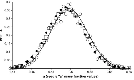
Figure 7 shows the results of a two species test att= 2.2 in a plane atb= 0.5. The equivalent result for three species is given in Figure 8 in a plane at b = c = 0.34. It can be seen that for the two species case, roughly 1.2 × 107 particles with 400 × 400 sample cells are required to obtain good agreement with the analytical theory. For three species, even with 5.0 × 108particles and 400 × 400 × 400 sample cells, the agreement is not so good: there is a distinct displacement from the theoretical curve. This is not surprising since the number of particles per sample cell is significantly smaller than for two species.

5.2. AMR method

The same initial conditions were used for the AMR test and the effect of varying the resolution by changing the number of grid levels was explored. From Figure 9, we can see that, for the two species case, a good solution can be obtained with six levels and a reasonable one with five levels, but that there is significant numerical diffusion with four levels. For the three species, Figure 10 shows similar results except that the agreement is not so good. The solution for six levels is of about the same quality as the Monte Carlo with 5 × 108particles. Note that, as for the Monte Carlo, the error at high resolution is a displacement from the theoretical curve, not simple diffusion as one would expect for uniform advection. This is because the non-linearity of the reactions distorts the original Gaussian.

5.3. Molecular mixing tests with Monte Carlo and AMR methods

Unfortunately, there is no simple analytic solution once we include the LMSE model for molecular mixing discussed in Section 2.4. The only way to assess the two methods is therefore to examine the rate of convergence. We can see from Figures 11 and 12 that, for two species, the Monte Carlo with 1.2 × 107particles and 400 × 400 sample cells gave a converged result with AMR with six levels of refinement. For three species, shown in Figures 13 and 14, 5.0 × 108particles and 400 × 400 × 400 sample cells for Monte Carlo give a similar result to that of AMR with six levels of refinement.

The molecular mixing effect for the two and three species cases required different values of the constant,CD/2k. This was necessary to achieve the same level of mixing for the two cases.

5.4. Run times and memory requirements

with molecular mixing and 1.1 without.

The advantages of AMR over a uniform grid can be seen by comparing the run times for two species with different numbers of grid levels. For a uniform grid this should increase by a factor of 8 when the grid is refined by a factor of 2, but for the two species AMR calculation it increases by a factor of about 2. The same is true of the memory requirements: for a uniform grid this should increase by a factor of 4 when the grid is refined by a factor of 2, but it only increases by about 1.3. The gains for the three species case are similar. However, AMR is not without costs: the number of cell updates per CPU second decreases as the number of levels is increased, but it never becomes smaller than that on a uniform grid by more than a factor of 2.

Monte Carlo is evidently not competitive with AMR for two species, although it does better with three. However, for three species the memory requirements for Monte Carlo are beginning to become prohibitive. In fact it is evident that this makes it difficult to obtain accurate results with Monte Carlo for more than a few species, whereas AMR does not suffer nearly so seriously from this limitation.

Figure 7. Monte Carlo with 2 species:Pversusaatb= 0.5 for time = 2.2 (— =theory, =1.2 × 107particles with

4002particle sample cells, • = 3.2 × 106particles with 2002particle sample cells, = 123,240 particles with 4002

particle sample cells).

Figure 8. Monte Carlo with 3 species:Pversus aatb=c= 0.34 for time = 2.2 ( — =theory,

= 5.0 × 108particles with 4003particle sample cells, • = 1.2 × 107particles with 4003particle sample

Figure 9. AMR with 2 species:Pversusaatb= 0.5 for time = 2.2 (—=theory,

= 6 levels, • = 5 levels, = 4 levels).

Figure 10. AMR with 3 species:Pversusaatb=c= 0.34 for time=2.2 ( — =theory,

= 6 levels, • = 5 levels, = 4 levels).

Figure 11. Monte Carlo and AMR with two species and molecular mixing:Pversusaatb= 0.5 for

time = 2.2 (— = AMR with six levels, = 1.2 × 107particles with 4002particle sample cells, • = 3.2 × 106

Figure 12. AMR and Monte Carlo with two species and molecular mixing:Pversusaatb= 0.5 for

time = 2.2 (— = Monte Carlo with 1.2 × 107particles with 4002particle sample cells, = AMR with 6

levels, • = AMR with 5 levels, = AMR with 4 levels).

Figure 13. Monte Carlo and AMR with three species and molecular mixing:Pversusaatb=c= 0.34 for

time = 2.2 (— =AMR with six levels, = 5.0 × 108particles with 4003particle sample cells, • = 3.2 × 107

particles with 2003particle sample cells, = 1.2 × 107particles with 4003particle sample cells).

Figure 14. AMR and Monte Carlo with three species and molecular mixing:Pversusaatb=c= 0.34

for time = 2.2 (— = Monte Carlo with 5.0 × 108particles with 4003particle sample cells, = AMR with

Table I. Run times for two species performed on a 3.06 GHz dual intel xenon processor workstation

(Timesteps: AMR=0.032, Monte Carlo(2002)=0.004, Monte Carlo(4002)=0.002).

Type of scheme Field resolution CPU (s) Memory (GB)

AMR (6 levels + molecular mixing) 252coarse cells 40 0.042

AMR (6 levels) 252coarse cells 28 0.042

AMR (5 levels + molecular mixing) 252coarse cells 20.5 0.03

AMR( 5 levels) 252coarse cells 18 0.03

AMR (4 levels + molecular mixing) 252coarse cells 10 0.027

AMR (4 levels) 252coarse cells 7 0.027

Monte Carlo + molecular mixing 4002samples

1.2 × 107particles 1660 0.78

Monte Carlo 4002samples

1.2 × 107particles 1335 0.78

Monte Carlo + molecular mixing 2002samples

3.2 × 106particles 211 0.21

Monte Carlo 2002samples

3.2 × 106particles 170 0.21

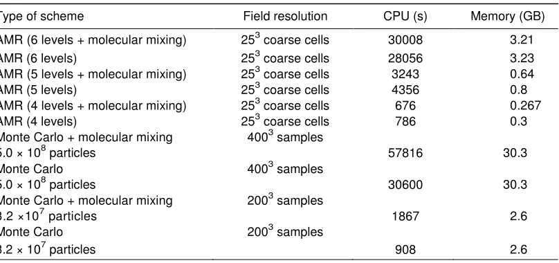
Table II. Run times for three species performed on an AMD cluster opteron 848 at 2 GHz

(Timesteps: AMR = 0.032, Monte Carlo(2003)=0.004, Monte Carlo(4003)=0.002).

Type of scheme Field resolution CPU (s) Memory (GB)

AMR (6 levels + molecular mixing) 253coarse cells 30008 3.21

AMR (6 levels) 253coarse cells 28056 3.23

AMR (5 levels + molecular mixing) 253coarse cells 3243 0.64

AMR (5 levels) 253coarse cells 4356 0.8

AMR (4 levels + molecular mixing) 253coarse cells 676 0.267

AMR (4 levels) 253coarse cells 786 0.3

Monte Carlo + molecular mixing 4003samples

5.0 × 108particles 57816 30.3

Monte Carlo 4003samples

5.0 × 108particles 30600 30.3

Monte Carlo + molecular mixing 2003samples

3.2 ×107particles 1867 2.6

Monte Carlo 2003samples

3.2 × 107particles 908 2.6

6. Tests with Different Molecular Mixing Models

So far we have only considered the LMSE model for molecular mixing, but as we have already pointed out in Section 2.4, there are other possibilities: the coalescent/dispersal model or Curl model [21]; the Langevin model or Fokker-Planck equation [2]. In order to keep things simple, we consider the evolution of two delta-functions, approximated by narrow Gaussians, in one dimension with no reactions. The initial conditions are

where1= 0.1,2= 0.9,= 0.008.

6.1. LMSE model

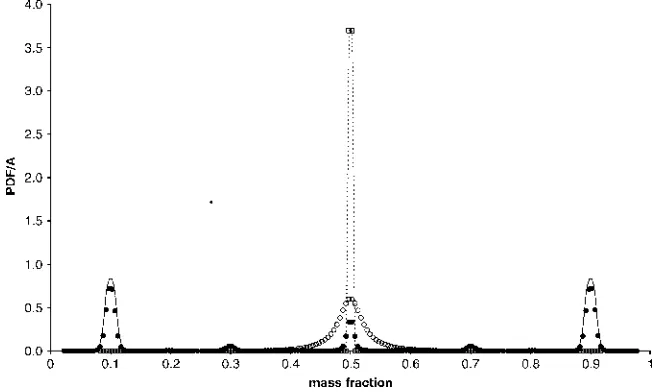
The time evolution in this case is very simple: each Gaussian moves towards the mean  = 0.5 with a speed proportional to its distance from the mean. Figure 15 shows that this is exactly what happens. The narrow Gaussians spread out somewhat due to numerical diffusion while they are moving, but the end result is a very good approximation to a delta-function at  = 0.5. This is in stark contrast to the results obtained by Kosaly [22] for this problem with Monte Carlo using 2  104 particles. Kosaly’s results are rather surprising since it ought to be possible to do this particular case almost exactly with Monte Carlo by simply placing a particle at the initial positions of the delta-functions.

Figure 15. Probability density functions versus concentration at different time evolution stages for linear mean square estimation closure model (— = Initial PDF distribution,

• = stage 1, = stage 2, - - - =stage 3).

6.2. Curl model

In a simple version of the Curl or coalescence/dispersal model, the equation forPbecomes

whereCQ is the ratio of the decay time scale of velocity fluctuations to the decay time scale of scalar

fluctuations. From Pope [2]CQis usually 2.0. One has to be slightly careful of how one approximates

(29):Pis not conserved if the two terms on the RHS are treated separately. However, conservation is guaranteed if one approximates the integrals in the equivalent equation

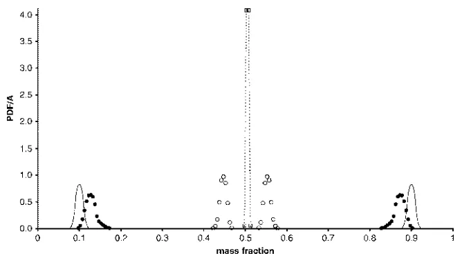
Figure 16 shows the evolution for this case, which clearly indicates the unphysical nature of this model: it recursively produces a series of Gaussians at the mid-points between the existing delta-functions. The solution does eventually evolve into a delta-function at the mean value, but as Kosaly points out [22], it would never be formally smooth if the initial condition contains delta-functions. Although it is possible to add a kernel to the integrals that removes this problem [3, 23], this model has no obvious advantages. It is also very expensive for both AMR and Monte Carlo since it involves an integro-differential equation.

large number of particles would be needed to get a good approximation to the heights of the delta-functions. Despite this, Kosaly’s results for this problem are rather poor.

Figure 16. Probability density functions versus concentration at different times for the Curl molecular

mixing model (— = Initial PDF distribution, • = first stage, = second stage 2, - - - = final stage).

6.3. Langevin model

The most natural model for molecular mixing is the Langevin model, which adds diffusion to the LMSE model to produce a Fokker-Planck equation. The equation forPis then

where 2 is the variance at time t. In order to ensure that the variance decays in the correct manner, we must have [2]

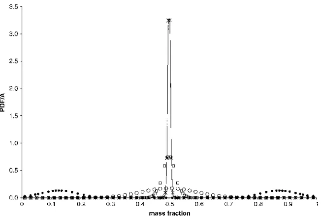
Figure 17 shows that the initial Gaussians are immediately spread by the diffusion, but the decay in the variance eventually ensures that P evolves to a delta-function at the mean value of . In contrast to the other models, P is smooth during most of the evolution, but AMR can still give significant gains because it is still only significant in a small part of the domain. Note that although Pope regards this model as satisfactory in all respects, he claims that it is unsuitable for compositions since the implementation of diffusion in Monte Carlo can lead toPbeing non-zero for unphysical compositions. This is not a problem for finite-volume since the boundary conditions ensure that there is no flux ofPoutside the range of physically realisable compositions.

Figure 17. Probability density functions versus concentration for the Langevin molecular mixing with

different stages of diffusion (• = stage 1, = stage 2, = stage 3, × — = stage 4).

7. Conclusions

The purpose of this paper was to show that finite-volume methods combined with AMR provide an attractive alternative to Monte Carlo for solving the transported PDF equation. We have deliberately considered rather simple cases in order to compare our numerical solutions either with analytic ones or with fully converged numerical solutions. Despite the simplicity of these problems, they include generic features that are relevant to real applications: non-linear reactions; molecular mixing. We have not considered cases with space dependence, although not only is our AMR code capable of this, but the refinement in space would give it a further advantage over Monte Carlo. This is because we simply could not carry out Monte Carlo calculations with space dependence that gave a reasonable level of accuracy. In fact our results show that the memory requirements for the type of Monte Carlo method used are such that it is incapable of producing accurate solutions for the PDF in all but the simplest of situations. This conclusion is borne out by the very few tests of Monte Carlo against known solutions that have appeared in the literature (e.g. [22]).

It would seem that our results lead to a rather grim conclusion: both AMR and Monte Carlo need far higher resolution to produce accurate solutions to the PDF equation than one could possibly achieve in any realistic case. AMR can do much better than Monte Carlo in a calculation that includes the flow field, even though it could not possibly cope with more than a few active species. The only hope is that a few species is sufficient or that good results can be obtained even with a poor solution to the PDF equation.

Acknowledgements

References

1. Schildmacher KU, Hoffmann A, Selle L, Koch R, Schulz C, Bauer HJ, Poinsot T, Krebs W, Prade B. Unsteady flame and flow field interaction of a premixed model gas turbine burner.

Proceedings of the Combustion Institute2007;31(2): 3197-3205.

2. Pope SB. PDF methods for turbulent reactive flows. Progress in Energy and Combustion Science1985;11: 119-192.

3. Janicka J, Kolbe W, Kollmann W. Closure of transport equation for the probability density function of turbulent scalar fields. Journal of Non-Equilibrium Thermodynamics1979; 4: 47-66.

4. Janicka J, Kolbe W, Kollmann W. The solution of a PDF-transport equation for turbulent diffusion. In Proceedings of the Heat Transfer and Fluid Mechanics Institute, Crowe CT, Grosshandler WL (eds). 1978; 297-312.

5. Sabel’nikov V, Soulard O. Rapidly decorrelating velocity-field model as a tool for solving one-point Fokker-Planck equations for probability density functions of turbulent reactive scalars.

Physical Review E2005;72: 16301-163022.

6. Berger MJ, Oliger J. Adaptive mesh refinement for hyperbolic partial differential equations.

Journal of Computational Physics1984;53: 484-512.

7. Berger MJ, Colella P. Local adaptive mesh refinement for shock hydrodynamics. Journal of Computational Physics1989;82: 64-84.

8. Bell J, Berger M, Saltzmann J, Welcome M. Three dimensional adaptive mesh refinement for hyperbolic conservation laws. Society for Industrial and Applied Mathematics Journal on Scientific Computing1994; 15: 127-138.

9. Quirk JJ. A parallel adaptive grid algorithm for computational shock hydrodynamics. Applied Numerical Mathematics1996;20: 427-453.

10. Online details of CHOMBO code: http://seesar.lbl.gov/ANAG/chombo/. 11. Online details of FLASH code: http://flash.uchicago.edu/website/home/. 12. Online details of SAMRAI code: http://www.llnl.gov/CASC/SAMRAI/.

13. Fromang S, Hennebelle P, Teyssier R. A high order Godunov scheme with constrained transport and adaptive mesh refinement for astrophysical magnetohydrodynamics.

Astronomy and Astrophysics2006;457: 371-384.

14. Jones WP, Kakhi M. Pdf modelling of finite-rate chemistry effects in turbulent nonpremixed jet flames.Combustion and Flame1998;115: 210-229.

15. Godunov SK. Finite difference methods for numerical computations of discontinuous solutions of the equations of fluid dynamics. Matematicheski Sbornik 1959; 47(89): 271-306.

16. Falle SAEG. Self-similar jets. Monthly Notices of the Royal Astronomical Society 1991; 250: 581-596.

17. Online details of AMROC code: http://amroc.sourceforge.net/.

18. Baum JD, Löhner R. Numerical simulation of shock-elevated box interaction using an adaptive finite shock capturing scheme.American Institute of Aeronautics and Astronautics,

AIAA-1989-653, 1989.

19. Khkhlov AM. Fully threaded tree algorithm for adaptive refinement fluid dynamics simulations.Journal of Computational Physics1998;143: 519-543.

20. Möbus H, Gerlinger P, Brüggemann D. Comparison of Eulerian and Lagrangian Monte Carlo

PDFmethods for turbulent diffusion flames.Combustion and Flame 2001;124:(3): 519-534. 21. Curl RL. Dispersed phase mixing: 1 theory and effects in simple reactors.AIChE Journal 1963;

9(2): 175-181.

22. Kosaly G. Modelling of turbulent molecular mixing.Combustion and Flame1987;70: 101-118. 23. Dopazo C. Relaxation of initial probability density functions in turbulent convection of scalar