Evidence-based robust optimisation of space systems with evidence network models

Evidence-Based Robust Optimisation of Space

Systems with Evidence Network Models

Gianluca Filippi

Department of Mechanical & Aerospace Engineering University of Strathclyde, Glasgow, UK

Email: [email protected]

Mariapia Marchi

ESTECO SpA, Trieste, IT Email: [email protected]

Massimiliano Vasile

Department of Mechanical & Aerospace Engineering University of Strathclyde, Glasgow, UK Email: [email protected]

Paolo Vercesi

ESTECO SpA, Trieste, IT Email: [email protected]

Abstract—The paper presents an approach to optimise complex systems in space systems engineering, accounting for epistemic uncertainty. Uncertainty is modelled with Dempster-Shafer the-ory of Evidence and the space system as a network of connected components. A constrained min-max problem is then solved, with a memetic algorithm, to deliver a robust design point. Starting from this robust design point a sequence of evolutionary optimisation steps are used to reconstruct an approximation of the Belief and Plausibility curves associated to a particular design solution. The constrained min-max approach and the evolutionary reconstruction of the Belief and Plausibility curves are tested on a realistic case study of space systems engineering.

I. INTRODUCTION

Space systems engineering aims at designing, developing and verifying a system that can operate in space. This system is made of a number of interconnected components or subsys-tems, each of which performs a number of tasks, has inputs and outputs shared with other components and is qualified by a number of attributes. The failure or under-performance of one or more components affects the whole system and can lead to a system failure.

In the early design phase, one main point of concern is to evaluate the overall performance or attribute of the whole system. Typically a performance metric is the overall mass of the system but other attributes can become key performance indicators, like the data volume or the power output.

One critical aspect in the evaluation of particular systems engineering solution is the reliability of the value associated to a given performance metric. In fact, due to the uncertainty in the requirements, operational conditions, model parameters, component characteristics, etc. a deterministic design solution might not provide a reliable result.

The uncertainty introduced at an early design stage is mainly epistemic and require an appropriate treatment [1][2]. This paper starts from the concept of Evidence Network Models, recently introduced in [3], and extends previous work to in-troduce constraints in the system definition and operations. In Evidence Network Models, epistemic uncertainty are modelled

as Belief functions and two values (Belief and Plausibility) are associated to the value of the system performance [4].

The resulting system optimisation under uncertainty process is composed of the solution of a constrained bi-level min-max optimisation problem followed by the reconstruction of the Belief and Plausibility on the value of the performance metric. The constrained min-max problem is a variation of the unconstrained approach presented in [5] and its solution is here addressed with a modification of Inflationary Differential Evolution [6] implemented in the software code MPAIDEA [7]. MPAIDEA is then used to provide an approximation to the Belief curves following the h-decomposition process proposed in [8]. The paper is structured as follows. After introducing some fundamentals on Evidence Network Models, the paper presents the strategy to solve the constrained min-max problem and the h-decomposition approach. Results on a real-world test case will then follow.

II. EVIDENCENETWORKMODELS

A generic complex system can be represented as a network, where each node is a subsystem and information is shared through links between subsystems. We can then define a functionF as

F(d,u) =

N

X

i=1

gi(d,ui,hi(d,ui,uij)) (1)

whereNis the number of subsystems involved,hi(d,ui,uij)

is the vector of scalar functions hij(d,ui,uij) where j ∈ Ji and Ji is the set of indexes of nodes connected to the i-th node; ui are the uncertain variables of subsystem i not

shared with any other subsystem and uij are the uncertain

variables shared among subsystems i andj. Please note that according to our notationuij =ujiand the functionsgi(·,·,·)

g1(d,u1,u12,u13)

g2(d,u2,u12,u23) g3(d,u3,u13,u23)

u12 u13

u23

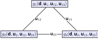
Fig. 1. Evidence Network Model of a generic systemF composed of three sub-systems with coupled variablesu12,u13andu23.

the different subsystems. In a fully connected network as in Figure 1 the function F is:

F(d,u) = g1(d,u1, h12(d,u1,u12), h13(d,u1,u13))+ g2(d,u2, h21(d,u2,u12), h23(d,u2,u23))+ g3(d,u3, h31(d,u3,u13), h32(d,u3,u23)).

(2) We then callui,uncoupledvariables because they influence

only one subsystem and uij coupled variables because they

influence two subsystems. Hence, for the example in Figure 1, the uncertain vector can be ordered as

u= [u1,u2,u3,u12,u13,u23]T.

In the following we will study only the case of functions

gi(·,·,·)that are always positive semi-definite and monotonic

with respect to each functionhik.

Given a design, or decision, value˜d∈D we will callworst

case scenario the vectoruthat corresponds to the maximum

of F over the spaceU:

u= argmax

u∈U

F(ed,u). (3)

Likewise we can callbest case scenariothe quantity:

¯

u= argmin

u∈U

F(ed,u). (4)

We can now define an event in the spaceU, or a proposition on the value of F, as the setAsuch that:

A={u∈U|F(d,u)≤ν}. (5)

From this definition it is clear that for every design d∈ D

the worst case scenario corresponds to A=U, becauseν = maxu∈UF(d,u), and analogously the best case scenario has

zero measure. Each uncoupled uncertain vector ui is defined

over a set of boxes named Θi = ∪kθk,i and each coupled

uncertain vector uij is defined over the set of boxes Θij =

∪kθk,ij. We define the set

Θ =[

i

θi= (×mi=1uΘi)×(×mi,jc=1Θij)

wheremuis the number of uncoupled uncertain vectors (equal

to the number of subsystems) andmcis the number of coupled

uncertain vectors. In this context, the hyperpower set

DΘ= (Θ,∪,∩) (6)

is the set composed of the elements of Θ, their union and intersection. In the following the spaceU :=DΘ_{. We can then}

define two quantities associated to the belief in the occurrence of the eventA:

Bel(A) = X

θ⊂A,θ∈U

bpa(θ) (7)

P l(A) = X

θ∩A6=0,θ∈U

bpa(θ) (8)

where bpa(θ) is the basic probability assignment associated toθ, an element of the power set [4]. It is important to note that if thehij functions were known with certainty the nodes

composing the network would be decoupled and statistically independent. We also note that in order to identify if a θ is fully included inA we need to find the maximum ofF with respect to u ∈ θ. Likewise an intersection with A requires computing the minimum of F with respect to u∈θ. Given that the subsets θ, their unions and intersections come from a cross product, it is clear that the number of maximisation and minimisation increases exponentially with the number of dimensions. The computation of the Belief Bel (Plausibility

P l respectively) in the occurrence of A is, therefore, an exponentially complex operation. In the following section a technique is proposed to compute an approximation to (7) by exploiting some of the properties of the ENM listed above. In particular we will exploit the following three properties:

1) The contribution of the coupled variableuij to the value F manifests through the scalar functions hij andhji.

2) Allgi functions are positive semi-definite.

3) All gi functions are monotonically increasing with

re-spect tohij for every j.

III. CONSTRAINEDMINMAX

The approach to the design of complex systems under uncertainty proposed in this paper, requires the solution of one or more constrained min-max optimisation problems. The solution to this class of problem is here approached with a constrained variant of MPAIDEA, an adaptive version of Inflationary Differential Evolution [7]. This section describes only the strategy to handle constraints in the min-max version of MPAIDEA. More details on the approach to the solution of unconstrained min-max problems with Inflationary Differential Evolution can be found in [9].

A. Memetic Approach

The min-max algorithm proposed in this paper iteratively solves a bi-level optimisation, first minimising over the design vectord(outer loop) and then maximising over the uncertainty vector u(inner loop). The inner loop provides solutions that satisfy the constraint, while the outer loop maintains the constraint satisfaction while minimising the cost function F. The constraint handling procedure, summarised in Algorithm 1, implements the following steps:

• While the number function evaluations is lower than

Nmax

f eval function evaluations, do the following

– [Outer Loop] Constrained minimisation of the ob-jective function over the design space, evaluating the cost functionF over all the uncertainty vectors stored in an archive A=Au∪Ac:

mind∈D∧u∈AF(d,u) s.t.

maxu∈AC(d,u)≤0

(9)

– [Inner Loop] Constrained maximisation of the cost function F over the uncertain parameters u and parallel maximisation of the constraint violation over the uncertainty space:

maxu∈UF(dmin,u) s.t.

C(d,u)≤0

(10)

max

u∈U C(dmin,u) (11)

ua,F = argmaxu∈UF(dmin,u) is added to the

archive Au and ua,C = argmaxu∈UC(dmin,u) is

added toAc ifmaxu∈UC(d,u)>0. This approach

pushes the optimiser to find design configurations that are feasible for all values of the uncertain variables. If a feasible solution cannot be found, the constraints are relaxed (line 15), in the Inner Loop, by computing the new constraintC∗ =C+with

the minimum constraint violation overU.

In the multi-objective optimisation:

• Cross-check of the final solutions and choice of the best design;

• Final maximisation over U.

IV. DECOMPOSITIONALGORITHM

In order to reduce the computational complexity of the calculation ofBel(A)we propose a decomposition technique that exploits the three properties defined in the previous sec-tion. The decomposition algorithm aims at decoupling the sub-systems over the uncertain variables in order to optimise only over a small sub-set of the Focal Elements (FEs) (Algorithm 2); this procedure requires the following steps:

1) Solution of the optimal worst case scenario problems (9),(10) and (11).

2) Maximisation over the coupled variables and computa-tion ofmc partial Belc(A)curves.

3) Maximisation over the uncoupled variables. 4) Reconstruction of the approximation Belg(A).

The result of the solution of problems (9),(10) and (11), as presented in section III, are the values d˜ and u, thus, in the following, the decomposition starts once d˜ andu are available. However, it has to be noted that a Belief curve can be computed for any arbitrary d.

Algorithm 1 Constrained minmax

1: Initialise d¯ at random and run ua = argmaxF(¯d,u)s.t. C(dmin,u)≤0

2: Au=Au∪ {ua}; Ac=∅;Ad=∅

3: while Nf val< Nf valmaxdo

4: Outer loop:

5: dmin= argmind∈D{maxu∈Au∪AcF(d,u)} s.t.

maxu∈Au∪AcC(d,u)≤0

6: Ad=Ad∪ {dmin}

7: Inner loop:

8: ua,F = argmaxu∈UF(dmin,u)s.t.C(dmin,u)≤0

9: ua,C= argmaxu∈UC(dmin,u)

10: Au=Au∪ {ua,F}

11: if Nf val< Nf valrelaxation∨

∃d∈Ad t.c.maxu∈UC(d,u)≤0 then

12: if maxu∈UC(dmin,u)>0then

13: Ac =Ac∪ {ua,C}

14: end if

15: else

16: update

17: Ac ={Ac\ua,C|C(dmin,u)≤}

18: if maxu∈UC(dmin,u)> then

19: Ac =Ac∪ {ua,C}

20: end if

21: end if

22: end while

A. Maximisation over the coupled variables and evaluation of the partial Belief curves

For each coupled vectoruij a maximisation is run over each

FE θk,ij ⊆Θij ⊆U, givened and keeping fixed all the other components of u. Taking again the example in Figure 1 we have:

ˆ

uk,12= argmax u12∈θk,12

F(ed,u₁,u₂,u₃,u12,u13,u23),∀θk,12⊂Θ12

ˆ

uk,13= argmax u13∈θk,13

F(ed,u1,u2,u3,u12,u13,u23),∀θk,13⊂Θ13

ˆ

uk,23= argmax u23∈θk,23

F(ed,u₁,u₂,u₃,u₁₂,u₁₃,u23),∀θk,23⊂Θ23

(12)

For the sake of simplicity we will indicate with

F(uij) :=F(˜d,u1, ...,uij, ...,ui+1j, ...).

We can then compute the partial belief associated only to the coupled variables with indexij:

Bel(F(uij)< ν) =

X

θk,ij|maxuij∈θk,ijF(uij)≤ν

bpa(θk,ij).

the corresponding values of the coupled vectors _buq_k,ij. These values will be used in the next step to decouple the functions

gi and compute the maxima of each gi with respect to the

uncoupled variables ui.

B. Optimisation over the uncoupled vectors

For each νq, given a fixed value of the coupling functions,

one can study each gi independently of the others. The idea

is to run an optimisation for each function gi over only the

uncoupled vector ui. With the example in Figure 1 in mind,

having

ˆ

hq_ij(ui) :=hij(˜d,ui,uˆ q ij)

where uˆq_ij := ˆuq_k∗_,ij :k∗ = argmaxkF(ˆu q

k,ij), is one of the

maxima of the maxima attained by the coupled variable uij.

For every FE θk,i∈Θi we have:

ˆ

uq_k,1= argmax

u1∈θk,1

g1(ed,u1,bh

q

12(u1),bh

q

13(u1)),∀θk,1⊂Θ1

ˆ

uq_k,2= argmax

u2∈θk,2

g2(ed,u2,bh

q

21(u2),bh

q

23(u2)),∀θk,2⊂Θ2

ˆ

uq_k,3= argmax

u3∈θk,3

g3(ed,u3,bh

q

31(u3),bh

q

32(u3)),∀θk,3⊂Θ3

(14)

with the corresponding values ˆgq_k,1,gˆq_k,2 andgˆq_k,3.

C. Complexity Analysis

From the definition of the hyperpower set in (6) it is clear that the number of focal elements increases exponentially with the number of dimensions. Even if one limits the U space to the sole Θ the total number of FEs for a problem with m

uncertain variables, each defined over Nk intervals, is:

NF E = m

Y

k=1

Nk. (15)

In terms of coupled and uncoupled uncertain vectors we can write:

NF E=





mu

Y

i=1 pu_i

Y

k=1 N_i,ku

    mc Y i=1 pc_i

Y

k=1 N_i,kc



 (16)

wherepu_i andpc_i are the number of components of thei−th

uncoupled and coupled vector, respectively, andN_i,ku andN_i,kc

are the numbers of intervals of the k−thcomponents of the

i−th uncoupled and coupled vector respectively. The total number of focal elements that needs to be explored in the decomposition is instead:

NF EDec=Ns mu

X

i=1

NF E,iu + mc

X

i=1

NF E,ic (17)

considering the vector of uncertainties ordered as

u= [u1, ...,umu

| {z }

uncoupled

,u1, ...,umc

| {z }

coupled

]

where and Ns is the number of samples in the partial belief

curves, Nc F E,i =

Qpci

k=1N c

i,k and NF E,iu =

Qpui

k=1N u i,k.

This means that the computational complexity to calculate the maxima of the function F within the focal elements is polynomial with the number of subsystems and remains exponential for each individual uncoupled or coupled vector.

D. Reconstruction

Once all the maxima over the focal elements of the uncoupled variables are available for each sample q one can calculate an approximation of Bel(F(d,u) < ν) as follows. From Eq. (14), for each sample q the maximum associated to focal element θk = θk1,1 ×θk2,2×θk3,3, for k= 1, ...NF E,1·NF E,2·NF E,3, using a positive semi-definite gi, is:

max

(u1,u2,u3)∈θk

F(˜d,u1,u2,u3,uˆq12,uˆ q 13,uˆ

q 23) = ˆg

q k1,1+ ˆg

q k2,2+ ˆg

q k3,3

(18)

with associated basic probability assignment:

bpaq(θk) =bpa(θk1,1)bpa(θk2,2)bpa(θk3,3)∆Belq (19)

where ∆Belq = Q

ij∆Bel q

ij are the contributions of the

partial belief curves in (13). In other words, thebpaof eachθk

is the product of all the bpa’s of the FEs of each uncoupled variable scaled with the product of the belief values of the samples drawn from the partial belief curves (Line 18). The approximation of the belief is then computed as:

g

Bel(F(d,u)≤ν) =X

q

X

k

bpaq(θk). (20)

If the decomposition drastically reduces the number of maximisations, the reconstruction still requires an exponential number of multiplications of bpa’s. Thus, the computational cost of the reconstruction step would increase exponentially with the number of sub-systems if the full curve was required. In this case the number of times that (19) has to be evaluated is:

Nevals=Ns mu

Y

i=1

NF E,iu . (21)

If the decomposition is used to evaluateBel(F(d,u)< ν), for a given d and a single threshold ν, then a partial belief curve could be reconstructed only in a neighbourhood ofν at a reduced computational cost.

For a given sampleq, consider the vector

ˆ

gq_i = [ˆg_i,q₁, ...,gˆq_i,Nu F E,i]

T

of all the maxima of a functiongi over all the focal elements θk,i and the collection of vectors

Γ = [γqik] _{q = 1, ..., N} S i = 1, ..., mu k = 1, ..., Nu

F E,i

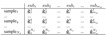
organised as in Table I. The approximated belief curve in Eq. (20) can be computed by taking the sum of the bpa’s for every row ofΓ and then adding up all the rows.

Now, given ν, one can filter out all the componentsgˆ_k,iq of each vectorgˆq_i that satisfies the relationship:

ˆ

g_k,iq +

NU

X

i=1

min

k ˆg q

i > ν. (22)

If condition (22) is applied to every vector in Γ we obtain a new collectionΓL. Symmetrically we can also construct the

collection ΓR by filtering the vectors inΓwith the following

condition:

ˆ

gq_k,i+

NU

X

i=1

max

k ˆg q

i < ν. (23)

The computation of Bel(F(d,u)≤ν)is realised by taking from each row of the two collections ΓL and ΓR the rows

with the least amount of focal elements, i.e. the ˆgq_i vectors with the lowest number of components, and form the new collection Γν. We can now calculate the approximated belief

as in Eq.(20) but using the rows and columns of matrix Γν.

TABLE I

INFORMATION USED IN THE RECONSTRUCTION STEP

sub1 sub2 ... subi ... submu

sample1 ˆg11 ˆg21 ... ˆg1i ... ˆg1mu

... ... ... ... ... ... ...

sampleq ˆgq1 ˆg q

2 ... ˆg

q

i ... ˆg q mu

... ... ... ... ... ... ...

sampleNs ˆg Ns

1 ˆg

Ns

2 ... ˆg

Ns

i ... ˆg Ns mu

The reconstruction computational cost after filtering is:

Nevals= Ns

X

q=1 mu

Y

i=1

dim(ˆg_iq), ˆgq_i ∈Γν. (24)

E. Simple example of the decomposition approach

Consider the equation F = g1+g2 where g1 = 10u21+

|u2|u25+ u4₆

100+d1|d2|andg2=|u3|+u 2 4

|u5| 10 +u

2

6+|d1|where

there are two uncoupled vectors (u1 = (u1, u2) and u2 =

(u3, u4)) and one coupled vector (u12= (u5, u6)). The

min-max solution ised= [−5,−5]∧u= [−5,−5,−5,−5,−5,−5] and the decomposition belief curves are presented in Fig. 2. Other simple test cases can be found in [3].

V. CASESTUDY

A. Optimal Battery Sizing

The minmax and h-decomposition approaches are here applied to the sizing of a battery on board a spacecraft during an orbital transfer from Geo Transfer Orbit to geostationary orbit (GEO)[11]. The goal is the constrained minimisation of the mass of the battery under epistemic uncertainty. The mass of the battery is dependent on the following design, uncertain and fixed parameters:

Algorithm 2 Decomposition

1: Initialise

2: Uncoupled vectorsuu= [u1,u2, ...,ui, ...,umu]

3: Coupled vectorsuc= [u12,u13, ...,uij, ...,umc]

4: fora given designde do

5: Compute (ed,u_u,u_c) =argmaxF(ed,u_u,uc)

6: foralluij ∈uc do

7: forall FEθk,ij ⊆Θij do

8: Fbk,ij = maxuij∈θk,ijF(ed,uu,uij)

9: u_bk,ij = argmaxuij∈θk,ijF

10: Evaluatebpa(θk,ij)

11: Evaluate partial Belief curve Bel(F(uij)≤ν)

12: end for

13: fornumber of samplesdo

14: Evaluate∆Belq_,

b

uk,ij andFbk,ij

15: end for

16: end for

17: forall the combinations of samples do

18: forallui∈uu do

19: forall FEθk,i⊆Θi do

20: Fmax,k,i= maxui∈θk,iF(ed,ubc,ui) 21: Evaluatebpa(θk,i)

22: end for

23: end for

24: forall the combinations of FE

θt∈Θ1×Θ2×...×Θmu do

25: EvaluateFmax,k≤ν

26: Evaluatebpak

27: end for

28: Evaluate the Belief for this sample by constructing collectionΓν

29: end for

30: Add up all belief values for all samples 31: end for

TABLE II

DESIGN PARAMETERS FOR BATTERY PROBLEM

variable symbol value insertion time t [6939.8 7304.8]

battery type γ [0, 1] Bus voltage ∆VBU S [0, 5]

• 3 design parameters. Time of orbit insertiont, type of battery γ and bus voltage∆Vbus:

d=t, γ,∆Vbus

T

.

Table II shows the design parameters with their associated range of variability: t is given in Modified Julian Date (MJD) - for more details see [11] - and can be any day of 2019 at 7 a.m.;γranges in four possible intervals - [0, 0.25) , [0.25, 0.5), [0.5 0.75) and [0.75, 1] - corresponding to 4 battery types (see Table III).

• 31 uncertain parameters. Orbital parameters of five orbitsα - semimajor axis,a, eccentricity,e, Inclination,

0 50 100 150 200 250 300 350 400 450 objective function

0 0.1 0.2 0.3 0.4 0.5 0.6 0.7 0.8 0.9 1

Belief

exact Belief 1 sample 2 samples 3 samples 4 samples 5 samples 6 samples

Fig. 2. Simple example of application of the decomposition approach

TABLE III

LOOKUP TABLE OF BATTERIES

BATTERY A B C D

Cell capacityCcell (Ah) 4.5 1.7 1.5 3.7

Cell voltage∆Vcell (V) 4.1 4.2 4.2 4.1

Cell Massm(γ)(kg) 0.63 0.2 0.21 0.23 Max DoDDoDmax(%) 80 75 75 75

of Perigee,ω and True Anomaly,θ(for more details see [11])- and efficiency of the battery η:

u=

α, η =

a,e,i,Ω,ω,θ, η]

with:

a = [a1, a2, a3, a4, a5]T,e = [e1, e2, e3, e4, e5]T,i =

[i1, i2, i3, i4, i5]T,Ω = [Ω1,Ω2,Ω3,Ω4,Ω5]T,ω =

[ω1, ω2, ω3, ω4, ω5]T,andθ= [θ1, θ2, θ3, θ4, θ5]T.

For each uncertain variable, two possible intervals are given, both with 50% of probability. They are symmet-rically arranged on either side of the nominal values in Table V; the interval dimensions are given by Table IV.

TABLE IV

UNCERTAIN INTERVALS

a (km) e (-) i (◦) Ω(◦) ω(◦) θ(◦) ∆u ±20 km ±0.0012 ±0.07◦ ±30◦ ±0.5◦ ±0.025◦

• 10 fixed parameters. Engine ignition time and Liquid

Apogee Engine (LAE) burn time per orbit (Table VI).

TABLE V

NOMINAL VALUE OF THE EPISTEMIC PARAMETERS FORSSTLPROBLEM

orbit a (km) e (-) i (◦) Ω(◦) ω(◦) θ(◦) 1 68500.3 0.90 22.81 86.63 180.10 0.00 2 73250.2 0.77 9.12 86.79 180.6 180.08 3 86065.5 0.51 1.09 85.96 180.81 180.84 4 49646.4 0.15 0.36 86.85 180.97 4.25 5 42049.0 0.001 0.05 270 0.00 359.95

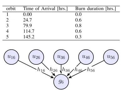
TABLE VI

FIXED PARAMETERS

orbit Time of Arrival [hrs.] Burn duration [hrs.]

1 0.00 0.0

2 24.7 0.6

3 79.9 0.8

4 114.7 0.6

5 145.2 0.3

u16 u26 u36 u46 u56

g6

h16 h26 h36 h46 h56

Fig. 3. Evidence Network Model of the optimal battery sizing problem.

The minmax problem is the constrained minimisation of the mass of the battery M under uncertainty:

min

d∈Dmaxu∈U M(d,u) s.t. C(d,u)<0. (25)

M depends on the mass of the cell (Table III) and on the total number of cells of the battery:

M =m(γ)Ntot (26)

and Ntot is the product of the number of cells in series Ns

and in parallel Np:

Ntot=NsNp=

∆VBU S

∆Vcell

E

DoDmax∆VBU SCcell

+ 1 (27)

whereE, the Energy requirement, depends on the length of the eclipse periods evaluated from the input data,∆VBU S is the

Bus voltage,∆Vcell the cell voltage,DoDmaxthe maximum

allowed Depth of Discharge, Ccell the Cell Capacity [10].

The constraint is given by the maximum allowed Depth of discharge for each type of battery (Table III):

C(d,u) (

>0 ifDoD(d,u)> DoDmax <0 ifDoD(d,u)< DoDmax

B. Evidence Network Model of the Battery Sizing Problem

The above-described battery sizing problem is modelled with an ENM assuming that each of the five orbits is a node of the network and all five nodes are connected to a6th_{node, the}

battery. The scheme of Fig. 3 illustrates this simple topology:

M(d,u) =

6

X

i=1

gi(d,ui,hi(d,ui,uij)) (28)

• 5 nodes evaluate the energy required by the spacecraft in the given orbits: Ei(d, ai, ei, ii,Ωi, ωi, θi) and have gi= 0 fori= 1,2, ...,5

• The 6th node sizes the mass of the battery:

The epistemic vector has been organised as:

u= [ u6

|{z}

uncoupled

,u16,u26,u36,u46,u56

| {z }

coupled

]

where: u6 = η and ui6 = [ai, ei, ii,Ωi, ωi, θi]T with i =

1,...,5.

Θ6=∪kθk,63u6 is the set of all the FE of the uncoupled

vector u6 andΘi6=∪kθk,i63ui6 is the set of all the FE of

the coupled vector ui6 for i=1, 2, ..., 5.

In the ENM model of this problem the five orbits indepen-dently contribute to the mass as the uncertainty on the energy requirement manifest only through node 6. Furthermore, node 6 is monotone with respect to the energy requirement of each orbit, independently of the uncertainty in the other orbits. Finally, the mass of the batteryM is proportional to the maxi-mum energy requirement that depends on the maximaxi-mum period of battery discharge. Because of the monotonic dependency of the discharge period on the uncertainty in each orbit, the maximum energy demand can be calculated directly from the minmax solution. Thus:

M ∝Emax⇒M ∝max(E₁max, E₂max, E₃max, E₄max, Emax₅ ).

(29) With the specific orbital parameters used in this case study, the minmax algorithm always converges to a solution where the maximum energy requirement derives from the second orbit; thus only the second node of the presented ENM influences the sixth, the battery, through the exchange function h26: g6(d, η, h26)whereh26=E2.

C. Results

The software MPAIDEA [7] has been used to provide the solution of both the min-max and the h-decomposition problems. The inner loop (maximisation overu), the outer loop (minimisation overd) - explained in Section III - and also each optimisation for the decomposition approach have been set with a single population and a maximum number of function evaluations Nmax

F = 1000while the total number of function

evaluations for whole the min-max loop is N_Fmax,tot = 105_;

the problems have been run multiple times obtaining the same results.

1) Min-Max: The minmax solution for the optimal battery

sizing isde= [59, D,36.9]T with a corresponding battery mass of 126.3 kg. For t = 59 the mission is most affected by uncertainty, as shown in Figure 4a and Figure 4b. The Figures show the influence of the uncertainty for all the possible missions in the year 2019. The blue curves correspond to the nominal orbits in Table V, while the red ones represent the maximisation over the uncertain parameters of the energy requirement (Figure 4a) and time of eclipse (Figure 4b).

From the analysis results that the total required energy is not affected by the uncertain parameters for a number of dates. In fact, for a mission that starts on a day∈[1, 33]∪[90, 225] ∪[276, 365], nominal energy is equal to the maximum energy (1540 Wh) and they depend only on the burn duration (LAE). However, from day 34 to day 89 and from day 226 to 275 the

(a)

(b)

Fig. 4. First analysis: each day of 2019 has been considered for the satellite launch; for each day, the nominal and worst case scenario have been evaluated for the energy requirement(Figure 4a) and time of eclipse (Figure 4b).

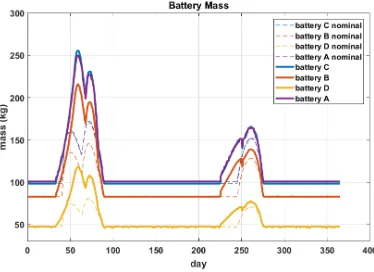
energy requirement is strongly influenced by the uncertainties on the orbits and day 59 is certainly the most affected. From the minmax solution battery D results to be the best one for all the possible mission times. Figure 5 shows that the mass (nominal and maximum) of battery D is the lowest for all days of the year.

Fig. 5. Comparison of the nominal and maximum masses obtained with the four different batteries for each day of 2019.

2) H-Decomposition: The full Belief curve of the battery

sizing problem requires231_{= 2.1475·10}9_{maximisations (one}

the decomposition approach, as explained in Section V-B, is:

N_{F E}DEC =Ns mu

X

i=1

N_{F E,i}u +

mc

X

i=1

N_{F E,i}c = 320 + 2Ns. (30)

Figure 6a shows the partial Belief curve of the mass M

considering all the FEθk,26∈Θ26of the coupled variablesu26

that influence both sub-systems two and six; the other partial curves are not significant for the final reconstruction because, as explained in Section V-B, the uncertainty on the nodes one, three, four and five (and the corresponding orbits) have no influence on the value of the objective function M. Finally Figure 6b shows the reconstructed Belief curve obtained with the h-decomposition approach with five samples in the space of the coupled vectors ui6. Thus, according to (30), 330

different optimisation have been run, strongly reducing the computational cost of the exact evaluation.

For a convergence analysis of the h-decomposition please refer to [3].

(a)

(b)

Fig. 6. Partial Belief curve, Figure 6a, of the coupled vectoru26and Belief

curves, Figure 6b, of the spacecraft’ mass for the day 59 obtained with 5 samples and then 330 optimisations.

D. Validation

A validation of the correctness of the results can be obtained in this way. Decompose the min-max problem in three steps:

• Fix a starting day for the mission:tˆ;

• Maximise the energy requirement over the orbit uncer-tainty:

max

u∈U E(ˆt,a,e,i,Ω,ω,θ)

• Minimise the mass over the design parameters (type of

battery and voltage):

min

d∈D t=ˆt

M(d,a,e,i,Ω,ω,θ,η_b)

with_bη= min(η).

For ˆt = 59 and evaluated argmax_u∈UE (the red curve in Figure 4a, the minimum Mass of the battery (Figure 5) corresponds to battery D and it is 126.3 kg.

VI. CONCLUSION

In this paper we proposed a new approach to optimise complex systems in space systems engineering, affected by epistemic uncertainty. We used Dempster-Shafer theory of Evidence to model uncertainty and Evidence Network Model (ENM) to model the system and its interconnections. From the battery sizing problem one can see that: the proposed constrained min-max scheme produces correct results and the decomposition approach delivers an approximation of the Belief nearly in polynomial time with a low exponent. Future work will include a statistical analysis of the robustness of the constrained minmax algorithm and an accuracy analysis of the approximated Belief curves.

ACKNOWLEDGMENT

This work is partially supported by the ESA NPI grant ref. TEC-ECN-SoW-20140806, ITN UTOPIAE and ESA/ITI project B00016563 Contract No. 4000116741/16NL/MH/GM. The authors gratefully acknowledge the support of Surrey Satellite Technology (SSTL), particularly Kathryn Graham and Kim Birkett, and ESA, particularly Harold Metselaar.

REFERENCES

[1] J. C. Helton Uncertainty and sensitivity analysis in the presence of stochastic and subjective uncertainty, Journal of Statistical Computation and Simulation, 1997, vol. 57, pp. 3–76

[2] W.L. Oberkampf and J.C. Helton, Investigation of Evidence Theory for Engineering Applications, AIAA 2002-1569, 4th Non-Deterministic Approaches Forum, 22-25 April 2002, Denver Colorado.

[3] M. Vasile, G. Filippi, C. Ortega and A. Riccardi, Fast Belief Estimation in Evidence Network Models, EUROGEN 2017.

[4] G. Shafer, A mathematical theory of evidence, Princeton University Press, 1976.

[5] M. VasileOn the Solution of Min-Max Problems in Robust Optimization, The EVOLVE 2014 International Conference, 2014

[6] M. Vasile, E. Minisci and M. Locatelli,An Inflationary Differential Evolution Algorithm for Space Trajectory Optimisation, IEEE Transac-tions on Evolutionary Computation, volume 15, number 2, April 2011. [7] M. Di Carlo, M. Vasile and E. Minisci,Multi-population inflationary differential evolution algorithm with Adaptive Local Restart, IEEE Congress on Evolutionary Computation (CEC), 2015

[8] S. Alicino and M. Vasile, Evidence-based Preliminary Design of Spacecraft, 6th _{International Conference on Systems & Concurrent}

Engineering for Space Applications, October 2014.

[9] M. Vasile,On the Solution of Min-Max Problems in Robust Optimisa-tion, The EVOLVE, 2014.

[10] M. R. Patel,Spacecraft Power Systems, CRC Press, 2005.