Power hardware-in-the-loop setup for developing, analyzing and testing mode identification techniques and dynamic equivalent models

Power Hardware-in-the-Loop Setup for Developing,

Analyzing and Testing Mode Identification

Techniques and Dynamic Equivalent Models

Eleftherios O. Kontis,

Grigoris K. Papagiannis

School of Electrical and Computer Engineering, Aristotle University of Thessaloniki,

Thessaloniki, Greece e-mail: [email protected]

[email protected]

Mazheruddin H. Syed,

Efren Guillo-Sansano,

Graeme M. Burt

and Environment University of Strathclyde,

Glasgow, UK

email: [email protected] [email protected]

[email protected]

Theofilos A. Papadopoulos

Department of Electrical and Computer Engineering, Democritus University of Thrace,

Xanthi, Greece email: [email protected]

Abstract—During the last decades, a significant number of mode identification techniques and dynamic equivalent models have been proposed in the literature to analyze the dynamic properties of transmission grids and active distribution networks (ADNs). The majority of these methods are developed using the measurement-based approach, i.e., by exploiting dynamic responses acquired from phasor measurement units (PMUs). However, there is lack of a common framework in the literature for the performance evaluation of such methods under real field conditions. Aiming to address this gap, in this paper, a power hardware-in-the-loop setup is introduced to generate dynamic responses, suitable for the testing and validation of measurement-based mode identification techniques and dynamic equivalent models. The setup consists of a high voltage transmission grid, two medium voltage distribution grids as well as a low voltage ADN. Using this setup, several disturbances are emulated and the resulting dynamic responses are recorded using PMUs. The measurements are made available to other researchers through a public repository to act as benchmark responses for the evaluation of measurement-based methods.

Index Terms—Active distribution networks, dynamic equiv-alents, inter-area oscillations, system identification techniques, mode identification, power hardware-in-the-loop.

I. INTRODUCTION

With the increased penetration of distributed generation (DG) units into the existing distribution grids, it is becoming more and more complex for power system operators to develop and maintain detailed power system models [1]. To overcome this issue, measurement-based methods have been proposed in the literature to facilitate the dynamic analysis of transmission grids and active distribution networks (ADNs) [2]. In this

The work in this paper has been supported by the European Commission, under the FP7 project ELECTRA (grant no: 609687) and under H2020 project ERIGRID (grant no:654113).

All data underpinning this publication are openly available from the Uni-versity of Strathclyde KnowledgeBase at http://doi.org/10.15129/a1234b56.

context, several measurement-based mode identification tech-niques have been developed to perform on-line modal analysis of transmission and distribution grids [3]–[6]. Additionally, a significant number of reduced order dynamic equivalent models have been proposed to facilitate the dynamic analysis of modern ADNs [7]–[11].

A. Mode Identification Techniques

Mode identification from measured power system responses has drawn great attention in power system industry since the early 1990s [12]. Nowadays, these methods have gained a renewed interest due to the increasing installations of phasor measurement units (PMUs). This renewed interest has also been verified by the recent report of the IEEE Task Force on Identification of Electromechanical Modes [3].

Compared to traditional eigenvalue analysis methods, measurement-based techniques allow the close to real-time estimation of power system modes, thereby enabling novel control and monitoring applications. Using these techniques, wide-area control [13], real-time monitoring of inter-area oscillations [14], prediction of stability margins [3], and fine tuning of power system stabilizers (PSSs) [15] can be under-taken.

B. Reduced Order Dynamic Equivalent models

new and more accurate equivalent models are required to simulate the complex dynamic behavior of these grids. This need is also emphasized by the recent reports of the CIGRE [18] and the IEEE Task Forces [19].

Following this trend, several measurement-based equivalent models have been proposed during the past couple of years to facilitate the dynamic analysis of modern power systems. Using these models, frequency stability analysis [7], small signal and transient stability analysis [8], [9], short- and long-term voltage stability studies [10], as well as fine-tuning of power system model components [20] can be undertaken.

C. Motivation and Scope of the Paper

Generally, the performance of measurement-based mode identification methods and dynamic equivalent models is eval-uated via dynamic responses obtained through simulations, conducted using detailed power system models [6]–[8]. Thus, to evaluate the performance of measurement-based methods, in a systematic and comparative way, benchmark power system models have been developed [21].

Nevertheless, signals obtained through dynamic simulations cannot effectively replicate PMU recordings, which inherently contain noise, outliers and in some cases missing samples [1]. Therefore, the evaluation of measurement-based methods using only simulated responses is not adequate enough, to demonstrate their applicability under real field conditions. For this purpose, actual PMU recordings are required. However, in the literature there is no common framework, i.e. typical sets of dynamic responses recorded through PMUs, to evaluate in a comparative way the accuracy of measurement-based methods. Scope of this paper is to address this gap by generating representative sets of dynamic responses, suitable for testing and analyzing the performance of measurement-based mode identification techniques and dynamic equivalent models. For this purpose, a power hardware-in-the-loop (PHIL) setup is developed, consisting of a modified benchmark high voltage (HV) grid, namely the Kundur two area power system [22]. Two medium voltage (MV) grids, derived using the topology of the European MV distribution grid proposed by CIGRE Task Force C6.04 [23] and a low voltage (LV) ADN which comprises several loads and DG units. The HV and MV grids are simulated in a digital real time simulator (DRTS) from RTDS Technologies, while the Dynamic Power Systems Lab-oratory (DPSL) infrastructure of the University of Strathclyde constitutes the LV ADN. Using the above-mentioned setup, system disturbances are introduced and the dynamic responses of frequency, voltage and current for several system buses are recorded using virtual and hardware PMU devices. The recorded responses are made available to other researchers through a public repository and can be used as benchmark signals for the evaluation of measurement-based models.

The rest of the paper is organized as follows: In Section II the developed PHIL setup is presented and the conducted experiments are discussed in detail. In Section III indicative results are presented. More specifically, the Matrix Pencil method (MP) [3] is used to identify the dominant inter-area

mode of the examined power system, while a reduced order equivalent model, based on the structure proposed in [11], is also developed to simulate the dynamic behavior of a composite load. Finally, Section IV concludes the paper.

II. POWER HARDWARE-IN-THE-LOOP SETUP

A. System Under Study

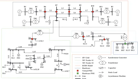
To create a benchmark power system with different voltage levels, a HV transmission grid and two MV distribution grids are implemented on a DRTS. Additionally, a LV ADN is designed using the laboratory infrastructure of the DPSL. The resulting topology is presented in Fig. 1. The HV transmission grid is a modified version of the Kundur two area power system [22], while MV grids are derived by applying mod-ifications on the benchmark European MV distribution grid, developed by the CIGRE Task Force C6.04 [23].

The original Kundur system is a 230 kV, 60 Hz transmis-sion grid, while the CIGRE benchmark MV system is a 20 kV, 50 Hz distribution grid. To achieve an interconnection between the grids, reference values for the control systems of the Kundur two area system are modified and validated to represent 50 Hz conditions. Modeling of transformers (TR1 -TR4), loads (SL1, SL2), capacitors (C1, C2), lines (L1 - L8), synchronous generators (G1 - G4) and the associated control devices, i.e., exciters, governors, and PSSs, is performed using the parameters reported in [22].

To derive the MV distribution grids, the following modi-fications are applied on the benchmark model of [23]. First, the 110/20 kV transformers used in [23] are replaced by two 230/20 kV transformers with on-load-tap-changers (OLTCs), i.e., TR5 and TR6, to allow the coupling with the HV transmission grid. Their parameters are presented in Table I. Furthermore, all switches are considered open, creating two independent radial MV feeders, i.e, MV Feeder #1 and MV Feeder #2. Additionally, to create more complex dynamic responses, several static loads of the model presented in [23] are replaced with induction machines (IMs). A detailed description of all network static loads is presented in Table II, while model parameters for the employed IMs are presented in Table III. Concerning the parameters of distribution lines (L9 - L19), values from [23] are used. Finally, in node N13 of the MV Feeder #2, a 20/0.4 kV OLTC transformer, with data presented in Table I, is considered. This transformer is implemented in the DRTS and used to interconnect the actual LV network of the DPSL with the MV grid.

The actual laboratory environment consists of a 5.5 kVA, 0.87 lagging asynchronous machine (IM6), a 7.5 kVA, 0.87 lagging asynchronous machine (IM7), a static load bank (SL13) as well as an inverter interfaced DG unit (DG1). IM6 operates as motor, while IM7 operates as generator. Both machines operate at 0.8 p.u. The static load bank absorbs 10 kW of real power and 4.84 kVAr of reactive power. The inverter interfaced unit operates under a constant power (P-Q) mode, injecting 8 kW of real power to the grid.

TABLE I

DATA FOR TRANSFORMERSTR5, TR6,ANDTR7 Description Unit Values (TR5 & TR6 / TR7) Transformer ratio (Trat) - 230/20 / 20/0.4

Rated power (Tmva) MVA 25 / 1

Leakage inductance (xl) p.u. 0.08 / 0.04

No load losses (N LL) p.u. 0.001 / 0.001

TABLE II NETWORKSTATICLOADS*

Name Node P(MW) Q(MVAr)

SL1 B7 967.000 100.000

SL2 B9 1767.000 100.000

SL3 N1 19.839 5.703

SL4 N3 0.276 0.069

SL5 N4 0.431 0.108

SL6 N5 0.727 0.182

SL7 N6 0.548 0.137

SL8 N8 0.586 0.147

SL9 N10 0.475 0.119

SL10 N11 0.330 0.083

SL11 N12 20.010 5.797

SL12 N14 0.208 0.052

*All static loads are modeled as constant impedance loads.

TABLE III IM PARAMETERS*

Parameters* IM1 IM2 IM3 IM4 IM5

Node N3 N7 N9 N10 N14

S(MVA) 0.265 0.09 0.675 0.08 0.39

Ra(p.u.) 0.003 0.003 0.004 0.025 0.005 Xa(p.u.) 0.07 0.09 0.09 0.055 0.09

Xmd0(p.u.) 2 3 2.24 1.8 2.2

rf d(p.u.) 0.2 0.5 0.23 0.15 0.3 xf d(p.u.) 0.07 0.042 0.073 0.067 0.08 H (MWs/MVA) 1.5 0.7 1.5 0.93 1.5

*HereSdenotes the rated power of the IM, whileRaandXastator resistance

and leakage reactance, respectively. Xmdo is the unsaturated magnetizing

reactance, whereasrf dandxf dstand for the rotor resistance and reactance,

respectively.H is the machine inertia.

is installed at the LV-Bus. Details concerning the design of the PMU can be found in [24] and [25]. Additionally, using the GTNET-PMU firmware of the DRTS, eight more P class PMUs [26] are represented. These PMUs are assumed to be connected at the HV and MV buses marked with red boxes in Fig. 1. Both the hardware and the software-based PMUs can record the grid frequency as well as positive- and phase-sequence data sets of voltage and current, using a sampling rate equal to 100 samples per second (sps). To time-align data streams and to log the measurements, a custom phasor data concentrator (PDC) was created in programming language C. A short description of the data contained in this PDC is provided in Table IV, while a database containing the raw data

TABLE IV DATASTORED IN THEPDC

PMU Node Voltage Recordings Current Recordings

# 1 B6 Voltages of B6

-# 2 B7 Voltages of B7

-# 3 B8 Voltages of B8

-# 4 B9 Voltages of B9

-# 5 B10 Voltages of B10

-# 6 N1 Voltages of N1

-# 7 N12 Voltages of N12 Currents of TR6 # 8 N14 Voltages of N14 Currents of L20 # 9 LV-Bus Voltages of LV-Bus Currents of TR7

of the experiments can be found in [27].

B. Description of the experiments

Two types of disturbances are considered and investi-gated. The first type includes load connections/disconnections, while the second includes voltage disturbances caused by OLTC actions. As discussed in [4], disturbances caused by load connections/disconnections are ideal for the testing of measurement-based mode identification techniques, while dy-namic responses recorded during OLTC actions are ideal for the parameter estimation of measurement-based equivalent models [28]. The examined sets of disturbances are summa-rized as follows:

• Set-1: Thirteen disturbances are introduced in the HV grid by disconnecting and connecting SL1. In the first disturbance 5% of the load is disconnected. In the second disturbance 10% is disconnected. The same procedure is repeated several times until 75% of the load is disconnected. In all cases, the load is reconnected after 1 s to avoid instability events.

• Set-2: Thirteen disturbances are introduced in the HV grid by disconnecting and connecting SL2. In each disturbance, the power of the disconnected load is increased by 5%. In all cases, the load is reconnected after 1 s.

• Set-3: Four disturbances are introduced in MV Feeder #1, by disconnecting SL3. In the first disturbance, 25% of the load is disconnected. In the rest of the disturbances, the power of the disconnected load is increased by 25% (in the last disturbance the load it totally removed). In all cases, the load is reconnected after 6 s.

• Set-4: Four disturbances are introduced in MV Feeder #2 using SL11. Initially 25% of the load is disconnected and reconnected after 6 s. In every other disturbance, the power of the disconnected load is increased by 25%.

G1

G2

G3

G4 TR1

TR2

TR3

TR4

TR5

B1 B5 B6 B7 B8 B9 B10 B11 B3

B2 B4

L1 L2

L3 L4

L5 L6

L7 L8

SL1 SL2

C1

C2

N1

L19

N14 TR6 _N12

T

R7

SL3

L

9

L10

N2

N3

SL4 IM1

N8

L

11

N4

SL5 N5

L

12

SL6 L13

N6 S2 N7

L

14

SL7 IM2 L15

L16

N

9

IM3

N10

L17 SL9

IM4

L

18

N11

SL10 S3

SL11

N13

SL12 IM5 L20

S1

IM6 IM7 SL13 AC

+ >>>>>> DG1

HV Grid MV Feeder #1 MV Feeder #2 RTDS Model Hardware Virtual PMU Hardware PMU

Synchronous Generator

Asynchonous Machine Transformer

Capacitor

Static Load

Line Node

LV-Bus

SL8

Fig. 1. PHIL setup. HV and MV buses are symbolized using capital letters B and N, respectively. The numbering of HV and MV buses is according to [22] and [23], respectively. Preserving this numbering, the Reader can derive line parameters from [22] and [23].

disturbance, the magnitude of the voltage change is increased by 0.02 p.u.

• Set-6: Voltage disturbances are introduced using the OLTC of transformer TR6. The same procedure as in Set-5 is applied.

• Set-7: Voltage disturbances are introduced using the OLTC of transformer TR7. The same procedure as in Case-5 is adopted.

To provide a further insight on the conducted experiments, the p.u. value of the positive-sequence voltage of HV, MV, and LV grid, is presented in Fig. 2, where indicative recordings from PMUs #1, #6, and #9, are plotted. The base volt-ages are 230 kV, 20 kV, and 0.4 kV, respectively. Each set of disturbances is marked with different dashed lines. As shown, disturbances introduced in the HV grid affect the overall system behavior. Therefore, these events can be used to investigate propagation of inter-area oscillations in both transmission and distribution grids, to test methods aiming to identify inter-area oscillation paths as well as to evaluate the performance of mode identification techniques under ringdown events. On the other hand, disturbances introduced in MV or in LV grids affect only specific parts of the examined power system. For instance, as shown in Fig. 2, during the disturbances of Set-5, the voltages of the HV and LV grid remain practically unaffected. Therefore, these disturbances can be used to develop reduced order equivalent models for specific parts of the examined setup. Additionally, it is worth mentioning that these disturbances result in ambient data (also known as operational data) generation in several system buses. An indicative example is presented in Fig. 2f, where the recordings of PMU #9 during the disturbances of Set-5 are

plotted. Note that Set-5 disturbances are introduced in MV Feeder #1, while PMU #9 is located in the LV ADN, which is connected to MV Feeder #2. The operational data can be used to evaluate the performance of mode identification techniques under ambient conditions as well as to develop equivalent models aiming to analyze the steady-state behavior of the grid.

III. INDICATIVE RESULTS

A. Identification of oscillatory modes

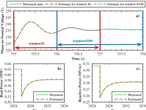
The inter-area mode of the examined power system is identified using data recorded during the last disturbance of Set-1. More specifically, raw data of positive-sequence voltage magnitude, recorded from PMUs #1, #6, and #9, are used. In all cases, the identification procedure is performed successively using the sliding window technique [29]. The first window starts att=755 s. Every other window starts after 0.01 s (relatively to the previous one). All windows contain data for two seconds. Following this approach, 100 windows are created containing data from t=755 s up to t=758 s. For each window, mode frequency f and damping factor σ are estimated using the MP method [3]. In all windows, apart from the inter-area, i.e., oscillatory mode, two surplus exponential modes are added to enhance the accuracy of the identification procedure.

Fig. 2. Positive-sequence voltage recordings. Raw data from a) PMU #1, b) PMU #6, and c) PMU #9. Zooming in the recordings of PMU #9. Data from d) Set-1, e) Set-2, and f) Set-5.

very good agreement between the actual measurement and the estimates is observed, verifying the accuracy of the identifi-cation procedure. In fact, the correspondingR2_{values [9] are}

equal to 99.94 % and 99.39 %, respectively. Similar results are observed for all windows.

B. Development of dynamic equivalent models

In this Subsection, a reduced order dynamic equivalent model is developed to simulate the dynamic behavior of the composite load, connected at N14. For this purpose, voltage and current recordings from PMU #8 are used to calculate the corresponding dynamic responses of real and reactive power. Afterwards, an equivalent model, based on the structure proposed in [11], is developed. The pa-rameters of the model, i.e θp = [α1,p, α2,p, β1,p, β2,p, Tp]

and θq = [α1,q, α2,q, β1,q, β2,q, Tq], are identified based

on the last disturbance of Set-6. Here, θp and θq de-note the sets of parameters used to simulate real and reactive power, respectively (notation according to [11]). The window used for the identification procedure starts at

TABLE V

IDENTIFICATION OFINTER-AREAMODEUSINGRESPONSES FROM

DIFFERENTVOLTAGELEVELS

Parameter HV(PMU #1) MV(PMU #6) LV(PMU #9)

¯

f(Hz) 1.1198 1.0804 1.0788

¯

σ(s−1_{) -1.4211 -1.5236 -1.5139}

t=2825.79 s and ends at t=2836 s. All model parameters are identified through non-linear least square optimization [11]. Initial values for model parameters are derived as dis-cussed in [11]. The optimization results in the following sets: θp = [11.6086,−9.6631,1.8276,−0.8392,1.3255] and

θq = [9.9474,−8.1677,1.8769,−0.8858,1.3703].

The measured and the estimated real and reactive power responses are presented in Figs. 3b and 3c, respectively. As shown, the developed equivalent model simulates very accurately both real and reactive power responses. The R2

755 755.5 756 756.5 757 757.5 758 Time (s)

220 225 230 235 240 245 250

Phase-to-Neutral Voltage (V)

Measured data Estimate for window #1 Estimate for window #100

2824 2828 2832 2836 Time (s)

0.50 0.52 0.54 0.56 0.58 0.60 0.62 0.64

Real Power (MW) Measured

Estimated

2824 2828 2832 2836 Time (s)

0.25 0.26 0.27 0.28 0.29 0.30 0.31

Reactive Power (MVAr)

Measured Estimated

window#100

window#1

a)

b) c)

Fig. 3. a) Mode estimation using the MP method. Indicative results for the first and last window. Derivation of dynamic equivalent model for node N14. Modeling of b) real and c) reactive power.

IV. CONCLUSIONS

In this paper, a PHIL setup is introduced to generate representative sets of dynamic responses, suitable for testing and analyzing the performance of measurement-based mode identification techniques and dynamic equivalent models. The setup consists of a HV grid, two MV grids and a LV ADN. Several disturbances are examined and the resulting dynamic responses are recorded using virtual and hardware PMUs. The recordings are made available to other researches through a public repository.

Additionally, the inter-area mode of the examined setup is identified using the MP method, while a reduced order equivalent model is developed for the composite load, located at N14. In both cases, the identification procedure is presented in detail, while the corresponding results are also listed to act as benchmarks for the performance evaluation of other methods and techniques.

REFERENCES

[1] F. Mahmood, H. Hooshyar, J. Lavenius, A. Bidadfar, P. Lund, and L. Vanfretti, “Real-time reduced steady-state model synthesis of active distribution networks using pmu measurements,” IEEE Trans. Power Del., vol. 32, no. 1, pp. 546–555, Feb. 2017.

[2] U. D. Annakkage, N. K. C. Nair, Y. Liang, A. M. Gole, V. Dinavahi, B. Gustavsen, T. Noda, H. Ghasemi, A. Monti, M. Matar, R. Iravani, and J. A. Martinez, “Dynamic system equivalents: A survey of available techniques,”IEEE Trans. Power Del., vol. 27, no. 1, pp. 411–420, Jan. 2012.

[3] Identification of Electromechanical Modes in Power Systems. IEEE Task Force on Identification of Electromechanical Modes, Technical Report, 2012.

[4] D. J. Trudnowski and J. W. Pierre, “Overview of algorithms for estimating swing modes from measured responses,” in2009 IEEE Power Energy Society General Meeting, Jul. 2009.

[5] J. Thambirajah, E. Barocio, and N. F. Thornhill, “Comparative review of methods for stability monitoring in electrical power systems and vibrating structures,”IET Gen., Trans. Distr., vol. 4, no. 10, pp. 1086– 1103, Oct. 2010.

[6] E. O. Kontis, T. A. Papadopoulos, G. A. Barzegkar-Ntovom, A. I. Chrysochos, and G. K. Papagiannis, “Modal analysis of active distri-bution networks using system identification techniques,” Int. J. Electr. Power Energy Syst., vol. 100, pp. 365–378, Mar. 2018.

[7] H. Golpira, H. Seifi, and M. R. Haghifam, “Dynamic equivalencing of an active distribution network for large-scale power system frequency stability studies,”IET Gen., Trans. Dist, vol. 9, no. 15, pp. 2245–2254, Nov. 2015.

[8] S. M. Zali and J. V. Milanovic, “Generic model of active distribution network for large power system stability studies,”IEEE Trans. Power Syst., vol. 28, no. 3, pp. 3126–3133, Aug. 2013.

[9] E. O. Kontis, S. P. Dimitrakopoulos, A. I. Chrysochos, G. K. Papa-giannis, and T. A. Papadopoulos, “Dynamic equivalencing of active distribution grids,” in2017 IEEE Manchester PowerTech, Jun. 2017. [10] L. Robitzky, D. Mayorga-Gonzalez, C. Kittl, C. Strunck,

J. Zwartscholten, S. C. Muller, U. Hager, J. Myrzik, and C. Rehtanz, “Impact of active distribution networks on voltage stability of electric power systems,” in 2017 IREP Bulk Power Systems Dynamics and Control Symposium, Aug. 2017.

[11] E. O. Kontis, T. A. Papadopoulos, A. I. Chrysochos, and G. K. Papagiannis, “On the applicability of exponential recovery models for the simulation of active distribution networks,”IEEE Trans. Power Del., in press.

[12] J. F. Hauer, C. J. Demeure, and L. L. Scharf, “Initial results in prony analysis of power system response signals,”IEEE Trans. on Power Syst., vol. 5, no. 1, pp. 80–89, Feb. 1990.

[13] N. R. Chaudhuri, A. Domahidi, R. Majumder, B. Chaudhuri, P. Korba, S. Ray, and K. Uhlen, “Wide-area power oscillation damping control in nordic equivalent system,”IET Gen., Transm. Distr., vol. 4, no. 10, pp. 1139–1150, Oct. 2010.

[14] K. Sun, Q. Zhou, and Y. Liu, “A phase locked loop-based approach to real-time modal analysis on synchrophasor measurements,”IEEE Trans. Smart Grid, vol. 5, no. 1, pp. 260–269, Jan. 2014.

[15] Messina and A. Roman,Intear-area Oscillations in Power Systems - A Nonlinear and Nonstationary Perspective. Springer, 2009.

[16] “Load representation for dynamic performance analysis (of power sys-tems),”IEEE Trans. Power Syst., vol. 8, no. 2, pp. 472–482, May 1993. [17] “Standard load models for power flow and dynamic performance simu-lation,”IEEE Trans. Power Syst., vol. 10, no. 3, pp. 1302–1313, Aug. 1995.

[18] Modelling and Aggregation of Loads in Flexible Power Networks. Cigre Working Group C4.605, Technical Report, 2014.

[19] Contribution to Bulk System Control and Stability by Distributed Energy Resources Connected at Distribution Network. IEEE Task Force on Contribution to Bulk System Control and Stability by Distributed Energy Resources Connected at Distribution Network, Technical Report, 2017. [20] Power System Model Validation. NERC Model Validation Task Force,

Technical Report, 2010.

[21] P. Demetriou, M. Asprou, J. Quiros-Tortos, and E. Kyriakides, “Dynamic ieee test systems for transient analysis,”IEEE Systems Journal, vol. 11, no. 4, pp. 2108–2117, Dec. 2017.

[22] P. Kundur,Power System Stability and Control. McGraw-Hill, 1994. [23] Benchmark Systems for Network Integration of Renewable and

Dis-tributed Energy Resources. Cigre Task Force C6.04, Technical Report, 2014.

[24] A. J. Roscoe, I. F. Abdulhadi, and G. M. Burt, “P and m class phasor measurement unit algorithms using adaptive cascaded filters,” IEEE Trans. Power Del., vol. 28, no. 3, pp. 1447–1459, Jul. 2013.

[25] A. J. Roscoe and S. M. Blair, “Choice and properties of adaptive and tunable digital boxcar (moving average) filters for power systems and other signal processing applications,” inIEEE International Workshop on Applied Measurements for Power Systems (AMPS), Sept. 2016. [26] IEEE Standard for Synchrophasor Measurements for Power Ssystems,

IEEE, C37.118.1-2011, 2011. [27] http://doi.org/10.15129/a1234b56.

[28] D. Karlsson and D. J. Hill, “Modelling and identification of nonlinear dynamic loads in power systems,”IEEE Trans. Power Syst., vol. 9, no. 1, pp. 157–166, Feb. 1994.