On-Orbit Manoeuvring Using Superquadric Potential Fields

(1)

UNIVERSITY OF STRATHCLYDE

Department of Mechanical Engineering

ON-ORBIT MANOEUVRING USING SUPERQUADRIC

POTENTIAL FIELDS

Ahmed Badawy B.Sc., M.Sc.

A thesis presented in fulfilment to the requirements for the

degree of

D

OCTOR OF

P

HILOSOPHY

(2)

The copyright of this thesis belongs to the author under the terms of the United

Kingdom Copyright Acts as qualified by University of Strathclyde Regulation 3.49.

Due acknowledgement must always be made of the use of any material contained in,

(3)

ACKNOWLEDGEMENT

This research could not have been conducted without help and

support of my parents who despite being away in Egypt, always

encourage me to complete this thesis as best as I can. So whatever I

express, my gratitude toward them, it is really less than what they

deserve.

I also wish to express my appreciation to my wife who left her parents

to be with me during these busy years. She was the one who suffered a

lot to help me conduct this research. Although she is yet to know what

is going around, my daughter plays a wonderful role in relieving

stresses accompanying this hard time.

A special appreciation and thanks to

who gave me a

wonderful example of cooperation and guidance throughout the

research. He devoted a lot of time and effort in discussion, revision,

and stimulating suggestions that greatly enhanced my scientific

knowledge.

A real help and support were offered by the Department of

Mechanical Engineering at the University of Strathclyde. Everyone

did their utmost to help and offer an ideal research environment for

researchers.

(4)

ABSTRACT

Onorbit manoeuvring represents an essential process in many space missions such

as orbital assembly, servicing and reconfiguration. A new methodology, based on

the potential field method along with superquadric repulsive potentials, is discussed

in this thesis. The methodology allows motion in a cluttered environment by

combining translation and rotation in order to avoid collisions. This combination

reduces the manoeuvring cost and duration, while allowing collision avoidance

through combinations of rotation and translation.

Different attractive potential fields are discussed: parabolic, conic, and a new

hyperbolic potential. The superquadric model is used to represent the repulsive

potential with several enhancements. These enhancements are: accuracy of

separation distance estimation, modifying the model to be suitable for moving

obstacles, and adding the effect of obstacle rotation through quaternions.

Adding dynamic parameters such as object translational velocity and angular

velocity to the potential field can lead to unbounded actuator control force. This

problem is overcome in this thesis through combining parabolic and conic functions

to form an attractive potential or through using a hyperbolic function. The global

stability and convergence of the solution is guaranteed through the appropriate

choice of the control laws based on Lyapunov's theorem.

Several onorbit manoeuvring problems are then conducted such as onorbit

assembly using impulsive and continuous strategies, structure disassembly and

reconfiguration and freeflyer manoeuvring near a space station. Such examples

demonstrate the accuracy and robustness of the method for onorbit motion

(5)

1. INTRODUCTION

1

1.1 Background 1

1.2 Motion Planning Classification 3

1.3 Configuration Space 5

1.4 Motion Planning Methods 6

1.4.1 Skeleton (Roadmap) 6

1.4.2 Cell decomposition 8

1.4.3 Other methods 9

1.5 Potential Field Methods 9

1.5.1 Force involving artificial repulsion (FIRAS) 12

1.5.2 Gaussian function 13

1.5.3 Power law function 15

1.5.4 Superquadric functions 16

1.5.5 Harmonic potential functions 17

1.5.6 Navigation functions 17

1.5.7 Fuzzy potential 18

1.6 Thesis Objectives 18

1.7 Thesis Organization 19

(6)

2. ATTRACTIVE POTENTIAL FUNCTIONS

22

2.1 Introduction 22

2.2 Lyapunov’s Stability Theorem 23

2.2.1 Definitions: 24

2.2.2 Lyapunov's second theorem 24

2.3 Translational Attractive Potential 25

2.3.1 Parabolicwell 26

2.3.2 Conicwell 28

2.3.3 Parabolicwell attractive potential with velocity term 29

2.3.4 Conicwell attractive potential with velocity term 30

2.3.5 Hyperbolic attractive potential 30

2.3.6 Hyperbolic attractive potential with velocity term 32

2.4 Rotational Attractive Potential 32

2.4.1 Orientation definition 32

2.4.2 Rotational potential function 34

2.4.3 Rotational potential function with angular velocity term 35

2.5 Global Attractive Potential 38

2.5.1 Example I 38

2.5.2 Example II 44

2.6 Conclusions 49

3. SUPERQUADRIC OBSTACLE REPRESENTATION

50

3.2 Inside-Outside Function 52

3.3 Superquadrics and Motion Planning 53

3.4 Separation Distance 54

3.4.1 Approximate Euclidian distance 54

3.4.2 Pseudodistance 55

(7)

3.4.4 Rigid Body Radial Euclidian distance 57

3.5 Attitude-Distance Effect 59

3.6 Superquadric Obstacle Representation 61

3.6.1 Parallelepiped shape (cuboid) 61

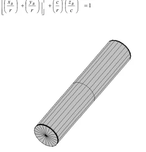
3.6.2 Cylindrical obstacle (beam) 67

4. SUPERQUADRIC OBSTACLE POTENTIAL

73

4.2 Types of Obstacle Potential 73

4.2.1 Avoidance potential 74

4.2.2 Approach potential 74

4.3 Obstacle Potential of Parallelepiped Element 78

4.3.1 Cuboid obstacle potential using the modified pseudo distance 78

4.3.2 Cuboid obstacle potential using the rigid body radial Euclidian distance 81

4.4 Obstacle Potential of a Cylindrical Element 85

5. GLOBAL POTENTIAL FUNCTION

88

5.2 Continuous Control 89

5.3 Impulsive Control 96

5.4 Conclusions 103

6. ORBITAL ASSEMBLY

105

6.1 Introduction 105

6.2 Proximity Motion 106

(8)

6.4 On-Orbit Continuous Control 112

6.4.1 Continuous assembly using conic and parabolic potentials 112

6.4.2 Continuous assembly using hyperbolic potential 122

6.5 On-Orbit Impulsive Control 127

6.5.1 Example I 128

6.5.2 Example II 136

6.5.3 Complex structure assembly 139

7. ORBITAL RECONFIGURATION

148

7.1 Introduction 148

7.2 Free Flyer Manoeuvring Near a Space Station 149

7.3 Structure Reconfiguration 154

8. CONCLUSIONS

174

8.1 Review 174

8.2 Future Work 177

References 179

Appendix A: Quaternion Algebra

188

A.1 Introduction 188

(9)

LIST OF FIGURES

Fig. 1.1 Space exploration rovers 2

Fig. 1.2 Motion planning phases 2

Fig. 1.3 Motion planning levels of complexity 4

Fig. 1.4 Three link mechanism 5

Fig. 1.5 The visibility graph 7

Fig. 1.6 The Voronoi diagram 8

Fig. 1.7.a) Global potential with FIRAS rectangular obstacle representation 12

Fig. 1.7.b) Global potential with FIRAS circular obstacle representation 13

Fig. 1.8 Global potential with Gaussian obstacle representation 14

Fig. 1.9 Global potential with power law obstacle representation, N = 10 15

Fig. 1.10 Global potential with superquadric obstacle representation 16

Fig. 1.11 Thesis roadmap 20

Fig 2.1 Parabolicwell attractive potential 27

Fig 2.2 Conicwell attractive potential 28

Fig 2.3 Hyperbolicwell attractive potential 31

Fig. 2.4 Manoeuvring object motion in 3D 40

Fig. 2.5.a) Manoeuvring object total impulses 40

Fig. 2.5.b) Manoeuvring object impulses in the xdirection 41

Fig. 2.5.c) Manoeuvring object impulses in the ydirection 41

Fig. 2.5.d) Manoeuvring object impulses in the zdirection 42

Fig. 2.6.a) Manoeuvring object error quaternion 42

Fig. 2.6.b) Manoeuvring object angular velocities 43

Fig. 2.6.c) Manoeuvring object torques 43

Fig. 2.7 Manoeuvring object motion in 3D 45

Fig. 2.8.a) Manoeuvring object velocity 46

Fig. 2.8.b) Manoeuvring object acceleration 46

Fig. 2.9.a) Manoeuvring object error quaternions 47

Fig. 2.9.b) Manoeuvring object angular velocity 47

Fig. 2.9.c) Manoeuvring object angular acceleration 48

Fig. 2.9.d) Manoeuvring object control torque 48

(10)

Fig. 3.2 Superquadric shapes 52

Fig. 3.3 Radial Euclidian distance 57

Fig. 3.4 Possible collision configuration 58

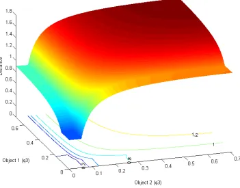
Fig. 3.5 Orientation effect on separation distance 59

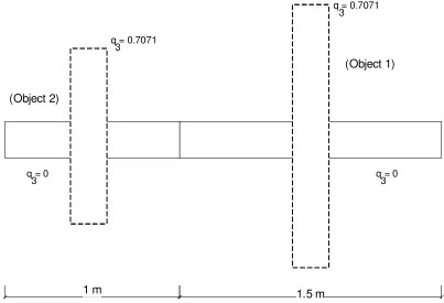
Fig. 3.6 Two object configuration 60

Fig. 3.7 Separation distance vs. quaternion parameter about zaxis 61

Fig. 3.8 Cuboid element representation using a superquadric function 63

Fig 3.9.a) Cuboid isodistance contours, modified pseudo distance method, Eq.

(3.7), ( = 1) 64

Fig. 3.9.b) Cuboid isodistance contours, modified pseudo distance method ( =

100) 64

Fig. 3.9.c) Cuboid isodistance contours radial distance method, Eq. (3.12), ( = 1)

65

Fig. 3.9.d) Cuboid isodistance contours radial distance method ( = 100) 65

Fig. 3.9.e) Cuboid isodistance contours, rigid body radial distance method, Eq.

(3.16), ( = 1) 66

Fig. 3.9.f) Cuboid isodistance contours, rigid body radial distance method ( =100)

66

Fig. 3.10 Cylindrical element representation using a superquadric function 67

Fig. 3.11.a) Beam isopotential contours, pseudo distance method, Eq. (3.7), (cross

section) 68

Fig. 3.11.b) Beam isopotential contours, pseudo distance method (longitudinal

section) 69

Fig. 3.11.c) Beam isodistance contours, radial distance method, Eq. (3.12), (cross

section) 69

Fig. 3.11.d) Beam isodistance contours, radial distance method (longitudinal

section) 70

Fig. 3.11.e) Beam isodistance contours, radial distance for rigid body method, Eq.

(3.16), (cross section) 70

Fig. 3.11.f) Beam isodistance contours, radial distance for rigid body method

(longitudinal section) 71

(11)

Fig. 4.1.b) Avoidance potential function ( = 10) 76

Fig. 4.1.c) Approach potential function ( = 1) 76

Fig. 4.1.d) Approach potential function ( = 10) 77

Fig. 4.2 Radial Euclidian distance 82

Fig. 5.1 Initial configuration 91

Fig. 5.2.a) Object configuration at t = 70 sec 91

Fig. 5.2.b) Object configuration at t = 93 sec 92

Fig. 5.2.c) Final object configuration at t = 130 sec 92

Fig. 5.3 Object trajectories 93

Fig 5.4.a) Object velocities in xdirection 93

Fig 5.4.b) Object velocities in zdirection 94

Fig 5.4.c) Object accelerations in xdirection 94

Fig 5.4.d) Object accelerations in zdirection 95

Fig 5.5.a) Object angular velocities about yaxis 95

Fig 5.5.b) Object angular accelerations about yaxis 96

Fig. 5.6 Initial object configuration 98

Fig. 5.7.a) Object configuration at t = 165 sec 98

Fig. 5.7.c) Object configuration at t = 310 sec 99

Fig. 5.7.d) Final object configuration at t = 1000 sec 100

Fig. 5.8 Object trajectories 100

Fig. 5.9.a) Object impulses in xdirection 101

Fig. 5.9.b) Object impulses in zdirection 101

Fig. 5.10.a) Object error quaternion about yaxis 102

Fig. 5.10.b) Object angular velocities about yaxis 102

Fig. 5.10.c) Object torques about yaxis 103

Fig. 6.1 Inertial, local orbiting and body frames for the ith manoeuvring object 107

Fig. 6.3.a) Object configuration t = 124 sec 114

Fig. 6.3.b) Object configuration t= 838 sec 114

Fig. 6.3.c) Object configuration t = 3470 sec 115

(12)

Fig. 6.4.a) Object velocities in the xdirection 116

Fig. 6.4.b) Object accelerations in the xdirection 116

Fig. 6.4.c) Object velocities in the ydirection 117

Fig. 6.4.d) Object accelerations in the ydirection 117

Fig. 6.4.e) Object velocities in the zdirection 118

Fig. 6.4.f) Object accelerations in the zdirection 118

Fig. 6.5.a) Error quaternions of Objects 1, 3, 9, and 11 119

Fig. 6.5.b) Angular velocity about xaxis of objects 1, 3, 9, and 11 119

Fig. 6.5.c) Error quaternions of objects 5, 6, 7, and 8 120

Fig. 6.5.d) Angular velocity about zaxis of objects 5, 6, 7, and 8 120

Fig. 6.5.e) Torque about xaxis of objects 1, 3, 9, and 11 121

Fig. 6.5.f) Torque about zaxis of objects 5, 6, 7, and 8 121

Fig. 6.7.a) Object configuration (t = 37 sec) 124

Fig. 6.7.b) Object configuration (t = 120 sec) 124

Fig. 6.7.c) Object configuration (t = 180 sec) 125

Fig. 6.7.d) Final object configuration (t = 300 sec) 125

Fig. 6.8.a) Object velocities in xdirection 126

Fig. 6.8.b) Object velocities in zdirection 126

Fig. 6.8.c) Object angular velocities about yaxis 127

Fig. 6.9.a) Initial object configuration 129

Fig. 6.9.d) Object configuration at t = 8300 sec 131

Fig. 6.9.e) Object configuration at t = 8900 sec 131

Fig. 6.9.f) Assembled structure at t = 9800 sec 132

Fig. 6.10.a) Object trajectories 132

Fig. 6.10.b) Object error quaternions 133

Fig. 6.10.c) Object angular velocities 133

Fig. 6.11.a) Impulse in the xdirection (object 7) 134

Fig. 6.11.b) Impulse in the zdirection (object 7) 134

(13)

Fig. 6.11.d) Rate of change of the overall potential (object 7) 135

Fig. 6.12.a) Object trajectories 136

Fig. 6.12.b) Impulses in the xdirection (object 7) 137

Fig. 6.12.c) Impulses in the zdirection (object 7) 137

Fig. 6.12.d) Overall potential (object 7) 138

Fig. 6.12.e) Rate of change of the overall potential (object 7) 138

Fig. 6.13.d) Object configuration at t = 2670 sec 141

Fig. 6.13.e) Object configuration at t = 3725 sec 141

Fig. 6.13.f) Assembled structure at t = 4000 sec 142

Fig. 6.14.a) Object trajectories (object 1 to 7) 142

Fig. 6.14.b) Plate element trajectories (object 15 and 16) 143

Fig. 6.14.c) Impulse in xdirection (object 1) 143

Fig. 6.14.d) Impulse in ydirection (object 1) 144

Fig. 6.14.e) Impulse in zdirection (object 1) 144

Fig. 6.15.a) Error quaternions about the xaxis 145

Fig. 6.15.b) Error quaternions about the yaxis 145

Fig. 6.15.c) Error quaternions about the zaxis 146

Fig. 6.15.d) Continuous control torque about the yaxis 146

Fig. 7.1 International space station using superquadric model 149

Fig. 7.2 Freeflyer trajectory 152

Fig. 7.3 Freeflyer rotation 152

Fig. 7.4.a) Freeflyer thrust impulses in xdirection 153

Fig. 7.4.b) Freeflyer thrust impulses in zdirection 153

Fig. 7.5 Required control torque about yaxis 154

Fig. 7.6.d) Object configuration (t = 145 sec) 157

(14)

Fig. 7.6.f) Object configuration (t = 260 sec) 158

Fig. 7.6.g) Final configuration (t = 400 sec) 158

Fig. 7.7.a) Impulse in the xdirection 159

Fig. 7.7.b) Impulse in the ydirection 159

Fig. 7.7.c) Impulse in the zdirection 160

Fig. 7.8.a) Error quaternions about the xaxis 160

Fig. 7.8.b) Error quaternions about the yaxis 161

Fig. 7.8.c) Error quaternions about the zaxis 161

Fig. 7.8.d) Angular velocity about the xaxis 162

Fig. 7.8.e) Angular velocity about the yaxis 162

Fig. 7.8.f) Angular velocity about the zaxis 163

Fig. 7.9.a) Control torque about the xaxis 163

Fig. 7.9.b) Control torque about the yaxis 164

Fig. 7.9.c) Control torque about the zaxis 164

Fig. 7.10.a) Object configuration (t = 15 sec) 165

Fig. 7.10.d) Object configuration (t = 200 sec) 167

Fig. 7.11.a) Impulse in the x-direction 167

Fig. 7.11.b) Impulse in the y-direction 168

Fig. 7.11.c) Impulse in the z-direction 168

Fig. 7.12.a) Error quaternion about the x-axis 169

Fig. 7.12.b) Error quaternion about the y-axis 169

Fig. 7.12.c) Error quaternion about the z-axis 170

Fig. 7.12.d) Angular velocity about the x-axis 170

Fig. 7.12.e) Angular velocity about the y-axis 171

Fig. 7.12.f) Angular velocity about the z-axis 171

Fig. 7.13.a) Control torque about the xaxis 172

Fig. 7.13.b) Control torque about the yaxis 172

(15)

LIST OF TABLES

Table 5.1 Element translation cost 103

Table 7.1 First phase translation cost 155

(16)

1. INTRODUCTION

1.1 Background

Mobile robots and manipulators are widely used for terrestrial, subsea, and space

applications. Terrestrial applications are vast, ranging from industrial to domestic

usage (Palacín et al., 2004). In industrial applications, combinations of mobile

robots and manipulators serve for mechanical assembly (Yuan, 2002), material

handling (Neuhaus and Kazerooni, 2001), and spot welding (Pires and Loureiro,

2003). Medical robot applications are a further success (and challenge) assisting

during microsurgeries and rehabilitation (Salcudean et al., 1999; Cepolina and

Michelini, 2004). Mobile robots also play a role in subsea and ocean operations

where they are able to reach extreme depth and perform assembly and maintenance

tasks (Antonelli et al., 2001). Well known space applications serve for assembly,

service, and repair (McQuade and McInnes, 1997; Roger, 2003). Other robotic

applications are in rough terrain such as mining and rescue (Lagnemma and

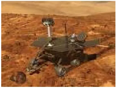
Dubowsky, 2004; Shimoda et al., 2005). Planetary exploration such as Lunar and

Mars rovers, Fig. 1.1, are well known applications which require highly automated,

unattended robotic motion planning (Hayati et al., 1996). Challenges for such

applications have been discussed (Weisbin et al., 1999; Schenker et al., 2000).

As robots are used to perform certain tasks they always require motion; motion is

an essential action without which a robot will lose its functionality. Since robots are

not the sole object in their workspace, robot motion planning research is a key area

of robot technology. Intelligent motion planning (MP) algorithms attempt to

advance from repetitive preprogrammed tasks to fully autonomous operations.

Research development has been undertaken in theory, computational capabilities

and sensors. Determining a collisionfree path between some start and goal

configuration, in addition to the required dynamic parameters, forces and moments,

(17)

[image:17.595.335.526.56.203.2]

(a) ESA EXOMARS Rover (b) NASA Mars Exploration Rover (MER)

Fig. 1.1 Space exploration rovers

Various aspects of MP problems have been investigated either through theoretical

or experimental analysis. Generally, the MP problem aims to find if a region of

space is reachable from another through a continuous path. It is therefore the process

of selecting a path and the associated set of input forces and torques from the set of

all possible motions and inputs, while ensuring that all constraints are satisfied.

Three closely linked problems constitute MP: path planning, trajectory planning,

and motion control, Fig. 1.2. The first phase aims to define the kinematic

parameters, position and orientation, of the manoeuvring object, whereas the second

phase aims to generate the required translational velocity and angular velocity

profile to generate motion to the goal. Path planning is therefore a subset of

trajectory planning. Finally, the motion control phase aims to drive the manoeuvring

object to follow the reference trajectory as closely as possible.

Path

Planning

Trajectory

Planning

Motion

Control

(18)

1.2 Motion Planning Classification

MP algorithms depend on the availability of sensed data such as obstacle shapes

and kinematics. MP methods based mainly on sensed data are normally termed local

methods, used when there is not enough global data about the workspace. Socalled

global methods are used otherwise, when complete knowledge of the workspace is

available. It is also possible to utilize local methods in the case of a well known

environment with either stationary or moving obstacles, but with an optimized path.

A combination of global and local methods can be used to generate a global optimal

plan, with the local sensory based approach reaching to unforeseen obstacles.

Ensuring global knowledge of the workspace is not simple due to limited sensing

capabilities and sensor range limitations. On the other hand, local MP may lead to

unfeasible trajectories as a complete world model is not available. Information

exchange between different manoeuvring objects through decentralized control

enhances the amount of world information available to each of them.

A second classification of MP depends on the obstacle kinematic properties, either

static or dynamic. In the static case, all obstacles are known as in case of robotic

assembly in a production process. On the other hand, in dynamic MP problems the

manoeuvring objects sense data whilst in motion. Consequently, new data is

continuously generated so online control is required. Generally, dynamic MP is the

norm whereas static MP is an exception as every MP problem can be solved as

dynamic one, while the inverse is not true.

Other issues in MP problems occur when dealing with articulated or linked bodies

or deformable problems, where objects shapes will change during motion. These

deformable MP problems are common as a wide range of robots are equipped with

manipulators or links. The level of complexity of MP problems with respect to

objects representations, object dynamic properties, the type of manoeuvring object

under control, and constraint types is illustrated in Fig. 1.3.

Objects in the environment can be represented as spherical shapes for simplicity,

although the real shape is required in cases where the spherical shape occupies

significantly more space than its actual size, or in case of the final docking phase

(19)

Poin

t Mass

S

ing

le Bo

dy

Multi

p

le Point Masses

Multiple Bodies Deformable Bodies

No

nh

olo

n

o

m

ic

Holonomic

Fig. 1.3 Motion planning levels of complexity

Manoeuvring objects range from point mass robots to deformable or articulated

ones. The more degrees of freedom (DOF) associated with manoeuvring objects, the

greater the complexity of the MP problem. Object dynamic properties have a large

influence on the degree of complexity of MP problem. Static objects are much easier

to handle as their positions are known, whereas moving objects add more variables

to the MP problem. Finally, the types of constraints, holonomic or nonholonomic,

affect the number of DOF required to represent the system. Holonomic constraints

reduce the number of DOF associates with the obstacles, whereas nonholonomic

constraints that depend on velocity and position do not affect the number of DOF

(Latombe, 1991). Lastly, bounded forces and torques are required and affect the

choice of MP algorithm as real actuators can saturate.

A general review of MP algorithms is discussed in the following sections. Motion

planning problem is solved within different spaces such as the Cartesian (physical or

task) space or configuration space. Motion parameters in the Cartesian space are

(20)

angles, direction cosines, or quaternions. Since the rest of the thesis deals with

Cartesian spaces, a brief discussion of the configuration space is introduced in the

following section.

1.3 Configuration Space

Like real physical space, Configuration space (CSpace) is defined by a set of

independent parameters or generalized coordinates, which describe the position of

every point on the manoeuvring object at any time based on classical mechanics. For

a point robot in three dimensions, the CSpace is identical to the physical space with

the same number of DOF in ℜ3 _{, while for}_N_{point robots the configuration space is}

ℜ3N

. A rigid rod in 2D, for example, requires three parameters to represent the

CSpace: two coordinates for the position of a reference point, which could be any

point on the rod, and one angle representing the rod orientation about a

perpendicular axis.

As an example of a three link mechanism, Figure 1.4 shows a possible set of

generalized coordinates 1, 2 and 3. Each configuration in the workspace

corresponds to a point in the Cspace. Moreover, the motion of an articulated body

appears as a curve in the CSpace. After generation of the CSpace, all MP problems

are essentially identical.

(21)

Representing points of both manoeuvring objects and obstacles in CSpace

determines whether collisions will occur. If any manoeuvring object point in C

Space lies inside any obstacle or any other manoeuvring object, then collision will

occur. Furthermore, another case occurs when a point of any manoeuvring object

lies on the boundary of any other object, so that smooth contact will occur. Many

computational methods are able to search for CSpace collisions (Branicky and

Newman, 1990; Hwang and Ahuja, 1992).

1.4 Motion Planning Methods

Large numbers of methods exist to solve the MP problem. However a few key

methods are defined: skeleton, cell decomposition, potential field, mathematical

programming, and boundary following methods. Designing a high performance

motion planner usually requires the utilization of more than one MP approach such

as combining the potential field method along with the cell decomposition method

(Chiou et al., 1999). A brief discussion of key methods is provided before going on

to discuss the potential field method. These approaches are either complete or

incomplete. Completeness is defined as finding a path if it is exist, otherwise

returning a failure. Incomplete approaches may terminate in a position other than the

goal, such as a local minimum, but nevertheless the path exists. Complete

algorithms may fail to find a solution if the resolution of the algorithm is not good

enough to find a free path (Goldberg, 1994).

1.4.1 Skeleton (Roadmap)

All possible configurations are retracted into a network of onedimensional lines,

the roadmap, limiting the MP problem to graphsearching. Various methods are

constructed which depend on this basic idea. For 2D problems, the visibility graph

and the Voronoi diagram are commonly used.

The visibility graph, which is one of the earliest roadmap methods, was suggested

by Nilsson (Nilsson, 1969) as a collection of lines connecting all polygonal obstacles

(22)

shortest path will then be chosen as the optimum one between the start and goal

point, as shown in Fig. 1.5.

The Voronoi diagram is used when it is required to maintain some distance

between the manoeuvring object and obstacles. Constructing a Voronoi diagram is

done through defining a set of points called nodes. These nodes are the intersecting

points of equidistant contour lines surrounding the obstacles. The Voronoi diagram

divides the space into regions with only one edge or polygon inside, as shown in

Fig. 1.6.

More complexity arises when dealing with 3D MP problems using the visibility

graph or the Voronoi diagram. A general method of constructing a skeleton in higher

dimensions is constructed through a process called Silhouette. This process is based

on projecting an object from a higher dimensional space to a lower one, and then

tracing the boundaries. This operation could be repeated reaching a set of one

dimensional lines. A simpler Voronoi diagram for 3D objects has been discussed

(Dattasharma and Keerthi, 1995). After generating enough free configurations, the

roadmap is built by connecting them. This is a very efficient MP approach,

especially when high number of DOF exist (Kavraki and Latombe, 1998).

Start

Goal

Obstacle

(23)

Goal

Start

Obstacle

Fig. 1.6 The Voronoi diagram

The roadmap method has also been adapted to dynamic environments of both free

flying and articulated robots (Van den Berg and Overmars, 2005). A possible

combination of the visibility graph and the Voronoi diagram is achieved through

introducing the visibility graph into the Voronoi diagram (Wein et al., 2007).

1.4.2 Cell decomposition

In this method, the free CSpace is decomposed into simple adjacent regions,

called cells. A free path connecting start and goal points is obtained through

connecting the start and goal cells with continuous free cells, called a connectivity

graph. Two ways are used to perform cell decomposition: exact and approximate

cell decomposition.

Exact cell decomposition, object dependent, uses obstacles boundaries to form the

cells whose union is the free space. This produces a smaller number of cells with

(24)

In approximate cell decomposition, object independent, methods a small, simple

cell is chosen then tested whether it is a free cell or belongs to the configuration

obstacles. The free space representation is strictly inclusive in the union of these

small cells, however it does not represent the whole free space since the cells do not

tightly enclose obstacles. Some cells may contain both free space and configuration

obstacles; hence they could not be used to find a path (Brooks and LozanoPérez,

1982).

Cells lying entirely in the free space are used to construct the connectivity graph. If

no connectivity graph is found, higher cell decomposition resolution might be a

solution otherwise no free path exists between the initial and goal configurations

(Latombe, 1991). Approximate methods are used initially to solve the MP problem,

refining until a solution is found or no path is obtained. Cell decomposition is

guaranteed to find a free path if exists, otherwise the algorithm returns failure.

1.4.3 Other methods

Other methods are defined such as: mathematical programming and boundary

following methods. In mathematical programming, the free space is defined as a set

of inequalities, then an optimum curve connecting the start and the goal position is

found. Nonlinear programming is used to solve the motion planning problem by

minimizing path length subject to constraints (Henrich, 1997).

The objective of the boundary following method is to command the manoeuvring

object to move toward its goal in a straight line. In case of being obstructed by an

obstacle, the manoeuvring object traces the obstacle edges. This approach is adapted

to work with a scene filled with unknown obstacles of arbitrary shape and size. Data

about the environment are collected online with sensors (Lumelsky and Stepanov,

1987).

1.5 Potential Field Methods

Many physical systems relax their configuration to attain the lowest possible

energy state. This idea has been adopted and used in the motion planning algorithms

(25)

Each location in the workspace has some scalar potential associated with it. The

potential depends on the relative position between both goal and obstacles positions,

and the manoeuvring object. A virtual attractive potential field representing a goal

and virtual repulsive potential field representing obstacles are merged together to

generate a global potential field, the gradient of which in principle provides a

collisionfree path to the goal. The method is widely used for autonomous mobile

robot path planning in fixed workspaces where both target and obstacles are

stationary. The method is also adapted to deal with moving obstacles (Tzafestas et

al., 2002) and moving goal points through defining a potential function that is

velocity dependent (Ge and Cui, 2002). The method is defined over both the

Cartesian space and the configuration space (Barraquand et al., 1991). However,

limitations of this simple and elegant approach arise when the superposition of the

repulsive potential and attractive potential creates local minima. In addition motion

oscillation in the presence of obstacles and in narrow passages, and the problem of

trapping between two close obstacles also arise (Koren and Borenstein, 1991).

Another advantage of the potential field method appears in its unified approach to

fulfil the MP problem, unlike other methods which divide it as seen in Fig. 1.1. The

outputs of this method are geometrical, dynamical, and lead directly to a control law.

A detailed description of this method is introduced in the subsequent sections as the

rest of the thesis is implemented using the potential field method.

As the number of DOF increases, an exact solution of MP problem is ineffective

(Sharir, 1997). When choosing potential field methods (PFM) to perform the MP

process, an important question should be answered. Which PFM is most suitable for

the current MP problem? The answer to this question is not a matter of choice, it

mainly depends on the manoeuvring object, workspace, computational capabilities,

convergence requirements and obstacle dynamic properties.

During the past three decades, many PFMs have been investigated. Some suggest

how to represent obstacles; others define how to generate both attractive and

repulsive potentials. The two main types of MP problems, global and local, both

utilize potential field functions. The majority of the potential field methods use a

local path planner such as: force involving artificial repulsion (FIRAS), Gaussian

(26)

and Ahuja, 1998), whereas harmonic potential functions and the navigation function

are considered as global path planners. In local path planning, potential functions,

both attractive and repulsive, are formed separately then added to form the global

potential. This has online capability since no prior information about the workspace

is required and the information is gathered whilst in motion. For global path

planning potential functions all information about the workspace should be available

from the start of the process, hence optimized paths can be obtained if these exist

without local minima formation.

Other techniques such as the vector potential field and sliding mode theory are

used. The vector potential field produces a smooth and bounded control. It can

provide better performance compared to scalar field (Masoud and Bayoumi, 1993;

Masoud and Masoud, 2000). Sliding mode theory is used with the potential field

function to perform fast manoeuvres (Jan and Chiou, 2003).

The potential field method has also been developed for space applications in areas

such as proximity manoeuvring (Roger and McInnes, 2000), large angle slew

manoeuvres (McInnes, 1994; McInnes, 1995; McInnes, 1996; Radice and McInnes,

1999; Wisniewski and Kulczycki, 2005), formationflying (McQuade et al., 2003;

Avanzini et al., 2005a; Avanzini et al., 2005b), and autonomous and distributed

motion planning for satellite swarms (Izzo and Pettazzi, 2005; Izzo and Pettazi,

2007). Other work has focused on the assembly of large, complex space structures

using extensions of the potential field methodology (Badawy and McInnes, 2006c;

Badawy and McInnes, 2006b; Badawy and McInnes, 2007c). Here the adjacency

matrix of the graph of the final structure is used to form a global potential field

(McQuade and McInnes, 1998). The structure can then be reconfigured by

modifying the adjacency matrix as required. A related approach has been used for

the autonomous assembly of a group of homogeneous components by defining and

summing vector fields which capture sets of behaviours. The final configuration of

the system is defined by the equilibrium state of the dynamical system formed by the

vector fields, in a similar manner to the global minimum of an artificial potential

(27)

1.5.1 Force involving artificial repulsion (FIRAS)

A region of obstacle influence is chosen for symmetrical obstacles, d_min, beyond

which no effect of the obstacle potential occurs. A continuous differentiable function

for obstacle potential is defined as:

⎧₁ _⎛₁ ₁ _⎞2

V_obs=⎪_⎨₂A⎜⎜_⎝_d−_d

min ⎟⎟⎠

if d ≤d _min _(1.1)

⎪

⎩0 if d >d_min

where d is the shortest distance between the manoeuvring object and obstacle. The

obstacle potential gain A and the minimum distance d_min are chosen according to the

MP characteristics (Khatib, 1986). The FIRAS obstacle representation, Fig. 1.7.a, is

simple as no difficult distance calculations are made. Unfortunately the local

minimum problem occurs when superimposed with a spherical symmetric attractive

potential, even for the case of a single flat sided object.

(28)

Fig. 1.7.b) Global potential with FIRAS circular obstacle representation

Another example of FIRAS obstacle representation, but with a circular edge

obstacle, is shown in Fig. 1.7.b, with no local minimum formation. The spherical

symmetry of both the attractive and the repulsive potential forms a field having no

local minima in this case.

1.5.2 Gaussian function

Obstacle representation through a Gaussian potential function provides a region of

high potential surrounding the obstacle. This region should be chosen to prevent any

manoeuvring object from colliding with the obstacle. Due to the symmetry of the

Gaussian function, this region will be spherical regardless of the real obstacle shape.

This spherical symmetry property coincides with that of the attractive potential well

and consequently no local minimum forms due to a single obstacle. The obstacle

(29)

V_obs= Aexp ⎧⎨

⎩− 1

σ r−robs

2⎫

⎬

⎭ (1.2)

where is the width of the Gaussian function, r is the position vector of the

manoeuvring object, and robs is the obstacle position vector. The repulsive amplitude

A to ensure collision avoidance is shown to be:

D

2D exp

(

)

λσ + r_obs − r_G

A= (1.3)

D2

σ ⎧ ⎨ ⎩−

⎫ ⎬ ⎭

where is a scaling factor, rG is the goal position vector, and D is the effective

dimension of the obstacle which should be chosen to be larger than the actual

obstacle size. Figure 1.8 shows the total potential function using the Gaussian

function to represent an obstacle of 3 [m] effective dimension using the function

width can be calculated as:

σ = D 3 (1.4)

(30)

1.5.3 Power law function

This method defines another obstacle potential function similar to that of the

Gaussian function without the exponential term. The obstacle is, again, enclosed by

a spherical region. The obstacle potential is defined as (McQuade, 1997):

A

V_obs= ₂_N (1.5)

r −r_obs

The obstacle potential amplitude, A, is calculated the same manner as for the

Gaussian function to set the saddle point on the obstacle surface. Then it can be

shown that:

2 N +1

λ

(

D + r_obs − r_G

A =

)

D (1.6)

2N

The obstacle effective dimension, D, depends on the exponent N. This controls the

sharpness of the obstacle potential. The total potential function is shown in

Fig. 1.9.

(31)

1.5.4 Superquadric functions

As explained for the FIRAS function, local minimum formation due to a single

obstacle occurs due to the superposition of two different isopotential contour lines,

due to the existence of straight edge objects. These objects, along with objects of

general shapes, exist in many MP problems such as the autonomous assembly

problem which is under investigation in this thesis.

Superquadric functions are able to represent almost all shapes in a relatively simple

manner. They divide the space into three parts: inside, onsurface, and outside, and

form a solid model of objects (Barr, 1981). These solid models can be added

together to form more complicated objects (Krivic and Solina, 1993; Solina et al.,

1994).

Limitations on superquadric usage in MP problems are mainly due to the

possibility of local minimum occurrence in the presence of multiple obstacles, while

the absence of local minimum is guaranteed in the presence of one obstacle only

(Lee, 2004). A detailed explanation and enhancement of this method will be

presented in the subsequent chapters as it is the main core of the thesis.

(32)

1.5.5 Harmonic potential functions

The use of the harmonic potential functions will completely eliminate local minima

formation even in a highly cluttered environment. Obstacle representation can be

through a panel method, which was originally used to solve the potential fluid flow

problem around an arbitrary object. The obstacle repulsion is represented as an

outward normal flow, while the goal attraction appears as a uniform flow to simulate

the potential field (Kim and Khosla, 1992).

The manoeuvring object velocity may reach zero at a point rather than the goal

point, a stagnation point, but this point is not stable. The stagnation, saddle point

may lie on the obstacle itself, hence increasing the panel strength will push the

saddle point away. Although, the harmonic function does not have local minima,

obstacle avoidance can not be guaranteed in a cluttered environment as the outward

normal velocity may become negative on some points on the panel (Masoud and

Masoud, 2002).

The Laplace artificial potential is also used to generate a local minima free field.

The potential function has a maximum value of 1 and the desired goal configuration

is assigned a value of 0. As the Laplace equation may not be solved in closed form,

a discrete from is developed by a grid solver method (Connolly, 1990; Roger and

McInnes, 2000).

1.5.6 Navigation functions

A navigation function is constructed in the CSpace and is considered as a global

methodology, losing the simplicity of local MP but gaining the ability to form local

minimum free paths. A deficiency of the navigation function is that convergence is

not guaranteed from all initial configurations. Obstacles are usually modelled

through discshape obstacle functions, but mapping from real world shapes to the

circular discshape model is performed through a diffeomorphism operation (Rimon

(33)

1.5.7 Fuzzy potential

Everywhere in the workspace, a manoeuvring object is affected by a scheme of

repulsive and attractive potentials. Some of these potentials are not required for

collision avoidance such as those from obstacles either away from the manoeuvring

object or which do not intersect its path. In some case, even if a large obstacle is

located near the manoeuvring object, but the manoeuvring object velocity vector is

parallel to the obstacle edge, the potential is not required.

Fuzzy logic adds a variable to the potential function which is termed the

importance variable. It is used to scale the effect of different obstacles according to

a number of parameters: separation distance, separation angle, and robot speed

(McFetridge and Ibrahim, 1998; Ta and Baltes, 2006).

1.6 Thesis Objectives

Building an MP algorithm that is able to control complex onorbit assembly

problems is the key goal of this thesis. Potential field methods are developed using

superquadric repulsive potentials. The potential fields are developed for both

impulsive and continuous motion control.

The complexity of the assembly problem considered in this thesis is highlighted in

Fig. 1.3. Assembly of any structure involves the use of multiple objects with

different shapes and sizes. As all objects under assembly are simultaneously in

motion, and each is considered as an obstacle to others, the environment is

considered dynamic. Manipulating objects of different shapes and sizes imposes a

new demand on their modelling; hence the superquadric model is chosen for its

ability to represent almost all solid models parametrically.

The key contribution of this thesis is the integration of translational and rotational

motion through the use of quaternions to define the orientation of the superquadric

potential fields. Analytic control laws are found which enable translation and/or

(34)

1.7 Thesis Organization

An introduction to various methods of motion planning has been discussed in

chapter one emphasizing potential field methods and their components: attractive

and repulsive potentials. Different forms of attractive potential are defined in

chapter two using parabolic, conical, and a new hyperbolic function.

Defining the repulsive potential first requires an investigation of the mathematical

formulation of the superquadric model which is described in chapter three. The

original form of superquadric functions is not suitable for representing obstacles;

hence some modification is needed through generating deformable superquadric

surfaces from the geometric obstacle shape to a spherical shape.

The distance between two superquadric surfaces is then calculated in a new general

form regardless the shape and size of the obstacle. Finally, obstacle representations

of some common shapes are discussed such as, parallelepiped and beams.

Superquadric repulsive potentials are investigated in chapter four for

parallelepiped and beam elements for both avoidance and approach potentials. The

dependency of those potential on the separation distance is estimated for both types

of objects whereas only the parallelepiped element is discussed in detail.

In chapter five, the global potential is formed for the first time in the thesis. Two

different control schemes are introduced in this chapter: continuous control using

low thrust propulsion and impulsive control using on/off thrusters. The stability

analysis conducted depends on the chosen control strategy to find an appropriate

control law. Examples of four manoeuvring objects; two plates and two disks which

switch their positions simultaneously are presented at the end of each control

strategy discussion.

The main objective of the thesis is presented in chapter six, where the onorbit

structural assembly idea is discussed. Impulsive and continuous control strategies

are used with selected potential functions to assemble cube and truss structures.

Natural orbital mechanics is added to the forced motion depending on the control

strategy. Combinations of parabolic and conical attractive potentials are presented

for continuous low thrust control followed by their substitution with a new

(35)

Large space structure assembly is also considered using the impulsive control

strategy. This contains different object shapes with different sizes.

Orbital reconfiguration is discussed in chapter seven through two applications.

Freeflyer manoeuvring near a larger space facility, the International Space Station

(ISS), is considered first followed by reconfiguration of a space structure. This is

conducted through disassembly of some objects and then reassembly of them in a

different configuration to illustrate the power and flexibility of the method.

A final review and discussion of the work of the thesis is presented in chapter

eight. The overall roadmap for the thesis is shown in Fig. 1.11.

Motion Planning

Approach

Potential Field

Attractive Repulsive

Parabolic Conical

Hyperbolic

Superquadric Function

Superquadric Potential

Global Potential

Continuous Control

Impulsive Control

Structure Assembly

Free-flyer Orbital

Mechanics

Structure Reconfiguration

(36)

1.8 List of Publications

1. Badawy A. and McInnes C.R., "Separation Distance for Robot Motion

Control using Superquadric Obstacle Potentials", International Control

Conference, Glasgow, Scotland, 2006, paper no. 25.

2. Badawy A., and McInnes C.R., "Autonomous Structure Assembly Using

Potential Field Functions", 57th International Astronautical Congress,

Valencia, Spain, 2006, IAC06C1.P.3.04.

3. Badawy A., and McInnes C.R., "OnOrbit Assembly Using Potential Fields",

accepted for publication in The Journal of Guidance, Control, and Dynamics,

submitted Nov. 2006.

4. Badawy A. and McInnes C.R., "Free Flyer Manoeuvring Round a Space

Station", The Twelfth International Conference on Aerospace Science and

Aviation Technology, ASAT12, Cairo, Egypt, 2007, paper no. 36.

5. Badawy A. and McInnes C.R., "Robot Motion Planning using Hyperboloid

Potential Functions", World Congress on Engineering, London, 24 July

2007, paper ICME 15.

6. Badawy A. and McInnes C.R., "Generalized Potential Function Approach for

OnOrbit Assembly", 58th International Astronautical Congress, Hyderabad,

(37)

2. ATTRACTIVE POTENTIAL FUNCTIONS

2.1 Introduction

Many physical systems relax their configuration to attain the lowest possible

energy state. This idea has been adopted and used in motion planning algorithms for

manipulators and mobile robots as the artificial potential field method (Khatib,

1986). Scalar potential field theory constructs an electric field resulting from a point

charge. It then models how charged particles move under the influence of

electrostatic fields. Spatial derivatives of scalar potential fields form vector fields.

These spatially continuous vector fields then define the motive force acting on

charged particles (Chuang, 1998).

For robot path planning, the attractive potential field is a function defined with the

goal position at its global minimum. A manoeuvring object will then move down the

gradient of the potential field towards this global minimum, and with a suitable

dissipation function will come to rest. The goal configuration will be defined by

both a goal position and orientation. The Euclidean distance between a manoeuvring

object and the goal position is used to define the translational attractive potential

while error quaternions are used to define a rotational attractive potential. In order to

reach the global minimum of the attractive potential field, both a final position and

orientation must be achieved. In the subsequent analysis it will be assumed that

continuous torques are available for attitude control and both continuous and

discrete impulses are available for translational control. Potential fields that are a

function of position generate required velocities, whereas those that are a function of

position and velocity generate required accelerations. This is similar to the

configuration of agile robot freeflyers which use control moment gyros and pulsed

thrusters for actuation.

The overall attractive potential is the summation of both the translational and

rotational attractive potentials. The translational attractive potential aims to null the

Euclidian distance between a manoeuvring object and its goal position, while the

rotational attractive potential aims to null the error quaternion relative to the

(38)

In principle attractive potential functions should be defined to ensure convergence

to the goal. The most common means of investigating such convergence is through

the use of Lyapunov methods which consider convergence to be equivalent to

nonlinear stability.

2.2 Lyapunov

’s Stability Theorem

Lyapunov's stability theorems were developed at the end of the 19th century in the

doctoral thesis of Russian mathematician Alexander M. Lyapunov in 1892 (Csáki,

1972; Sastry, 1999). His work discussed the general problem of nonlinear stability

of motion and remained little known in the West, but now forms a key part of

nonlinear control. Stability analysis of nonlinear systems was classified by

Lyapunov into two groups:

1. Methods based on finding the solution of the system (linearization). Once

the solution is found it is possible to determine whether the system is stable

or not (from the system eigenvalues).

2. Methods which do not require a solution. The stability condition is then

decided through the existence of a scalar function which satisfies

Lyapunov's conditions.

Deciding whether a system is stable or not without finding its solution is a very

attractive idea, especially in many cases where no general method exists to find the

solution of system of differential equations (nonlinear systems).

The Lyapunov method hinges of defining a scalar function which is analogous to

the effective energy of the system. If, under certain conditions, it can be shown that

the scalar Lyapunov function is monotonically decreasing, the stability (and

(39)

2.2.1 Definitions:

1. Consider a multivariable continuous function V(x) which maps ℜn → ℜ. It

is considered positive definite if its value has positive sign over the region

ℜn

.

n

V

(

0

)

=0 and V

(

x

)

>0 ∀x ∈ ℜ −

{

0

}

is considered negative definite if its value has negative sign over the region

ℜn

.

n

V

(

0

)

=0 and V

(

x

)

<0 ∀x ∈ ℜ −

{

0

}

is considered positive semidefinite if its value has positive sign over the

region ℜn _{and equal zero for some points other than the origin.}

n

V

(

0

)

=0 and V

(

x

)

≥0 ∀x ∈ ℜ −

{

0

}

is considered negative semidefinite if its value has negative sign over the

region ℜn and equal zero for some points other than the origin.

n

V

(

0

)

=0 and V

(

x

)

≤0 ∀x ∈ ℜ −

{

0

}

2.2.2 Lyapunov's second theorem

Let x = xG be an equilibrium point for a system described by a set of differential

equations x & = f

( )

x . Let V(x) be a real, continuously differentiable, positive definite

scalar function that maps ℜn → ℜ. Then if its time derivative W(x) is negative

definite, then V(x) is asymptotically Lyapunov stable.

If a suitable Lyapunov function can be found, then Lyapunov's theorem can be used

to prove the nonlinear stability of an equilibrium point of a set of differential

equations. This will be seen as equivalent to demonstrating convergence of a

(40)

2.3 Translational Attractive Potential

Steady motion toward a goal position should be guaranteed by the translational

attractive potential. It considers the manoeuvring object as a point mass translating

towards the goal. The translational attractive potential is constructed according to

the available sensed data as:

1. Position attractive potential, where only position information is needed to

define the attractive potential, consequently defined as:

λ m

r −r_G (2.1)

V_{att ,trans}= p m

2. Position and velocity attractive potential, where both should be sensed.

This function can also be used in tracking problems as (Ge and Cui, 2000):

λ m λ n

+ v

= r −r_G r&−r&_G (2.2)

V_{att ,trans} p

m n

These attractive potential functions are not differentiable with respect to r at

r =r_G for 0 <m ≤1, and with respect to r& at r& =r&_G for 0 <n ≤1. If the exponents

m and n are chosen as unity, a conicwell potential function is generated which gives

constant control force throughout the workspace. However, singularity problems at

the goal position are produced. If the exponents are chosen to be greater than unity,

a parabolicwell is formed which generates a control force that increases with

distance and is unbounded as r −r_G → ∞.

A combination of parabolic and conic well potentials could be constructed to have

the advantages of both through defining the first within some range from the goal

position. Consequently, the control force remains bounded and avoids the singularity

problem encountered when using the conic well. Beyond this range, the conic well is

the best choice as the control force will be constant wherever the manoeuvring

object is located (Latombe, 1991).

Different types of translational attractive potentials and their stability analysis will

be discussed in the subsequent subsections before utilizing them in the global

On-Orbit Manoeuvring Using Superquadric Potential Fields

UNIVERSITY OF STRATHCLYDE

Department of Mechanical Engineering