One-class kernel subspace ensemble for medical image classification

R E S E A R C H

Open Access

One-class kernel subspace ensemble for

medical image classification

Yungang Zhang

, Bailing Zhang

, Frans Coenen

, Jimin Xiao

and Wenjin Lu

Abstract

Classification of medical images is an important issue in computer-assisted diagnosis. In this paper, a classification scheme based on a one-class kernel principle component analysis (KPCA) model ensemble has been proposed for the classification of medical images. The ensemble consists of one-class KPCA models trained using different image features from each image class, and a proposed product combining rule was used for combining the KPCA models to produce classification confidence scores for assigning an image to each class. The effectiveness of the proposed classification scheme was verified using a breast cancer biopsy image dataset and a 3D optical coherence tomography (OCT) retinal image set. The combination of different image features exploits the complementary strengths of these different feature extractors. The proposed classification scheme obtained promising results on the two medical image sets. The proposed method was also evaluated on the UCI breast cancer dataset (diagnostic), and a competitive result was obtained.

Keywords: Breast cancer diagnosis; Biopsy image; One-class classifier; Kernel principle component analysis; Classifier ensemble

1 Introduction

Medical imaging is one of the most important tools in modern medicine; different types of imaging technologies such as X-ray imaging, ultrasonography, biopsy imaging, computed tomography, and optical coherence tomogra-phy have been widely used in clinical diagnosis for var-ious kinds of diseases. However, in clinical applications, it is usually time-consuming to examine an image man-ually. Moreover, as there is always a subjective element related to the pathological examination of an image by human physician, an automated technique will provide valuable assistance for physicians. A large focus with respect to medical image analysis has been on automated image classification. Many recent studies have revealed that medical images can be properly classified if suit-able image feature descriptions are chosen [1-3]. These research demonstrated that by combining different image

*Correspondence: [email protected]

1Key Laboratory of Education Informalization for Nationalities, Yunnan Normal University, Ministry of Education, Kunming 650500, China

3Department of Computer Science and Software Engineering, Xi’an Jiaotong-Liverpool University, Suzhou 215123, China

Full list of author information is available at the end of the article

description features, it is possible to improve medical image classification performance.

Although the classifiers which can provide multi-class classification such as support vector machines (SVM) and neural networks are usually selected for medical image classification [4], one-class classifiers (OCC) [5] that can work on the samples seen are, so far, more appropriate for medical image classification task. One-class classifica-tion is also often called outlier (or novelty) detecclassifica-tion as the learning algorithms are used to differentiate between data that appears normal and abnormal with respect to the distribution of the training data. This principle of one-class classification is thus appropriate with respect to medical diagnosis and in disease versus no-disease problems.

In many real classification tasks, using a single clas-sifier often fails to capture all aspects of the data. Therefore, a combination of classifiers (an ensemble) is often considered to be an appropriate mechanism to address this shortcoming. The main idea behind the ensemble methodology is to use several classifiers and combine the individual results in order to produce a classification that outperforms the outcome that would

have been produced if the classifiers were to oper-ate in isolation [6]. Ensembles of one-class classifiers have also been shown to perform better than individual classifiers [7-9].

There are many strategies for constructing a classifier ensemble, with examples including the use of different training data sets, different feature subsets, various types of individual classifiers, and different fusion rules. Among these, the feature subset strategy has shown better per-formance when the dimensionality of the feature vector is high compared to the number of the data samples [10-13]. It is thus suggested that the feature subset ensem-ble strategy is consequently well suited to medical image classification problems, as various types of image features are generally extracted for medical image classification tasks, which in turn means that the dimensionality of the vector space is typically beyond the number of image sam-ples, in which the ‘curse of dimensionality’ occurs, but the use of the feature subset strategy can avoid such problem. In this paper, we propose and evaluate a novel clas-sification scheme for medical images. The proposed classification scheme utilizes an ensemble of one-class classifiers, which is built with the feature subset strat-egy; each one-class classifier is trained with one type of features extracted from the training images. The kernel principle component analysis (KPCA) model was chosen as the base classifier of the ensemble. Given a m-class classification task and n different kinds of image fea-tures, the ensemble will consist ofm×nKPCA models. For an unlabeled image, its n-types of features will first be mapped into the kernel space by the corresponding

n-trained KPCA models from each class. The mapped features will then be reconstructed from the high dimen-sional kernel space into the original space by preimage learning, the distances between the original features and the reconstructed features will be measured. The dis-tances given by the KPCA models will be combined to output a confidence score describing the probability of the sample belonging to a class. For a m-class classifi-cation task, the m confidence scores will be obtained, one for each class. The image will be classified into the class with the maximum confidence score. Promis-ing classification performance was obtained usPromis-ing the proposed classification scheme on two medical image sets.

2 Related works

In this section, we will first introduce some related works on one-class classification. Then one-class classifier ensembles will be discussed.

2.1 One-class classification

Moya et al. originated the term one-class classifica-tion [14]. Many approaches to one-class classificaclassifica-tion

have been presented in the literature [5]. Following the taxonomy in the survey papers of [15-17], the algorithms used in OCC can be categorized as follows: (i) boundary methods, (ii) density estimation, and (iii) reconstruction methods.

Tax and Duin [18,19] sought to solve the problem of OCC by distinguishing the positive class from all other patterns in the pattern space; the positive class data was surrounded by a hyper-sphere which encompassed almost all positive patterns within the minimum radius. This method of support vector data description (SVDD) was different to that proposed by Schölkopf et al. [20] who, using a separating hyper-plane instead of a hyper-sphere, tried to separate the pattern space with data from the space containing no data. Manevitz and Yousef [21] pro-posed another version of one-class SVM based on iden-tifying outlier data as representative of the second class, and they applied their method to the standardReuters[22] dataset and noted that their SVM methods was quite sen-sitive to the choice of representation and kernel. Although one-class classifiers, such as OCSVM, have been widely used, the estimated boundary can be sensitive to the nature of the data [23]. This can be highly problematic for many applications, especially for medical diagnosis where the number of false positives must be kept to a minimum, since an accidental diagnosis of a cancer patient as healthy may result in death.

Density estimation methods estimate the density of the target class to form a model with which to represent the data. The generally used models include Parzen, Gaussian, and Gaussian mixture models. The test point is classi-fied by the maximum posterior probability. Generally, this approach works well when the sample size is sufficiently high and a flexible model is used. However, when the model does not fit the data very well, a large bias may result. Details and some comparisons of these methods can be found in [24,25].

auto-encoders, auto-associative networks [28], and kernel PCA [29].

2.2 Ensemble of one-class classifiers

Ensemble learning is concerned with mechanisms to com-bine the results of a number of weak learning systems to produce better learning performance. Several method-ologies exist for creating an ensemble classifier from individual classifiers; a survey on the design of multiple classifier systems can be found in [6]. It has been demon-strated that combining classifiers can also be effective for one-class classifiers. The existing classifier combination strategies can also be used in one-class classifiers. Because for one-class classifiers, information concerning only one class is available; thus, the combining of one-class clas-sifiers is more difficult. Tax and Duin investigated the influence of feature sets and the types of one-class clas-sifiers for the best choice of the combination rule [30]. A bagging-based one-class support vector machine ensem-ble method was proposed in [31]. A dynamic ensemensem-ble strategy based on structural risk minimization [32] was proposed by Goh et al. for multi-class image annotation [7]. Recently, some research results have revealed that cre-ating a one-class classifier ensemble from different feature subsets can provide better performance. Perdisci et al. [33] also used an ensemble of one-class SVMs to create a ‘high-speed payload-based’ anomaly detection system, in which the features were first extracted and clustered and the OCSVM ensemble was then constructed based on the clustered feature subsets. A biometric classification sys-tem combining different biometric features was proposed by Bergamini et al. [8], where the one-class SVMs in the ensemble were trained by the data from different people. The feature subset strategy provides diversity with respect to the base classifiers, and some researchers emphasize the importance of measuring diversity in ensembles so as to improve classification performance [9,34].

Combining one-class classifiers has also shown promis-ing performance in medicine and biology [35]. Peng Li et al. [36] proposed a multi-size patch-based classifier ensemble, which provides a multiple-level representation of image content, and this method was evaluated on colonoscopy images and ECG beat detection [37]. The

k-nearest neighbor classifier was selected as the base clas-sifier in the work of Okun and Priisalu [38] in which majority voting was chosen as the combination rules for the ensemble and the method was evaluated on gene expression cancer data.

3 One-class kernel subspace ensemble

In this section, the one-class kernel PCA model ensemble will be introduced. The theory of kernel PCA and pattern reconstruction via preimage will first be introduced, then the proposed KPCA ensemble will be described.

3.1 KPCA and pattern reconstruction via preimage

The traditional (linear) PCA tries to preserve the great-est variations of data by approximating data in a principle component subspace spanned by the leading eigenvectors, noises or less important data variations will be removed. Kernel PCA inherits this scheme; however, it performs lin-ear PCA in the kernel feature spaceHκ. SupposeX⊂Rn is the original input data space andHκ is a reproducing kernel Hilbert space (RKHS) (also called feature space) associated to a kernel functionκ(x,y) =< ϕ(x),ϕ(y) >, wherex,y∈X.ϕ(·)is a mapping induced byκthatϕ(x): X → Hκ. Given a set of patterns {x1,x2,. . .,xN} ∈ X,

kernel PCA performs the traditional linear PCA in Hκ. Similar to the linear PCA, KPCA also has the eigendecom-position:

HKH=UU (1)

whereKis the kernel matrix such thatKij=κ(xi,xj), and

H=I− 1

N11

₍₂₎

is the centering matrix, where I is the N × N iden-tity matrix, 1 =[ 1, 1,. . ., 1] is an N × 1 vector, U =

[α₁,. . .,α_N] is the matrix containing eigenvectorsα_i =

[αi1,. . .,αiN], and = diag(λ1,. . .,λN) contains the

corresponding eigenvalues.

Denote the mean of the ϕ-mapped patterns by ϕ¯ =

1

N

N

j=1ϕ(xj). Then for a mapped patternϕ(xi), the

cen-tered mapϕ(˜ xi)can be defined as follows:

˜

ϕ(xi)=ϕ(xi)− ¯ϕ. (3)

Thekth eigenvectorVkof the covariance matrix in the

feature space is a linear combination ofϕ(˜ xi):

Vk = N

i=1

α_kiϕ(˜ xi)=ϕα˜ k, (4)

whereϕ˜ =[ϕ(˜ x1),ϕ(˜ x2), ...,ϕ(˜ xN)]. If we useβkto denote

the projection of theϕ-image of a patternxonto thekth componentVk, then:

βk= ˜ϕ(x)Vk = N

i=1

αkiϕ(˜ x)ϕ(˜ xi)

=

N

i=1

α_kiκ(˜ x,xi), (5)

where

˜

κ(x,y)= ˜ϕ(x)ϕ(˜ y)

=(ϕ(x)− ¯ϕ)(ϕ(y)− ¯ϕ)

=κ(x,y)− 1

N1

_k x−

1

N1

_k y+

1

N21

wherekx=[κ(x,x1),. . .,κ(x,xN)]. Denote

˜

κ_x=[κ(˜ x,x1),. . .,κ(˜ x,xN)]

=kx−

1

N11

_k x−

1

NK1+

1

N211

_K1

=H(kx−

1

NK1), (7)

thenβ_kin Equation 5 can be rewritten asβ_k =α_kκ˜x.

Therefore, the projectionP(ϕ(x))ofϕ(x)onto the sub-space spanned by the firstMeigenvectors can be obtained by:

P(ϕ(x))= M

k=1

β_kVk+ ¯ϕ= M

k=1

(α_kκ˜_x)(ϕα˜ _k)+ ¯ϕ

=ϕ˜Lκ˜_x+ ¯ϕ, (8) whereL=M_k=1α_kα_k.

PCA is a simple method whereby a model for the dis-tribution of training data can be generated. For linear distributions, PCA can be used; however, many real-world problems are nonlinear. Methods like Gaussian mixture models and auto-associative neural networks have been used for nonlinear problems. These methods, however, need to solve a nonlinear optimization problem and are thus prone to local minima and sensitive to the initial-ization [29]. KPCA runs PCA in the high-dimensional feature space through the nonlinearity of the kernel, and this allows for a refinement in the description of the pat-terns of interest. Therefore, kernel PCA was chosen to model the nonlinear distribution of the training samples here.

Kernel PCA has been widely used for classification tasks. A straightforward method using kernel PCA for classification is to directly use the distances between the mapped patterns in the feature space Hκ to obtain the

classification boundaries [29,39]. However, as pointed out in [29] for kernel PCA, their experimental results showed that the classification performance highly depends on the parameters selected for the kernel function, and there is no guideline for parameter selection in real classification tasks. It is also demonstrated in a more recent work that it is not sufficient to use kernel space distance for unsuper-vised learning algorithms, and the distances in the input space are more appropriate for classification [40].

In this paper, we focus on the distances between a pat-tern xand its reconstruction results by the kernel PCA models trained from different classes. As kernel PCA is used as an one-class classifier here, which means that for each class, at least one KPCA model is trained. Sup-pose there is anm-class classification task, there will be

mKPCA models, one for each class. Given an unlabeled patternx, every KPCA model will produce a projection

P(ϕ(x))i, i = 1,. . .,m. During classification, x will be

reconstructed in the input space by everyP(ϕ(x))i, then mreconstruction resultsx₁,. . .,x_m can be obtained, the distance betweenx and each x_i (also called reconstruc-tion error) is calculated, and x will be assigned to the class whose KPCA model produces the minimum recon-struction error. Ideally, the KPCA model trained from the class which xalso belongs to will always give the mini-mum reconstruction error. In our proposed classification scheme, multiple KPCA models are trained for each class and the reconstruction errors of KPCA models from dif-ferent classes are combined for classification, which is demonstrated in Section 3.2 and Section 3.3.

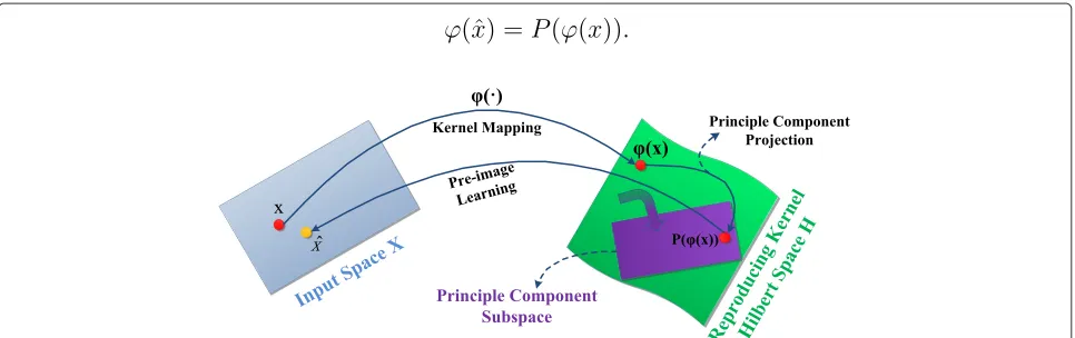
In order to obtain the input-space distance between

x and its reconstruction result, it is necessary to map

P(ϕ(x))back into the input space. The reverse mapping from feature space back to input space is called the preim-ageproblem (Figure 1). However, the preimage problem is ill-posed and the exact preimagexofP(ϕ(x))in the input

space does not exist [41]; instead, one can only find an approximationxˆin the input space such that

ϕ(xˆ)=P(ϕ(x)). (9)

In order to address the preimage learning problem, some algorithms have been proposed. Mika et al. [41] pro-posed an iterative method to determine the preimage by minimizing least square distance error. Kwok and Tsang proposed a distance constraint learning (DCL) method to find preimage by using a similar technique in multi-dimensional scaling (MDS) [42]. In a more recent work, Zheng et al. [43] proposed a weakly supervised penalty strategy for preimage learning in KPCA; however, their method needs information for both positive and negative classes. As we are only interested in one-class scenarios, the distance constraint method in [42] was selected with respect to the work described in this paper. We briefly review the method here.

For any two patternsxi andxj in the input space, the

Euclidean distanced(xi,xj) can be easily obtained.

Sim-ilarly, the feature-space distance d˜(ϕ(xi),ϕ(xj))between

theirϕ-mapped images in the feature space can also be obtained. For many commonly used kernels, such as the Gaussian kernels, there is a simple relationship between the feature-space distance and the input-space distance [44]:

˜

d_ij2=Kii+Kjj−2κ(dij2). (10)

Therefore,

κ(d2_ij)= 1

2(Kii+Kjj− ˜d 2

ij). (11)

Asκis invertible,d_ij2can be obtained ifd˜_ij2is known. A given training set hasnpatternsX= {x1,. . .,xn}. For

a patternxin the input space, the correspondingϕ(x)is projected toP(ϕ(x)), then for each training patternxiinX, P(ϕ(x))will be at a certain distanced˜(P(ϕ(x)),ϕ(xi))from

ϕ(xi)in the feature space. This feature-space distance can

be obtained by:

˜

d2(P(ϕ(x)),ϕ(x))= P(ϕ(x))2+ ϕ(xi)2

−2P(ϕ(x))ϕ(xi).

(12)

The Equation 12 can be solved by using Equations 5 and 8. Therefore, the kernel space distances in Equation 11 betweenP(ϕ(x))and eachxican be obtained now. Denote

the kernel space distance betweenP(ϕ(x))andxias:

d2=[d₁2,d2₂,. . .,d_n2] . (13)

The location ofxˆwill be obtained by requiringd2(xˆ,xi)

to be as close to the values in (13) as possible, i.e.,

d2(xˆ,xi)di2, i=1,. . .,n. (14)

To this end, in DCL, the training setX is constrained to the n nearest neighbors of x, and the least square optimization is used to obtainxˆ.

3.2 Construction of one-class KPCA ensemble for image classification

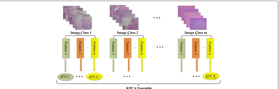
Given an image set ofmclasses, the proposed one-class KPCA ensemble is built as follows: (i) for each image cat-egory, n-type image features are extracted; (ii) a KPCA model will be trained for each individual type of the extracted features; and (iii) therefore, for each image class,

nKPCA models will be constructed. For am-class prob-lem, there will bem×nKPCA models in the ensemble. The construction of the proposed one-class KPCA ensem-ble is illustrated in Figure 2, where KPCAj_irepresents the model trained by the typejfeature from classi.

3.3 Multi-class prediction using an ensemble of one-class KPCA models

The classification confidence score is used to describe the probability of the image that belongs to each class. The confidence score can provide a quantitative measure of the predictions produced by KPCA models.

Given an unlabeled imagex with nextracted features

F = {f1,f2,. . .,fn}, let KPCAj_irepresent the KPCA model

belonging to class i and trained from the feature set fj,

wherei ∈ {1. . .m}is the class label andj ∈ {1. . .n}is the feature label. For classification, the preimages of each image feature fj ∈ F will be obtained by all the KPCA

models trained from the jth feature. The DCL method introduced in Section 3.1 is used for obtaining the preim-ages. For example, the preimages off1will be obtained by the models KPCA1_i,i = 1,. . .,m. Denote the preimages of fj asfj = {fj1,fj2,. . .,fjm}, and the squared distance Dj betweenfj andfj is used as the reconstruction error,

therefore:

Dj=[d1j,d2j,. . .,dmj ] , (15)

where dj_i = fj −fji2,i = 1,. . .,m. In the same way,

the preimages of all the features in F will be obtained, forming a distance matrix D, which has the dimensions

n×m, wherenis the number of KPCA models used for the preimage learning andmis the number of image classes. Each row ofDrepresents the reconstruction errors of a feature inFbymKPCA models from each class:

D=

⎡ ⎢ ⎢ ⎢ ⎣

D1

D2 .. .

Dn

⎤ ⎥ ⎥ ⎥ ⎦=

⎛ ⎜ ⎜ ⎜ ⎝

d1₁ d2₁ · · · d₁m d1₂ d2₂ · · · d₂m

..

. ... · · · ...

d1_n d_n2 · · · d_nm

⎞ ⎟ ⎟ ⎟

⎠. (16)

Noting that the values in each column ofDrepresents the reconstruction errors of F using the KPCA models from the same class, these values provide a measurement of how an image x is described by the KPCA models from one class. Since we try to find the KPCA mod-els from a class which give the minimum reconstruction error, this indeed is a 1-nearest neighbor search, as we wish to find the best preimage ofxinmpreimages. Such a distance measure can improve the speed of the classifi-cation. Moreover, it is also in line with the ideas in metric multi-dimensional scaling, in which smaller dissimilarities are given more weight, and in locally linear embedding, where only the local neighborhood structure needs to be preserved [42].

In order to combine the reconstruction errors from KPCA models, the reconstruction errors in D are first normalized using Equation 17:

˜

d_ij=exp(−d_ij/s), (17)

which models a Gaussian distribution from the square distance. The scale parameterscan be fitted to the distri-bution ofd_ij. Moreover, Equation 17 has the feature that the scaled value is always bounded between 0 and 1. The normalized distance matrixDis denoted byD˜.

The normalized reconstruction errors inD˜ are obtained by different one-class KPCA models, which can be com-bined to produce the confidence scores (CS) for classifying

xinto each class. LetCs = {cs1,cs2,. . .,csm}denote the

confidence scores forxwith respect to each image class. The confidence scores can be computed from the distance matrix D˜ by using an appropriate combination rule. A product rule was proposed in [45] for combining one-class classifiers:

csk(x)=

kPk(x|wT)

kPk(x|wT)+kPk(x|wO)

, (18)

wherekis the label of the target class._kPk(x|wT)is the probabilities of classifyingxinto the target class obtained from classifiers of classk, which can be calculated from the values in one column of the distance matrixD˜ as:

k

Pk(x|wT)=

j=1...n

˜

d_jk. (19)

Pk(x|wO)represents the probability ofxbelonging to the outlier class, which is obtained by multiplying all the values inD˜ except the values from the ‘target’ classk:

Pk(x|wO)= _˜

d_ji, j=1. . .n,i=1. . .mandi=k.

(20)

In [30], the authors investigated different mechanisms for combining one-class classifiers, and their results showed that the ‘product rule’ in Equation 18 outperforms other combining mechanisms for one-class classifiers. As noted in [30,45], when using the product combining rule,

Pk(x|wT) should be available and a distance should be transformed to a ‘resemblance’ by some heuristic mapping as in Equation 17.

Figure 3Illustration of KPCA model selection to produce outlier probability product.

obtained, approaching 0, which makes the classification confidence scores rather closed to each other.

Here, a variant of the product combining rule of Equation 18 is proposed to address the imbalance prob-lem. Instead of using the mapping values from all the outlier classes’ KPCA models, for those models trained by a same type of image feature, only the model that gives the biggest mapping value will be chosen to produce

kPk(x|wO). The proposed product combining rule can be described as:

csk(x)=

kPk(x|wT)

kPk(x|wT)+jP j k(x|wO)

, (21)

where j is the image feature label and j = 1. . .n.

kPk(x|wT) can be obtained using Equation 19. Each

P_kj(x|wO)injP j

k(x|wO)is the probability ofxbelongs to

the outlier classes using thejth image feature, which can be obtained by:

P_kj(x|wO)=max{ ˜d

i

j},i=1. . .mandi=k. (22)

The maximum value selection procedure in Equation 21 is illustrated by a simple example in Figure 3. In Figure 3, there is a four-class classification task (I, II, III, and IV in the figure), in which four types of features are extracted from imagex. For one type of image feature, there are four

trained KPCA models, each from a different class, giv-ing four reconstruction results for the same feature ofx

(one row in matrixD˜). If we consider classI as the ‘tar-get’ class (first column in the figure), the four values in the first column are used to produce the item_kPk(x|wT)in Equation 21. The other three column of values are deemed as the outlier probabilities produced by the KPCA mod-els from the other three classes. The proposed combining rule selects the maximum mapping value from each row to produce the outlier probability product_jP_kj(x|wO).

The selection scheme in Equation 21 ensures that the numbers of items for calculating _kPk(x|wO) and

Pk(x|wT)are the same. Moreover, the negative effect on confidence scores brought by the imbalance can also be removed. The proposed combining rule is in line with the basic idea of one-class classification, as in the one-class scenario, one only needs to know if a pattern should be assigned to the target class or to the outlier class. If one or more outlier models is able to produce a high outlier prob-ability product, the current target class should be doubted. Moreover, by combining the outliers value from different feature-derived models, the diversity of the ensemble will be improved, which is an important factor to make an ensemble learning method successful [46].

Note that since the ‘target class’ is unknown for an unlabeled image, during classification, each class will be deemed as the target class in turn to calculate the confi-dence score, i.e., each column inD˜ will be used in turn to obtain_kPk(x|wT)for each class. In such a way, for am -class -classification, each -class will be deemed as the target class, one by one, to producemconfidence scores; thus the image will be assigned to the class giving the maximum classification confidence score.

4 Experiments and results

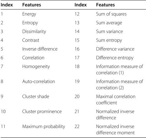
The effectiveness of the proposed method is illustrated using a biopsy breast cancer image set, a 3D OCT retinal image set, and the UCI Wisconsin breast cancer (diagnos-tic) dataset. The details of the image set and image feature extractors are given in Section 4.1. Section 4.2

Table 1 Features extracted from gray level co-occurrence matrix

Index Features Index Features

1 Energy 12 Sum of squares

2 Entropy 13 Sum average

3 Dissimilarity 14 Sum variance

4 Contrast 15 Sum entropy

5 Inverse difference 16 Difference variance

6 Correlation 17 Difference entropy

7 Homogeneity 18 Information measure of correlation (1)

8 Auto-correlation 19 Information measure of correlation (2)

9 Cluster shade 20 Maximal correlation coefficient

10 Cluster prominence 21 Normalized inverse difference

11 Maximum probability 22 Normalized inverse difference moment

duces our experimental setup and the evaluation methods used in our experiments. The effectiveness of combin-ing kernel PCAs is illustrated in Section 4.3. Finally, the proposed method was compared with some state-of-art ensemble classification methods on the UCI Wisconsin breast cancer dataset.

4.1 Image set and feature extraction

With respect to the work described in this paper, three medical image sets were used to evaluate the proposed classification method: A breast cancer benchmark biopsy images dataset from the Israel Institute of Technology [47], a 3D OCT retinal image set, and the breast cancer dataset (diagnostic) from UCI machine learning reposi-tory [48].

4.1.1 Breast cancer biopsy image set

The image set consists of 361 samples, of which 119 were classified by a pathologist as normal tissue, 102 as carcinoma in situ, and 140 as invasive ductal or lobu-lar carcinoma. The samples were generated from breast tissue biopsy slides, stained with hematoxylin and eosin. They were photographed using a Nikon Coolpix 995 attached to a Nikon Eclipse E600 (Nikon Corporation, Shinjuku, Tokyo, Japan) at magnification of×40 to pro-duce images with resolution of about 5 μper pixel. No calibration was made, and the camera was set to automatic exposure. The images were cropped to a region of interest of 760×570 pixels and compressed using the lossy JPEG compression. The resulting images were again inspected by a pathologist to ensure that their quality was sufficient for diagnosis. Figure 4 presents three sample images of healthy tissue, tumorin situ, and invasive carcinoma.

The shape feature and texture feature are critical factors for distinguishing one image from another. For the biopsy image discrimination, shapes and textures are also effec-tive. As we can see from Figure 4, the three kinds of biopsy images have visible differences in cell externality and tex-ture distribution. Thus, we use completed local binary pat-terns (CLBPs) [49] for extracting local textural features, gray level co-occurrence matrix (GLCM) [50] statistics for representing global textures, and the curvelet transform [51] for shape description. These feature descriptors have shown promising results in our previous work on biopsy image classification [52].

Different from traditional LBPs, in CLBPs a local region is represented by three coding operators to represent the central pixel, the difference signs, and the difference magnitudes [49]. According to the authors, CLBP can achieve much better rotation invariant texture classifica-tion results than convenclassifica-tional LBP-based schemes. In this paper, we use the 3D joint histogram of these three oper-ators to generate textural features of breast cancer biopsy

Figure 6Examples of OCT images.(a)Before preprocessing.(b)After preprocessing.

images, and the joint combination of the three compo-nents gives better classification than when using conven-tional LBPs and provides a smaller feature dimension. The dimension of the CLBP feature is 200.

The co-occurrence probabilities provide a second-order method for generating texture features. The basis for fea-tures used here is the gray level co-occurrence matrix [50]. With respect to the work described in this paper, a total of 22 features were extracted from gray level co-occurrence matrix, and they are listed in Table 1. Each of these statistics has a qualitative meaning with respect to the structure within the gray level co-occurrence matrix. The total dimension of the GLCM features is 220.

The fastest curvelet transform currently available is the curvelets via wrapping [51], which was therefore adopted with respect to our work. From the curvelet coefficients, some statistics can be calculated from each of these curvelet sub-bands. In this paper, the meanμ, the stan-dard deviation δ, and the entropy H are used as the simple features. If n curvelets are used for the trans-form, 3n features G =[Gμ,Gδ,H] are obtained, where Gμ =[μ1,μ2,. . .,μn], Gδ =[δ1,δ2,. . .,δn], and H =

[h1,h2,. . .,hn]. A 3n-dimensional feature vector can be

used to represent each image in the dataset. Using five levels of the curvelet transform, 82 sub-bands of curvelet coefficients are computed, therefore, a 246 dimensional curvelet feature vector is generated for each image.

4.1.2 3D OCT retinal image set

The 3D OCT retinal image set was collected at the Royal Hospital of University of Liverpool. The image set con-tains 140 volumetric OCT images, in which 68 images are

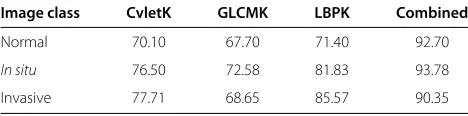
Table 2 Recognition rate (percent) for the biopsy image data from individual KPCAs and the combined model

Image class CvletK GLCMK LBPK Combined

Normal 70.10 67.70 71.40 92.70

In situ 76.50 72.58 81.83 93.78

Invasive 77.71 68.65 85.57 90.35

from normal eyes and the remainder from eyes that have age-related macular degeneration (AMD). Figure 5 shows the example images.

The OCT images are preprocessed by using the Split Bregman Isotropic Total Variation algorithm with a least squares approach [53]. The preprocessing step has two targets: (i) identification and extraction of a volume of interest (VOI) which also results in noise removal and (ii) flattening of the retina as appropriate. The example images after preprocessing can be seen in Figure 6.

As the images are three-dimensional, following the work in [53], three types image features were used for image description: local binary patterns of three orthogonal planes (LBP-TOP), local phase quantization (LPQ) and multi-scale spatial pyramid (MSSP).

4.1.3 UCI breast cancer dataset

The Wisconsin breast cancer image sets were obtained from digitized images of fine needle aspirate (FNA) of breast masses. They describe characteristics of the cell nuclei present in the image. Ten real-valued features are computed for each cell nucleus: radius, texture, perime-ter, area, smoothness, compactness, concavity, concave points, symmetry and fractal dimension. The 569 images in the dataset are categorized into two classes: benign and malignant.

4.2 Experimental setup and performance evaluation methods

MATLAB 7 was used to implement the proposed process together with the Gaussian kernelk(x,y) = exp(−x− y2/2σ2). Other types of kernels could have been used; however, since the Gaussian kernel is commonly used for the kernel PCA, the SVDD, and the Parzen density, this kernel is the only kernel used with respect to the experiments reported here.

Table 3 Recognition rate (percent) for the 3D OCT retinal image data from individual KPCAs and the combined model

Image class LPQK LBP-TOPK MSSPK Combined

Normal 86.20 88.45 85.56 92.30

AMD 86.50 86.69 85.83 91.82

• Recognition rate (RR) = number of correctly recognized images / number of testing images • ROC, receiver operating characteristic graph • AUC, area under an ROC curve

4.3 Evaluation of kernel PCA ensemble

The KPCA ensemble evaluation using the biopsy image data and the 3D OCT retinal image data is reported in this section. For the biopsy images, as introduced in Section 4.1, three types of image features were extracted, therefore for each image class, three kernel PCAs were built with respect to each type of image feature. The recognition rates of using these KPCAs individually are listed in column 2 to column 4 in Table 2, where CvletK, GLCMK, and LBPK represent KPCA models trained from curvelets, GLCM, and LBP, respectively. The results of combining all KPCA models are listed in the last col-umn of Table 2; the combining rule is introduced in Equation 21. The parameters of KPCAs were set toσ =4 andn = 40. The combined model gives the best classi-fication performance for each image class; the averaged classification accuracy for these three image classes is 92.28%.

The evaluation results on the 3D OCT retinal images are list in Table 3. Three types of image features were extracted, namely LPQ, LBP-TOP, and MSSP. Therefore, for each image class three kernel PCAs were built with respect to each type of image feature. The recognition rates of using these KPCAs individually are listed in col-umn 2 to colcol-umn 4 in Table 3, where LPQK, LBPK, and MSSPK represent the KPCA models trained from LPQ, LBP-TOP, and MSSP, respectively. The results of com-bining all KPCA models are listed in the last column of Table 3. The parameters of KPCAs were set toσ =4 and

n=40. The combined model gives the best classification

Table 4 Recognition rate (percent) for biopsy image data from different one-class classifier ensembles

Image class PCA MoG KMeans SVDD Parzen KPCA

Normal 85.17 82.12 80.12 85.56 84.54 92.70

In situ 87.33 84.67 83.46 87.22 81.26 93.78

Invasive 82.56 81.88 79.65 84.67 83.23 90.35

The kernel widths for KPCA and SVDD were set toσ= 4. The number of principal components for KPCA and PCA were set ton= 40.

Table 5 Recognition rate (percent) for 3D OCT retinal image data from different one-class classifier ensembles

Image class PCA MoG KMeans SVDD Parzen KPCA

Normal 82.06 84.56 76.96 88.77 82.04 92.30

AMD 81.22 85.67 78.84 86.45 80.73 91.82

The kernel widths for KPCA and SVDD were set toσ= 4. The number of principal components for KPCA and PCA were set ton= 40.

performance for each image class; the averaged classifica-tion accuracy for these two image classes is 92.06%.

From Tables 2 and 3, one can see that using the pro-posed product combining rule, the classification accura-cies of all the image classes have been improved. This illustrates that by combining one-class classifiers trained from different features can improve the classification per-formance, which is in accordance with the observation in [30]. For comparison, the other one-class classifiers are also used as the base classifier of the ensemble, using the same combining rule, the classification results on the biopsy image set and the 3D OCT retinal image set are listed in Tables 4 and 5, respectively.

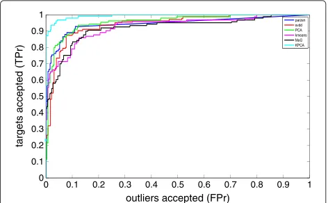
With respect to the comparison of the operation of a variety of one-class classifiers, six one-class classifiers were used as the base classifier for the ensemble: they are Parzen, SVDD, PCA, Kmeans, MoG, and KPCA. The receiver operating characteristic (ROC) curves obtained using different one-class classifiers on the biopsy image data are shown in Figure 7. Thexaxis of the ROC curves is false positive rate (FPr) and the y axis is the true positive rate (TPr). The FPr and TPr are obtained by Equations 23 and 24, respectively. A threshold on the difference between the biggest confidence score and the second biggest confidence score was used to obtain the trade-off between TPr and FPr. Initially, the threshold was set to 0.05, then the threshold was increased by a step of 0.01 until 0.60, on each threshold value, and the TPr

1

0.9

0.8

0.7

0.6

0.5

0.4

0.3

0.2

0.1

0

1 0.9 0.8 0.7 0.6 0.5 0.4 0.3 0.2 0.1 0

outliers accepted (FPr)

targets accepted (TPr)

Table 6 AUC of different one-class classifiers used as the base classifier for the ensemble on the biopsy image data

Parzen SVDD PCA Kmeans MoG KPCA

AUC 84.30 83.61 84.19 84.28 83.67 93.53

and FPr were accounted. The areas under the ROC curves (AUC), for the compared classifiers, are listed in Table 6; the KPCA ensemble gives the best result.

TPr= True positive

True positive + False negative (23)

FPr= False positive

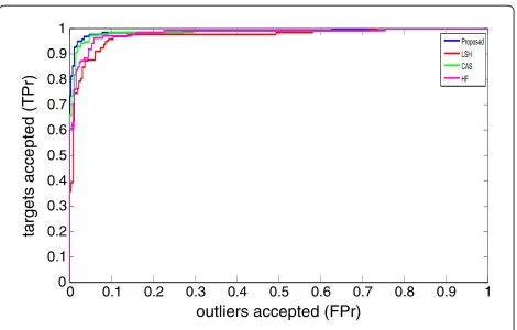
False positive + True negative (24) The proposed method was also compared with some state-of-art methods on the biopsy image set. The meth-ods compared with are as follows: (i) the level set his-togram (LSH) method proposed in [54]; (ii) a cascade classification system (CAS) in [55], which first classi-fies the images into ‘cancer’ and ‘non-cancer’ categories, then further classification is implemented within the ‘can-cer’ category to discriminate different cancer types; (iii) a hybrid feature (HF) proposed in [56], which used higher-order spectra (HOS), local binary pattern (LBP), and laws texture energy (LTE) for histopathological image clas-sification, in which the Takagi-Sugeno fuzzy model is selected as the classifier.

In our experiment, based on the description in [54], for LSH, the images were first converted to grayscale images that have the intensity range between 0 and 255, then 25 thresholds with the steps of 10 were used to convert the images into binary images (0 and 1). For each binary image, the level set segmentation was used to generate a 42-bin histogram for the connected components in the image. Thus, each image finally generated a feature vector with the size of 42×25 = 1, 050. SVM with RBF ker-nel was used for classification with the parameterσ that defines the spread of the radial function set to 4.0, and the parameterC that defines the trade-off between the clas-sifier accuracy and the margin was set to 3.0. For CAS, we used the same classifier, decision tree C5.0, and the same image features as stated in [55]. The feature vector for each image is a combination of first-order statistics, co-occurrence matrix, and steerable filters.

Table 7 Performance comparison of some state-of-art methods and the proposed method on the biopsy image set

Classification accuracy Error rate AUC

LSH 87.38 13.62 88.97

CAS 91.94 7.88 93.12

HF 90.27 9.73 91.56

Proposed 92.28 7.72 93.85

1

0.9

0.8

0.7

0.6

0.5

0.4

0.3

0.2

0.1

0

1 0.9 0.8 0.7 0.6 0.5 0.4 0.3 0.2 0.1 0

outliers accepted (FPr)

targets accepted (TPr)

Figure 8Receiver operating characteristics curves of the compared methods on the biopsy image data.

Table 7 lists the performance of the compared methods on the biopsy image set, where one can be noted that the proposed method achieved the better performance than other methods. The CAS method obtained an accuracy of 91.94%, which is superior than the accuracy of LSH and HF. The LSH method obtained only 87.38% accu-racy on the biopsy image set. LSH only used the level set histograms for image description, while other com-pared methods all used composite image features, which demonstrates that using a combination of different image features can improve classification performance. Figure 8 presents the ROC curves of the compared methods; the AUC of the ROC curves are listed in Table 7.

For the 3D OCT retinal images, a method in [53] was used to compare with the proposed method. The method in [53] used the same image data, and the same image features introduced in Section 4.1.2 were composed together as the image feature, in which Bayes classifier was used for classification. A classification accuracy of 91.50% was reported by the authors, while our proposed system achieved 92.06%.

The proposed method was also compared with some state-of-art methods on the UCI breast cancer dataset. The methods compared are the following: (i) the multi-layer perceptron ensemble (MLPE) method proposed in [57]; (ii) a boosted neural network (BoostNN) classifier in [58]; (iii) a decision tree (DT) and support vector machine sequential minimal optimization (SVM-SMO) based ensemble classifier proposed by Luo and Cheng [59]. The results are listed in Table 8.

Table 8 Comparison of classification accuracy on the UCI breast cancer image set

MLPE BoostNN DT-SVM-SMO Proposed

5 Conclusions

In this paper, a classification scheme based on a one-class KPCA model ensemble has been proposed for the classification of medical images. The ensemble consists of one-class KPCA models trained using different image features from each image class, and a proposed prod-uct combining rule was used for combining the kernel PCA models to produce classification confidence scores for assigning an image to each class. The effectiveness of the proposed classification scheme was verified using a breast cancer biopsy image dataset and a 3D OCT retinal image set. The proposed classification scheme obtained high classification accuracy on the tested image sets.

Although the proposed system has shown promising results with respect to the biopsy image classification task, there are still some aspects that need to be further inves-tigated. The benchmark images used in this work were cropped from the original biopsy scans and only cover the important areas of the scans. However, it is often dif-ficult to find regions of interest (ROIs) that contain the most important tissues in biopsy scans; therefore, more effort needs to be put into detecting ROIs from biopsy images. The parameters of the kernel PCA models, such as the number of principle components and the width of the Gaussian kernel, were fixed during the experiments. In the future research, some optimization methods or adaptive algorithms should be considered for searching the optimal parameters of KPCA models.

Competing interests

The authors declare that they have no competing interests.

Acknowledgements

The project is funded by Natural Science Foundation China grants 61262070 and EIN2011A001 and China Yunnan Provincial Natural Science Foundation grant 2010CD047.

Author details

1_{Key Laboratory of Education Informalization for Nationalities, Yunnan Normal} University, Ministry of Education, Kunming 650500, China.2_{Department of} Computer Science, University of Liverpool, Liverpool L693BX, UK.3Department of Computer Science and Software Engineering, Xi’an Jiaotong-Liverpool University, Suzhou 215123, China.4Department of Electrical and Electronic Engineering, Xi’an Jiaotong-Liverpool University, Suzhou 215123, China.

Received: 22 June 2013 Accepted: 15 January 2014 Published: 7 February 2014

References

1. LE Boucheron, Object- and spatial-level quantitative analysis of multispectral histopathology images for detection and characterization of cancer. Thesis, University of California Santa Barbara, 2008

2. C Loukas, A survey on histological image analysis-based assessment of three major biological factors influencing radiotherapy: proliferation, hypoxia and vasculature. Comput. Methods Programs Biomed.74(3), 183–199 (2004)

3. N Orlov, L Shamir, T Macura, J Johnston, DM Eckley, IG Goldberg, WND-CHARM: multi-purpose image classification using compound image transforms. Pattern Recognit. Lett.29(11), 1684–1693 (2008) 4. L Kuncheva, J Rodriguez, C Plumpton, D Linden, S Johnston, Random

subspace ensembles for FMRI classification. IEEE Trans. Med. Imaging. 29(2), 531–542 (2010)

5. D Tax, One-class classification. Thesis, Delft University of Technology, 2001 6. L Rokach, Ensemble-based classifiers. Artif. Intell. Rev.33, 1–39 (2010) 7. K-S Goh, EY Chang, B Li, Using one-class and two-class SVMs for multiclass

image annotation. IEEE Trans. Knowl. Data Eng.17(10), 1333–1346 (2005) 8. C Bergamini, L Oliveira, A Koerich, R Sabourin, Combining different

biometric traits with one-class classification. Signal Process.89, 2117–2127 (2009)

9. MS Haghighi, A Vahedian, HS Yazdi, Creating and measuring diversity in multiple classifier systems using support vector data description. Appl. Soft Comput.11, 4931–4942 (2011)

10. R Bryll, R Guitierrez-Osuna, F Quek, Attribute bagging: improving accuracy of classifier ensembles by using random feature subsets. Pattern Recognit.36, 1291–1302 (2003)

11. L Kuncheva, LC Jain, Designing classifier fusion systems by genetic algorithms. IEEE Trans. Evol. Comput.4(4), 327–336 (2000) 12. L Zhang, L Zhang, On combining multiple features for hyperspectral

remote sensing image classification. IEEE Trans. Geoscience Remote Sensing.50(3), 879–893 (2012)

13. J Yu, F Lin, H-S Seah, C Li, Z Lin, Image classification by multimodal subspace learning. Pattern Recognit. Lett.33, 1196–1204 (2012) 14. M Moya, M Koch, L Hostetler, One-class classifier networks for target

recognition applications, inProceedings of World Congress on Neural

Networks, (Portland, July 1993), pp. 797–801

15. SS Khan, MG Madden, A survey of recent trends in one class classification,

inArtificial Intelligence and Cognitive Science,Lecture Notes in Computer

Science, vol. 6206, eds. by L Coyle, J Freyne (Springer, Berlin, Heidelberg, 2010), pp. 188–197

16. M Markou, S Singh, Novelty detection: a review-part 1: statistical approaches. Signal Process.83, 2481–2497 (2003)

17. M Markou, S Singh, Novelty detection: a review-part 2: neural network based approaches. Signal Processing.83, 2499–2521 (2003)

18. DM Tax, RP Duin, Support vector domain description. Pattern Recognit. Lett.20, 1191–1199 (1999)

19. DM Tax, RP Duin, Support vector data description. Mach. Learn.54, 45–66 (2004)

20. B Schölkopf, J Platt, J Shawe-Taylor, A Smola, RC Williamson, Estimating the support of a high dimensional distribution. Neural Comput.13(7), 1443–1472 (2001)

21. LM Manevitz, M Yousef, One-class SVMs for document classification. J. Mach. Learn. Res.2, 139–154 (2001)

22. Lewis DD, Test collections - Reuters-21578. http://www.daviddlewis.com/ resources/testcollections/reuters21578. Accessed 22 June 2013 23. V Roth, Kernel fisher discriminants for outlier detection. Neural Comput.

18, 942–960 (2006)

24. D Ridder, D Tax, D Duin, An experimental comparison of one-class classification methods, inProceedings of the 4th Annual Conference of the

Advanced School for Computing and Imaging(Delft, Holland, 1998),

pp. 213–218

25. Q Wang, L Lopes, D Tax, Visual object recognition through one-class learning, inInternational Conference on Image Analysis and Recognition,

Porto, Portugal (Springer, Berlin, 2004), pp. 463–470

26. K Beyer, J Goldstein, R Ramakrishnan, U Shaft, When is ‘nearest neighbor’ meaningful? Lect. Notes Comput. Sci.540, 217–235 (1999)

27. JIT,Principal Component Analysis. (Springer, New York, 1986)

28. H Zhang, W Huang, Z Huang, B Zhang, A kernel autoassociator approach to patter classification. IEEE Trans. Syst., Man Cybernetics-Part B: Cybern. 35(3), 593–606 (2005)

29. H Hoffmann, Kernel PCA for novelty detection. Pattern Recognit.40, 863–874 (2007)

30. DM Tax, RP Duin, Combining one-class classifiers, inProceedings of

Multiple Classifier Systems(Springer, Berlin, 2001), pp. 299–308

31. AD Shieh, DF Kamm, Ensembles of one class support vector machines, in

Proceedings of the Multiple Classifier Systems(Springer, Berlin, 2009),

pp. 181–190

32. AK Jain, RPW Duin, J Mao, Statistical pattern recognition: a review. IEEE Trans. Pattern Anal. Mach. Intell.22(1), 4–37 (2000)

33. R Perdisci, G Gu, Using an ensemble of one-class SVM classifiers to harden payload-based anomaly detection systems, inProceedings of the IEEE

International Conference on Data Mining (ICDM 2006)(IEEE Computer

Society, Piscataway, 2006), pp. 488–498

34. B Krawczyk, Diversity in ensembles for one-class classification, inAdvances

information systems, vol. 185, eds. by M Pechenizkiy, M Wojciechowski (Springer, Berlin, Heidelberg, 2013), pp. 119–129

35. P Yang, YH Yang, BB Zhou, AY Zomaya, A review of ensemble methods in bioinformatics. Curr. Bioinformatics.5(4), 296–308 (2010)

36. P Li, KL Chan, SM Krishnan, Learning a multi-size patch-based hybrid kernel machine ensemble for abnormal region detection in colonoscopic images, inProceedings of the International Conference on Computer Vision

and Pattern Recognition (CVPR 2005)(IEEE Computer Society, Piscataway,

2005), pp. 670–675

37. P Li, KL Chan, S Fu, SM Krishnan, An abnormal ecg beat detector approach for long-term monitoring of heart patients based on hybrid kernel machine ensemble, inProceedings of the International Workshop on

Multiple Classifier Systems (MCS 2005)(Springer, Heidelberg, 2005),

pp. 346–355

38. O Okun, H Priisalu, Dataset complexity in gene expression based cancer classification using ensembles of k-nearest neighbors. Artif. Intell. Med. 45, 151–162 (2009)

39. B Schölkopf, The kernel trick for distances. Technical report MSR-TR-2000-51, Microsoft Research, Microsoft Corporation, One Microsoft Way, Redmond, WA 98052 (2000)

40. M Kallas, P Honeine, C Richard, C Francis, H Amoud, Non-negativity constraints on the pre-image for pattern recognition with kernel machines. Pattern Recognit.46, 3066–3080 (2013)

41. S Mika, B Schölkopf, A Smola, K-R Müller, M Scholz, G Rätsch, Kernel PCA and de-noising in feature spaces, inProceedings of the 1998 Conference on

Advances in Neural Information Processing Systems II(MIT Press, Cambridge,

1998), pp. 536–542

42. JT-Y Kwok, IW-H Tsang, The pre-image problem in kernel methods. IEEE Trans. Neural Netw.15(6), 1517–1525 (2004)

43. W-S Zheng, J Lai, PC Yuen, Penalized preimage learning in kernel principle component analysis. IEEE Trans. Neural Netw.21(4), 551–570 (2010) 44. C Williams, On a connection between kernel PCA and metric

multidimensional scaling, inAdvances in Neural Information Processing

Systems 13, NIPS 2001(MIT Press, Cambridge, 2001), pp. 675–681

45. J Kitten, M Hate, RP Duin, J Matas, On combining classifiers. IEEE Trans. Pattern Anal. Mach. Intell.20(3), 226–239 (1998)

46. LI Kuncheva,Combining Pattern Classifiers: Methods and Algorithms. (Wiley, New York, 2004)

47. Breast cancer data. ftp://ftp.cs.technion.ac.il/pub/projects/medic-image. Accessed 22 June 2013

48. UCI, Machine learning repository. http://archive.ics.uci.edu/ml/datasets/. Accessed 22 June 2013

49. Z Guo, L Zhang, D Zhang, A completed modeling of local binary pattern operator for texture classification. IEEE Trans. Image Process.19(6), 1657–1663 (2010)

50. R Haralick, K Shanmugam, I Dinstein, Textural features for image classification. IEEE Trans. Syst., Man Cybern.3(6), 610–621 (1973) 51. E Candes, L Demanet, D Donoho, L Ying, Fast discrete curvelet transforms.

Multiscale Model. Simul.5, 861–899 (2006)

52. Y Zhang, B Zhang, F Coenen, W Lu, Breast cancer diagnosis from biopsy images with highly reliable random subspace classifier ensembles. Mach. Vis. Appl, 1–17 (2012). doi:10.1007/s00138-012-0459-8

53. A Albarrak, F Coenen, Y Zheng, Age-related macular degeneration identification in volumetric optical coherence tomography using decomposition and local feature extraction, inProceedings of 2013 International Conference on Medical Image, Understanding and Analysis

(University of Birmingham, 17–19 July 2013), pp. 59–64

54. A Brook, R El-Yaniv, E Isler, R Kimmel, R Meir, D Peleg, Breast cancer diagnosis from biopsy images using generic features and SVMs. Technical report CS-2008-07, Technion-Israel Institute of Technology, Technion City, Haifa 32000, Isreal (2006)

55. S Doyle, MD Feldman, N Shih, J Tomaszewki, A Madabhushi, Cascaded discrimination of normal, abnormal, and confounder classes in histopathology: Gleason grading of prostate cancer. BMC Bioinformatics. 13(282), 1–15 (2012)

56. MMR Krishnan, V Venkatraghavan, UR Acharya, M Pal, RR Paul, LC Min, AK Ray, J Chatterjee, C Chakraborty, Automated oral cancer identification using histopathological images: a hybrid feature extraction paradigm. BMC Bioinformatics.13(282), 1–15 (2012)

57. R Valdovinos, J Sanchez, Performance analysis of classifier ensembles: neural networks versus nearest neighbor rule. Pattern Recognit Image

Anal. (Lecture Notes in Computer Science).4477, 105–112 (2007)

58. S Gou, H Yang, L Jiao, X Zhuang, Algorithm of partition based network boosting for imbalanced data classification, inProceedings of the 2010

International Joint Conference on Neural Networks, IJCNN’10(IEEE,

Piscataway, 2010), pp. 1–6

59. S Luo, B Cheng, Diagnosing breast masses in digital mammography using feature selection and ensemble methods. J. Med. Syst.36(2), 569–577 (2012)

doi:10.1186/1687-6180-2014-17

Cite this article as:Zhanget al.:One-class kernel subspace ensemble for medical image classification.EURASIP Journal on Advances in Signal Processing 20142014:17.

Submit your manuscript to a

journal and benefi t from:

7 Convenient online submission 7 Rigorous peer review

7 Immediate publication on acceptance 7 Open access: articles freely available online 7 High visibility within the fi eld

7 Retaining the copyright to your article