CEMSYS modelled wind erosion

CEMSYS MODELLED WIND

EROSION

Prepared by:

John Leys, Harry Butler, Xihua Yang, Stephan Heidenreich

Acknowledgments

This project was supported by the Department of Environment, Climate Change and Water NSW

through funding from the Australian Government’s Caring for Our Country. The authors thank

Dr Michele Barson (Department of Agriculture, Fisheries and Forestry, Sustainable Resource

Management) for her advice and encouragement.

Published by:

Department of Environment, Climate Change and Water NSW on behalf of the

Department of Environment, Water, Heritage and the Arts

59-61 Goulburn Street

PO Box A290

Sydney South 1232

Phone: (02) 9995 5000 (switchboard)

Phone: 131 555 (environment information and publications requests)

Phone: 1300 361 967 (national parks, climate change and energy efficiency information and

publications requests)

Fax: (02) 9995 5999

TTY: (02) 9211 4723

Email: info@environment.nsw.gov.au

Website: www.environment.nsw.gov.au

ISBN 978 1 74232 635 1

DECCW 2010/321

June 2010

Copyright © 2010 Commonwealth of Australia.

Contents

Page

Executive Summary ... v

1.

Introduction ... 1

1.1

Project Team... 1

1.2

Project Objectives ... 1

2.

Study Methods ... 2

2.1 Model simulation ... 2

2.1.1. The atmospheric model... 3

2.1.2. The land surface model... 5

2.1.3. The wind erosion model ... 5

2.2 Developing the NRM Regional Map For Wind Erosion Reporting... 10

2.3 Calculation of Statistics ... 12

3.

Results and Discussion ... 14

3.1 Monthly Data ... 14

3.2 Annual Dust-year Data ... 20

4.

CEMSYS Implementation Plan ... 29

4.1 Background ... 29

4.2 Proposed Improvements ... 31

4.3 Proposed Products... 32

4.4 Costing ... 33

5.

Conclusions... 34

6.

References... 36

Appendix 1: NRM regions and sub regions... 38

Sorted by region number... 38

Sorted by region name ... 39

Appendix 2. Monthly statistics for each NRM region, state and the continent ... 41

Figures

Page

Figure 1. The framework of the CEMSYS model ... 2

Figure 2. The nesting procedure of the atmospheric model:... 4

Figure 3. The soil (a) and vegetation (b) map classes used in CMESYS for Australia. ... 9

Figure 4. NRM regions and subregions... 11

Figure 5. Modelled monthly wind erosion maps for the period July 2006 to June 2007... 15

Figure 6. Modelled monthly wind erosion maps for the period July 2007 to June 2008... 16

Figure 7. Comparison of 10-km and 50-km CEMSYS products for the percentage of the CMA

area in the high and very-high erosion classes ... 18

Figure 8. Calculated monthly average wind fields (m/s) for February 2008 at 50-km resolution

(a) and 10-km resolution (b). ... 18

Figure 9. Contour maps illustrating the spatial variability in wind speed (m/s) for February

2008 at 50-km (a) and 10-km (b) resolutions ... 19

Figure 10. Wind erosion classes for national annual average dust storm years for 2006–07

and 2007–08 at 50-km resolution... 24

Figure 11. Rainfall decile maps for the 2006–07 and 2007–08 dust-years ... 25

Figure 12. Location of 110 BoM stations used to map DSI (After McTainish

et al.

2010) .... 27

Figure 13. CEMSYS (above) and DSI (below) maps for 2007–08 ... 28

Figure 14. CEMSYS outputs for NSW for 2007–08 at 50 and 10-km resolution... 30

Figure 15. CEMSYS 2007–08 map of Australia at 50-km resolution, with 10-km resolution

within NSW... 32

Tables

Page

Table 1. USDA soil classifications... 6

Table 2. Summary of soil mapping units and soil properties... 7

Table 3. Summary of vegetation mapping units ... 8

Table 4 Estimated soil loss rates in t/km

under three erodibility scenarios in the Channel

Country of western Queensland... 19

Executive Summary

The Leys report on wind and water erosion (Leys

et al.

2009b) recommended that wind

erosion modelling be undertaken to assist in reporting the extent and severity of wind erosion

across Australia. The modelling could then be used by the Australian Government, states

and Natural Resource Management (NRM) bodies for resource condition reporting. The

same products could be used to assist in identifying areas for Caring for our Country (C4oC)

investments.

Modelled monthly and annual wind erosion maps of Australia at 50-km resolution for the

period July 2006 to June 2008 were compiled using the Computational Environmental

Management System model (CEMSYS). CEMSYS comprises an atmospheric model, a land

surface model, a wind erosion model, a transport and deposition model and a land surface

database. It uses analysis data from the National Centre for Environmental Prediction, USA

(NCEP) to calculate the atmospheric properties like wind fields, rainfall, radiation and clouds.

Geographic Information Systems (GIS) are used to describe soils and vegetation data and

monthly satellite data is used to calculate ground cover levels. In this study, the severity of

wind erosion is described by the horizontal soil flux (TQ mg/m/s) output from CEMSYS. TQ is

representative of the average amount of soil that is moved by wind within the pixel each

month.

To aid with reporting, a modified map of NRM regions and subregions was developed by an

expert panel to report wind erosion status. The severity of erosion, expressed as five erosion

classes (very low to very high), was then calculated for each subregion, region, state and the

continent for 24 months.

In the 2007–08 dust-year 11% of Australia was in the high and very high erosion classes.

This compares to 9% of Australia in the 2006–07 dust-year; however, this 2% yearly

difference is not statistically significant. NRM regions with the largest areas of erosion (high

and very high classes) tend to be focused in arid and semi-arid rangelands of south-western

Queensland, western NSW, north-central and north-eastern South Australia and western

Western Australia. The semi-arid agricultural lands of eastern West Australia also had areas

of high and very high class erosion. Notably, the non-agricultural lands of western South

Australia, northern Northern Territory and eastern Western Australia all have low erosion

levels.

The NRM regions, by state, with the highest amounts of soil moved (TQ) were:



Desert Channels, South West, Border Rivers Maranoa–Balonne, and Condamine in

Queensland



Western, Border Rivers–Gwydir, Namoi, Lachlan, Murrumbidgee, Murray and Lower

Murray–Darling regions in NSW



the Arid Lands and Northern and Yorke regions of South Australia



the Pastoral and Non-Pastoral regions of the Northern Territory, and

The CEMSYS map outputs produced in this study offer a greater temporal (monthly) and

spatial resolution (50 km) and better statistical descriptions than the previous measure of

wind erosion, the Dust Storm Index (DSI). DSI maps are derived from Bureau of Meteorology

observer data from 110 sites across Australia at annual time steps. Maps are then created by

interpolating between the 110 sites. Despite the temporal and spatial limitations of the DSI, it

still remains a very valuable cross validation for CEMSYS and it has the major advantage of

a longer time series (1960 to the present).

With the exception of the annual DSI data, there is a lack of wind erosion data to test the

model outputs against at the 50 and 10-km scales. Roadside survey data from NSW is

one-hectare scale data and was used to determine the five erosion severity classes and therefore

could not be used to test the model. Future testing is planned after the compilation of

DustWatch data and roadside survey data from other states (South Australia and Western

Australia).

Model outputs appear to be most reliable in the south-eastern Australian rangelands.

Outputs for the savannas and grasslands of northern Australia seem less reliable due to the

lack of accuracy of the satellite ground cover product’s ability to detect dead or senescing

vegetation. This error in cover estimates results in an over-prediction of erosion in northern

Australia. Under-prediction of erosion in the winter cropping areas of southern Australia is

noted and possibly relates to the simplification of soil types used in the model. The model’s

performance will be improved by using better ground cover and soils data and projects are

underway to address these data issues.

The issue of scaling needs to be appreciated and this project shows the problems of

comparing data measured at different scales (10 and 50 km) and the loss of precision at 50

km. Larger pixels involve greater averaging of underlying information and as such the

likelihood of reporting high and low values is reduced. Therefore, the chance of locating

areas with high levels of wind erosion is reduced. In this study, the scalded river margins

along the Edward and Wakool Rivers in the western end of the Murray catchment

management area were classified ‘High’ and ‘Very High’ at 10-km resolution and ‘Low’ and

‘Moderate’ with the 50-km resolution. With the 50-km data, this priority area would not have

been identified.

1. Introduction

The Leys report on wind and water erosion (Leys

et al.

2009b) recommended that wind

erosion modelling be undertaken to assist in reporting the extent and severity of wind erosion

across Australia. The modelling could then be used by the Australian government, states and

Natural Resource Management (NRM) bodies for resource condition reporting. The same

products would also assist in identifying areas for Caring for our Country (C4oC)

investments.

This report was commissioned by the Australian Government as represented by the

Department of the Environment, Water, Heritage and the Arts with funding from the Caring

for our Country initiative.

This project aims to make available monthly maps of wind erosion and statistics on wind

erosion rates. The maps and statistics are based on modelled data produced at 50 km

resolution for the Australian continent, state and NRM regions for period July 2006 to June

2008.

1.1 PROJECT

TEAM

A collaborative effort between the Department of Environment, Climate Change and Water

NSW (DECCW) and the University of Southern Queensland (USQ) was required to complete

this project. Protect team members were Dr John Leys (DECCW), Dr Harry Butler (USQ),

Dr Xihua Yang (DECCW) and Mr Stephan Heidenreich (DECCW).

1.2 PROJECT

OBJECTIVES

The objectives of this project were:



to provide modelled monthly maps and statistics on the intensity and extent of wind

erosion at Australian continental, state and NRM scales for July 2006 to June 2007, and



to develop a four-year implementation plan (2009–12) outlining the provision of higher

2. Study

Methods

Several steps were required to complete the project’s objectives. These are described in

detail in this section and are summarised as:



Run the CEMSYS model and create the American Standard Code for Information

Interchange (ASCII) output files.



Produce an NRM region map of the country suitable for reporting the statistics on wind

erosion.



Convert the ASCII files to ArcGIS grid files and write ArcGIS script files to calculate the

monthly and dust-year statistics for each NRM region, state and national area.



Produce maps of wind erosion for each month and dust-year.

2.1 MODEL SIMULATION

The Computational Environmental Management System model (CEMSYS) (Shao

et al.

2007) was used to model wind erosion for the period 1 July 2006 to 30 June 2008. The

following summary of the model is from Leys

et al.

(2009b p.18) and Butler

et al.

(2008).

‘CEMSYS has been under development since the early 1990s (Shao

et al.

1996; Shao and

Leslie 1997; Shao 2003; Shao

et al.

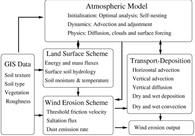
2007). As Figure 1 shows, CEMSYS comprises an

atmospheric model, a land surface model, a wind erosion model, a transport and deposition

model, and a land surface database. The atmospheric model has treatments for atmospheric

dynamic and physical processes, including radiation, clouds, convection, turbulent diffusion,

and the atmospheric boundary layer (Leslie and Wightwick 1995).

Figure 1. The framework of the CEMSYS model

The wind erosion model obtains friction velocity and soil moisture from land surface models,

and other spatial parameters from the GIS database, and predicts sand and dust fluxes. To

predict dust motion, the transport and deposition model obtains wind fields, turbulent

diffusivities and precipitation from the atmospheric model, and dust flux and particle size

information from the wind erosion model. The atmospheric model is run first, followed by the

land surface model and the wind erosion model. Finally, calculations of dust transport and

deposition are done.’

The sub-models are outlined in more detail in the following sections.

2.1.1. The atmospheric model

The simulation is completed in two stages. In Stage 1 CEMSYS is run over the Australian

region at 50 km horizontal resolution and 25 levels in vertical. The atmospheric boundary

layer is resolved using 10 levels from 850 hPa to the surface, with the lowest level at a few

metres. Initial and boundary conditions for this atmospheric model are obtained using

analysis data from the National Centre for Environmental Prediction, USA (NCEP).

Stage 2 involves running CEMSYS at a finer 10 km horizontal resolution. In this stage, the

atmospheric model is self-nested; that is, the atmospheric model derives its initial and

a)

Average Temperature (

C) and Average Wind Speed (m/s) on 10 February 2008.

b)

Average Temperature (

C) and Average Wind Speed (m/s) on 10 February 2008.

Figure 2. The nesting procedure of the atmospheric model:

2.1.2. The land surface model

The wind erosion threshold friction velocity (u

) is strongly related to soil moisture. The

evolution of soil moisture depends on surface hydrological processes and the interactions

between the atmosphere and the land surface, because such interactions determine the

evaporation, and to a certain degree, precipitation. In this study, soil moisture is simulated

within the land surface model using atmospheric and land surface data.

The land surface model can incorporate as many soil layers as required to provide a better

vertical resolution of soil moisture and better treatment of heterogeneity (in the vertical) of

soil hydraulic properties. This flexibility in choosing the number of soil layers also facilitates a

better simulation of soil moisture close to the surface, which is important in estimating

threshold friction velocity.

In the model, the land surface is divided into areas of bare soil and vegetation. The energy

transfer processes over bare soil surfaces and canopies are described using aerodynamic

resistance laws (Irannejad and Shao 1998).

2.1.3. The wind erosion model

The friction velocity (u

) is calculated from the land surface data and the atmospheric data.

The surface resistance is represented by the threshold friction velocity (u

) and is dependent

on the particle size of the soil surface, atmospheric conditions and surface conditions such

as soil moisture, vegetation cover and soil type as described by (Shao and Lu 2000).

Under natural conditions, silt and clay particles may occur as individual grains, as

aggregates, or as coatings upon sand grains. During a minor wind erosion event, soil

aggregates behave in a similar fashion to sand particles. However, as wind erosion

intensifies, these aggregates can break or abrade, releasing dust into the air. Therefore,

CEMSYS uses two types of particle size-distributions. The first particle size-distribution

involves as little as possible disturbance to the soil sample (minimally dispersed). The

second particle size-distribution reduces the soil to its fundamental particle sizes (fully

dispersed). The dispersed particle distribution approximates a sediment particle

size-distribution during strong wind erosion events. Both the minimally dispersed and fully

dispersed particle size-distributions are used in the computation of the streamwise saltation

flux of sand particles and the emission rate of dust particles. In this study, only five of the

12 soil classifications used were available for both minimally and fully dispersed distributions.

This simplification of the soils data is recognised and more soils are being analysed as part

of a sister project to overcome this limitation (McTainsh

et al.

2010).

The soil and vegetation types are derived from the geographic data from the

Atlas of

Australian Resources

(AAR) Volumes 3 (NATMAP 1980) and 6 (AUSLIG 1990). The spatial

resolution of the data is 5x5 km.

Australian soils are classified into 28 soil-map classes within AAR, with 21% being shallow

permeable sandy soils, 17% deep massive earths, 11.2% cracking clay soils with low

permeability when wet, 11% shallow loam soils, 8.4% sandy soils, 5.4% calcareous earths

and the rest of the soil types occupy 26%. Based on the qualitative description of the soil

properties and associated landforms of each soil, the 28 soil-map classes are regrouped into

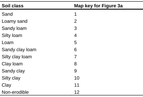
the 12 United States’ Department of Agriculture (USDA) soil-texture classes (Table 1)

corresponding soil-texture classes. For soil moisture simulation, each soil class is also

assigned a set of hydrological parameters.

Table 1. USDA soil classifications

Soil class Map key for Figure 3a

Sand 1

Loamy sand 2

Sandy loam 3

Silty loam 4

Loam 5

Sandy clay loam 6

Silty clay loam 7

Clay loam 8

Sandy clay 9

Silty clay 10

Clay 11

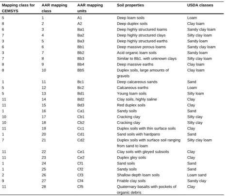
Table 2. Summary of soil mapping units and soil properties

Note that the descriptions of the soil properties are extracted from more detailed descriptions given in

Atlas of Australian Resources Volume 3 (NATMAP 1980). The corresponding CEMSYS classes and

USDA soil texture classes are also listed.

Mapping class for CEMSYS

AAR mapping class

AAR mapping units

Soil properties USDA classes

5 1 A1 Deep loam soils Loam

8 2 A2 Deep duplex soils Clay loam

6 3 Ba1 Deep highly structured loams Sandy clay loam

7 4 Ba2 Deep highly structured clays Silty clay loam

3 5 Ba3 Deep highly structured earths Sandy loam

6 6 Bb1 Deep massive porous loams Sandy clay loam

3 7 Bb2 Acid organic loam soils Sandy loam

7 8 Bb3 Similar to Bb1, with unknown clays Silty clay loam

8 9 Bb4 Deep massive earths Clay loam

8 10 Bb5 Duplex soils, large amounts of

gravels

Clay loam

1 11 Bc1 Deep calcareous sands Sand

5 12 Bc2 Calcareous earths Loam

5 13 Bd1 Young loam soils Silty loam

11 14 Bd2 Clay soils, highly saline Clay

11 15 Bd3 Red duplex soils Clay

1 16 Ca1 Sandy soils Sand

10 17 Cb1 Cracking clay Silty clay

10 18 Cb2 Cracking clay Silty clay

11 19 Cc1 Duplex soils with thin surface soils Clay

1 20 Cd1 Sand soils with hardpans Sand

7 21 Cd2 Duplex soils with surface soil ranging

from sand to loam

Silty clay loam

11 22 Ce1 Clay soils with gleyed subsoils Clay

11 23 Ce2 Duplex gley soils Clay

1 24 Cf1 Sand soils Sand

1 25 Cf2 Sandy soils Sand

2 26 Cf3 Shallow depth loam soils Loam sand

9 27 Cf4 Friable clay soils Sandy clay

11 28 Cf5 Quaternary basalts with pockets of

organic debris

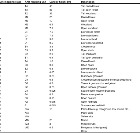
Table 3. Summary of vegetation mapping units

See Atlas of Australian Resources Volume 6 for details (AUSLIG 1990).

AAR mapping class AAR mapping unit Canopy height (m) Description

1 T4 40 Tall closed forest

2 T3 35 Tall open forest

3 T2 35 Tall woodland

4 M4 25 Closed forest

5 M3 10 Open forest

6 M2 0.5 Woodland

7 M1 7.5 Open woodland

8 L4 7.5 Low closed forest

9 L3 7.5 Low open forest

10 L2 3.0 Low woodland

11 L1 0.5 Low open woodland

12 S4 3.5 Closed shrub

13 S3 3.5 Open shrub

14 S2 2.0 Tall shrubland

15 S1 0.4 Tall open shrubland

16 Z4 1.0 Closed heath

17 Z3 0.8 Open heath

18 Z2 0.5 Low shrubland

19 Z1 0.05 Low open shrubland

20 H2 0.25 Hummock grassland

21 G4 0.5 Closed tussock grassland or closed sedgeland

22 G3 0.5 Tussock grassland or sedgeland

23 G2 0.25 Open tussock grassland

24 G1 0.025 Sparse open tussock grassland

25 F4 0.2 Dense sown pasture

26 F3 0.15 Sown pasture

27 F2 0.075 Open herbfield

28 F1 0.015 Sparse open herbfield

29 N/A 10 Paren lake (e.g. mangroves, low shrubs etc.)

30 N/A Peaty sand

31 N/A Saline lake

32 xM4 20 Mixed

33 xZ3 2 Mixed shrubs

34 dG3 0.5 Bluegrass (tufted grass)

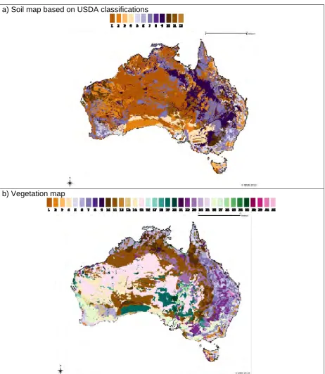
The soil-map classes used in Australia are shown in Figure 3a. Some soils are known to be

non-erodible (e.g. areas covered largely by bare rocks) and are excluded from the

calculations of wind erosion. The erodibilities of the rest of the soils are determined by the

threshold friction velocity, which is calculated in CEMSYS.

a) Soil map based on USDA classifications

b) Vegetation map

The vegetation type data in the GIS database provide a range of parameters such as

vegetation height, minimum vegetation stomatal resistance, vegetation albedo, etc. The

source of vegetation data is the

Atlas of Australian Resources

Volume 6 (AUSLIG 1990).

Vegetation is divided into 35 classes according to height, density and number of canopy

layers. The vegetation types for the Australian region are shown in Figure 3b.

The calculation of u

requires the frontal area index of roughness elements and the soil

moisture as inputs. The former is slowly varying with time and hence is assumed to be

constant for individual months and is updated monthly. In this study, frontal area index is

derived via an empirical relationship from a combination of satellite NDVI (Normalised

Differential Vegetation Index) data and GIS data for vegetation types.

The only new data incorporated into the model compared to previous publications using

CEMSYS was the NDVI data. Previously NDVI data has been used that was calculated from

the Advanced Very High Resolution Radiometer (AVHRR) Bpal series. Due to problems with

the Bpal data, this study used Moderate Resolution Imaging Spectroradiometer (MODIS)

NDVI data (MOD13Q1) at 16-day intervals derived from MODIS Land Products

(

) and further processed and distributed for

the Australian region via CSIRO Land and Water (Paget and King 2008). The CSIRO mosaic

NDVI archive and report can be accessed at

Monthly NDVI data from 2000–2008 were calculated from the 16-day NDVI time-series data

using the mean values. Abnormal values (e.g. null) were filled using neighbourhood values or

adjacent images using GIS focal function. Any negative NDVI values were set to zero. The

monthly NDVI data was resampled to the specific pixel size and dimensions required by the

CEMSYS model and then exported to ASCII grid format. Automated GIS programs were

developed to produce the required monthly NDVI and CEMSYS inputs.

Modelled CEMSYS six-hourly horizontal soil flux (TQ mg/m/s) data was averaged to give the

monthly data sets. TQ is representative of the wind erosion rate at a site, or in this case, the

average for the pixel. Pixel size was 50 x 50 km. CEMSYS can be run at a resolution of 10 x

10 km, as has been done for NSW.

2.2 DEVELOPING THE NRM REGIONAL MAP FOR WIND EROSION REPORTING

During the development of the wind erosion priority area maps for the 2009–10 Caring for

Our Country (C4oC) Business Plan (see

), the

2.3 CALCULATION OF STATISTICS

Statistics are presented at two time scales and three spatial scales. The time scales are:



Monthly (average of 6-hourly data), and



Dust-year (July to June) (average of monthly data).

The three spatial scales are:



continental



state, and



NRM

region.

ASCII model outputs from CEMSYS were imported into ArcGIS 9.3 and converted to

raster/grid files. These files were cookie-cut to 64 NRM regions, subregions, state and

national areas. The modelled monthly raster/grid data was then used to calculate the

percentage of each area within five erosion classes.

The monthly raster/grid data used the five-class system below.



Very Low (when TQ < 20 mg/m/s)



Low

(when TQ > 20–40 mg/m/s)



Moderate (when TQ > 40–160 mg/m/s)



High

(when TQ > 160–640 mg/m/s)



Very High (when TQ > 640 mg/m/s)

Different thresholds were applied to the dust-year data due to the longer averaging period;

that is a year vs. one month. The dust-year raster/grid data used the five-class system below.



Very Low (when TQ < 10 mg/m/s)



Low

(when TQ > 10–20 mg/m/s)



Moderate (when TQ > 20–80 mg/m/s)



High

(when TQ > 80–160 mg/m/s)



Very High (when TQ > 160 mg/m/s)

The threshold levels set for the erosion classifications for the 50 km pixel size were based on

previous experience with CEMSYS using 10 km pixel sizes. The classification thresholds

have been set using the 10 km data and the roadside survey (RoS) data from the Lower

Murray–Darling, Murray and Lachlan Catchment Management Authorities (CMAs) (Leys

et

al.

2009a). RoS data estimates erosion at a site using a five-class system:



Low

(no

erosion

evident)



Moderate (evidence of erosion but eroded sediment remains within the paddock)



High

(evidence that sediment is being exported off site)



Severe

(surface lowering of up to 10 cm)



Extreme

(surface lowering greater than 10 cm).

smaller than a 10-km pixel. Also, there can be several RoS sites with a range of erosion

values within a single 10-km pixel. Therefore, the approach was to set the threshold for the

modelled moderate erosion class proportional to the RoS moderate class results; that is, if

the RoS data indicated that 10% of the CMA area was in the moderate class, then the

threshold for the modelled moderate class was set to equal 10% of pixels for that CMA.

Due to the large pixel size of 50 km, it was difficult to use the RoS data to set the

classification thresholds as was done for the 10-km data. There is no equivalent Australian

monthly wind erosion data at any scale for testing the 50-km classifications. As such, these

classifications should be seen as a first step in the development of a robust classification

system.

3. Results

and

Discussion

CEMSYS is a modelling system that has gained acceptance via field testing (Shao

et al.

1996) and against dust events of short duration of three to four days (Shao

et al.

2007). To

date, CEMSYS has not been validated over longer time scales such as months and years as

presented here; therefore some caution must be used when interpreting this data. Despite

this, there is a ‘sensible’ distribution of erosion activity both in space and time. In this context

‘sensible’ is taken to mean that the extent and severity of the modelled erosion data

conforms to our knowledge of wind erosion. For example, we would expect the arid lands to

have higher levels of erosion than the humid lands and we would expect certain areas to

have erosion in summer and others in spring. These patterns are observed in the modelled

data.

Results are presented for two time scales and three spatial scales as listed below.

The time scales are:



Monthly (average of 6-hourly data), and



Dust-year (July to June) (average of monthly data).

The three spatial scales are:



continental



state, and



NRM

region.

3.1 MONTHLY DATA

The model output for the monthly data is displayed as maps for 2006–07 in Figure 5 and for

2007–08 in Figure 6. The statistics for each NRM region, state and national area are listed in

Appendix 2.

The occurrence of erosion is greatest just before the rainfall season, i.e. when ground cover

is generally lowest. In the northern parts of Australia, erosion commences before the wet

season in late spring/early summer. In the south of Australia, erosion commences in late

summer/early autumn.

If we define the erosion season as commencing when the high and very high classes exceed

5% of the nation within one month, then in 2006–07 the erosion season commenced in

October 2006 and finished in March 2007 (Figure 5). In 2007–08, the erosion season

commenced earlier in August 2007 and is high through to June 2008 with the exception of

May 2008 (Figure 6). The NRM regions with very high and high erosion during this period

are:



Queensland NRM regions of Desert Channels, South West, Border Rivers Maranoa–

Balonne, and Condamine



NSW regions of Western, Border Rivers–Gwydir, Namoi, Lachlan, Murrumbidgee, Murray

and Lower Murray–Darling



South Australian Arid Lands region



Northern Territory Pastoral and Non-pastoral regions, and

Wind erosion rate (mg/m/s)

Very High (>640) High (160-640) Moderate (40-160) Low (20-40) Very Low (<20)

Figure 5. Modelled monthly wind erosion maps for the period July 2006 to June 2007

Jul 2006

Aug 2006

Sep 2006

Oct 2006

Nov 2006

Dec2006

Jan 2007

Apr 2007

Jun 2007 Feb 2007

Mar 2007

Figure 6. Modelled monthly wind erosion maps for the period July 2007 to June 2008

Jul 2007

Aug 2007

Sep 2007

Oct 2007

Nov 2007

Dec2007

Jan 2008

Feb 2008

Mar 2008

Apr 2008

May 2008

Jun 2008

Wind erosion rate (mg/m/s)

Very High (>640)

High (160-640)

Moderate (40-160)

Low (20-40)

Other smaller regions also have high or very high erosion through the simulation period,

e.g. Northern and Southern Gulf in Queensland during July 2007 and North and South-east

of Tasmania during February and June 2008.

The months with the highest levels of erosion are December 2006 and October 2007 with

24% of pixels in the high and very high class. Peak erosion levels at the NRM level were in

November 2006 when the model predicted that the Desert Channels in Queensland had

96%, South West Queensland had 94% and Western NSW had 91% of their areas in the

high and very-high classes. These levels appear to be unrealistic which indicates that the

thresholds in the monthly five-class classification maybe set too low for northern NRM

regions. Another possible explanation lies in the use of the NDVI data to derive the frontal

area index (i.e. ground cover).

Previous studies (Lu

et al.

2001) have indicated that NDVI is not a good index for the

estimation of dead or senescent vegetation which can often form a large proportion of the

ground cover. When vegetation is dead the NDVI value is low and this results in a

correspondingly low frontal area index. As such the frontal area index is underestimated and

the erosion level is over estimated. We suspect that this underestimation of frontal index in

northern Australian grasslands in late spring occurs because the grass lands are covered in

dead or senescent cover that results in a low NDVI value. After the rains arrive in summer,

estimates are more realistic and we see a decline in erosion levels as seen in the ‘Desert

Channels’ region 17-monthly data in Appendix 2.

As pointed out in section 2.3, the monthly thresholds were based on previous CEMSYS

10-km data from NSW. From 2006 to 2008, there is CEMSYS modelled data at the 10-km

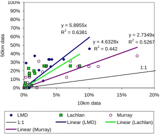
resolution for NSW. A comparison of the 10-km vs. 50-km data for the sum of the very high

and high erosion classes for the Lower Murray–Darling, Lachlan and Murray CMAs in NSW

is presented in Figure 7. The results show that for the percentage area of each CMA in the

high plus very high classes, the areas are three to six times higher for the 50-km results

compared to the 10-km results. This is most likely a function of scaling and is explained

below.

Understanding the operational concepts of the CEMSYS model helps explain the scaling

differences. Wind erosion is a complex process which depends on land cover, soil type, soil

moisture and wind conditions. Each of these dependences has significant spatial variability

across the Australian continent. In addition, both soil moisture and wind can be influenced by

local atmospheric conditions. Several researchers have identified this spatial variability as a

key issue in modelling wind erosion at continental and regional scales (Butler

et al.

2005,

Walker

et al.

2006, Reid

et al.

2008). To account for this variability, CEMSYS is run at two

scales (i.e. 50-km and 10-km scales).

In the initial run, atmospheric data from the United States’ National Oceanic and Atmospheric

Administration (NOAA) is used to calculate the wind speed and direction, surface

Figure 7. Comparison of 10-km and 50-km CEMSYS products for the percentage of the CMA

area in the high and very-high erosion classes

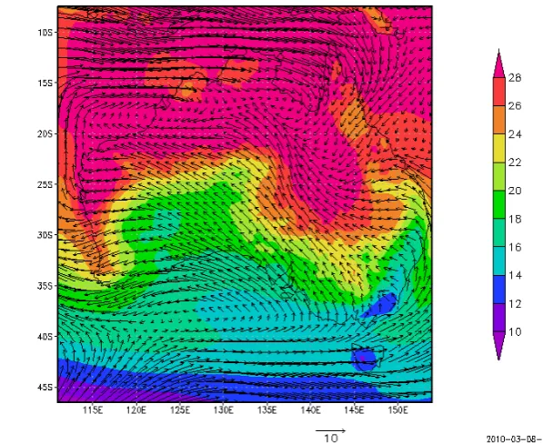
As Figures 8a and 9a show, the 50-km wind field does not show any localised wind effects,

thus the initial 50-km wind field just describes the general circulation pattern. To increase the

resolution of the model, a finer wind field is calculated using the initial 50-km data for use in

the 10-km model. The new 10-km wind field accounts for localised affects due to ranges etc.

as illustrated in Figures 8b and 9b. As wind erosivity varies with the cube of the wind speed,

these localised variations in wind speed can have a significant effect on wind erosion level

within each 50-km pixel.

Figure 8. Calculated monthly average wind fields (m/s) for February 2008 at 50-km resolution

(a) and 10-km resolution (b).

y = 5.8955x

R

= 0.6381

y = 4.6328x

R

= 0.442

y = 2.7349x

R

= 0.5267

0%

10%

20%

30%

40%

50%

60%

70%

80%

90%

100%

0%

5%

10%

15%

20%

10km data

50k

m d

ata

LMD

Lachlan

Murray

1:1

Linear (LMD)

Linear (Lachlan)

Linear (Murray)

Figure 9. Contour maps illustrating the spatial variability in wind speed (m/s) for February 2008

at 50-km (a) and 10-km (b) resolutions

In addition, the percentage composition of erodibility land types within each of the 10-km

pixels can be significantly different from each other and the overlying 50-km pixel. As stated

by McTainsh

et al.

(1996) and Butler

et al.

(2005), small variability in the percentage of

erodible land types can have a significant impact on the soil erodibility calculations. The

McTainsh

et al.

(1996) study looked at three erodibility scenarios within the Channel Country

of western Queensland. Scenario 1 assumed that the three main land types were eroding at

uniform rates; Scenario 2 assumed that the three land types were eroding at different rates;

while Scenario 3 assumed that the area of dunes was increased by 5%, while the area of

alluvium decreased by 5% in comparison to Scenario 2. Table 4 shows the results of this

study.

Table 4 Estimated soil loss rates in t/km

under three erodibility scenarios in the Channel

Country of western Queensland

Source: McTainsh et al. (1996).

Scenario 1 Scenario 2 Scenario 3

Land type (t/km2_{) (t/km}2_{) (t/km}2₎

Dunes 389.2 124.4

Alluvium 38.1 151.2 208.8

Downs 1.9 1.9

Two significant results from this study are relevant to this report. The first is that each land

type within a pixel can be eroding at significantly different rates. Secondly, a small change in

percentage composition of the pixels can result in a significant change in the overall

erodibility. Thus, the variability in the composition of the pixels, when combined with localised

changes in wind field, are the most likely reasons for the differences observed in the 50-km

and 10-km data. This scaling issue is well documented (Walker

et al.

2006, Reid

et al.

2008)

and indicates the importance of comparing data of like scales.

Currently the 10-km data is being validated against the NSW DustWatch Node data which

has 26 stations with dust concentration at 1-hour resolution. This will provide information on

the accuracy of the 10-km data, and may suggest ways to improve the 50-km data.

3.2 ANNUAL DUST-YEAR DATA

There are differences in the spatial distribution of the 2006–07 and 2007–08 dust-years

(Figure 10). The full annual statistical data is presented in Appendix 3. If we consider only the

high and very high classes within each NRM region as the percentage of the NRM with

erosion levels of concern, then there are several NRM regions that reached this level in

either of the two years and they are listed in Table 5. Due to the low sample number of

individual months (e.g. only two January readings) there is not adequate data to determine

statistical differences between individual months. However if we treat the months as

replicates within a dust storm year (DSY) then preliminary annual comparisons are

statistically possible. The underlying assumption for the paired t-test with equality of means is

that the months are replicates; however, in this case we know there is a season variation of

erosion through the year and so this assumption is not up held. Despite that the t-test data is

presented in Table 5. The results indicate that only six NRM regions were statistically

different (

P

<0.05) between DSY 06-07 and 07-08 and that there were no statistical

Table 5. National, state and NRM monthly percentages of high and very high class erosion

Month Year Nati

onal NT WA SA Qld Vic NSW NT Arid Centre-Pastoral (r13)

Gascoyne Murchison (r15)

Desert Channels (r17)

Goldfields Nullarbor (r19)

South West Queensland (r23)

S.A. Arid Lands (r26)

Western (r32)

Namoi (r33)

Lower Murray Darling (r40)

Lachlan (r42)

Murray (r50)

Jul-06 0607 0 0 0 1 0 0 0 0 0 0 1 1 2 0 0 0 0 0

Aug-06 0607 0 0 0 0 1 0 0 0 0 1 0 0 0 0 0 0 0 0

Sep-06 0607 2 0 2 2 3 0 0 0 0 7 3 1 5 1 0 0 0 0

Oct-06 0607 7 2 4 13 13 0 5 3 0 40 7 16 26 18 0 0 0 0

Nov-06 0607 21 4 5 30 47 1 43 10 0 96 7 94 58 91 53 38 23 31

Dec-06 0607 24 13 16 35 36 1 30 26 2 92 25 79 62 76 13 33 20 31

Jan-07 0607 17 5 12 32 23 1 27 9 1 64 17 46 59 75 7 21 14 25

Feb-07 0607 6 0 5 10 4 1 14 1 0 13 7 3 20 47 0 0 3 19

Mar-07 0607 18 7 20 32 13 1 27 11 15 39 27 22 62 75 7 29 17 25

Apr-07 0607 4 0 1 9 3 0 16 0 0 6 1 11 18 57 0 0 0 0

May-07 0607 2 0 1 7 2 0 6 0 1 7 1 1 14 21 0 0 0 6

Jun-07 0607 4 0 5 1 5 0 15 0 9 3 5 7 2 45 13 8 3 13

Jul-07 0708 1 0 0 2 1 0 0 0 1 1 0 0 3 0 0 0 0 0

Aug-07 0708 5 3 6 3 8 0 0 8 15 26 6 0 6 0 0 0 0 0

Sep-07 0708 12 3 1 30 19 0 23 8 1 63 2 11 60 60 0 33 26 0

Oct-07 0708 24 10 18 39 36 0 32 26 10 85 25 59 67 75 27 33 26 25

Nov-07 0708 20 10 17 35 26 1 20 26 16 74 23 9 60 47 0 25 26 25

Dec-07 0708 15 5 14 28 17 1 21 14 0 56 16 13 52 54 0 8 26 26

Jan-08 0708 17 5 19 38 12 1 24 12 0 41 24 9 66 49 0 46 25 38

Feb-08 0708 14 6 13 30 11 1 16 15 0 37 16 7 56 35 0 33 17 13

Mar-08 0708 5 1 5 13 7 0 3 2 0 24 3 0 26 8 0 0 3 13

Apr-08 0708 7 4 0 15 13 0 10 12 0 42 0 13 29 32 13 0 6 0

May-08 0708 2 2 0 3 4 0 1 6 0 11 0 0 5 4 0 0 0 0

Jun-08 0708 8 13 7 1 15 0 0 36 18 39 6 0 2 0 0 0 0 0

Mean 0607 8.8 2.6 5.9 14.3 12.5 0.4 15.3 5.0 2.3 30.7 8.4 23.4 27.3 42.2 7.8 10.8 6.7 12.5

Stdev 8.7 4.1 6.6 13.9 15.3 0.5 14.0 7.9 4.7 35.6 9.4 32.4 25.6 33.3 15.1 15.1 9.0 13.0

Mean 0708 10.8 5.2 8.3 19.8 14.1 0.3 12.5 13.8 5.1 41.6 10.1 10.1 36.0 30.3 3.3 14.8 12.9 11.7

Stdev 7.3 4.0 7.5 15.1 9.7 0.5 11.5 10.7 7.4 24.8 10.0 16.3 26.8 27.0 8.3 17.7 12.3 13.7

Month Year NT Non Pastoral (r14) BR Maranoa- Balonne (r24)

Condamine (r28)

Northern Agricultural (r29)

Border rivers-Gwydir (r31)

Avon (r34)

Northern and Yorke (r39)

Murrumbidgee (r46)

Jul-06 0607 0 0 0 0 0 0 0 0

Aug-06 0607 0 0 0 0 0 0 0 0

Sep-06 0607 0 0 0 0 0 0 0 0

Oct-06 0607 3 0 0 0 0 0 0 0

Nov-06 0607 2 54 100 7 66 13 10 8

Dec-06 0607 15 5 0 6 10 18 10 8

Jan-07 0607 8 3 0 7 0 24 0 4

Feb-07 0607 1 3 0 6 0 28 0 0

Mar-07 0607 15 3 0 7 0 24 10 4

Apr-07 0607 0 0 0 3 0 11 0 0

May-07 0607 0 0 0 0 0 0 0 0

Jun-07 0607 0 17 60 7 0 0 0 0

Jul-07 0708 0 0 0 3 0 0 0 0

Aug-07 0708 0 0 0 0 0 0 0 0

Sep-07 0708 0 0 0 3 0 0 19 8

Oct-07 0708 0 5 0 13 5 16 29 19

Nov-07 0708 0 0 0 13 0 13 24 12

Dec-07 0708 0 0 0 40 0 67 10 12

Jan-08 0708 0 0 0 40 0 80 29 19

Feb-08 0708 0 0 0 50 0 60 19 8

Mar-08 0708 0 0 0 26 0 47 5 0

Apr-08 0708 0 0 0 0 0 0 10 0

May-08 0708 0 0 0 0 0 0 5 0

Jun-08 0708 0 0 0 3 0 0 5 0

Mean 0607 3.7 7.1 13.3 3.6 6.3 9.8 2.5 2.0

Stdev 5.8 15.5 32.3 3.3 19.0 11.2 4.5 3.2

Mean 0708 0.0 0.4 0.0 15.9 0.4 23.6 12.9 6.5

Stdev 0.0 1.4 0.0 18.3 1.4 30.8 10.7 7.6

The differences in erosion levels between the 2006–07 and 2007–08 dust-years for the NRM

regions were as follows.



Queensland regions: Desert Channels increased from 31 to 42%, South West decreased

from 23 to 10%, Border Rivers Maranoa-Balonne decreased from 7 to 0.5% and

Condamine 13 to 0%.



NSW regions: Lower Murray Darling increased from 11 to 15%, Lachlan 7 to 13%,

Murrumbidgee 2 to 7% (significantly different) and Western decreased from 42 to 30%,

Murray 13 to 12%, Border Rivers Gwydir 6 to 1% and Namoi from 8 to 3 %.



South Australian regions: Arid Lands increased from 27 to 36%, and Northern and Yorke

increased from 2 to 13 % (significantly different).



Northern Territory regions: NT Arid Centre Pastoral increased from 5 to 14% (significantly

different) and NT Non Pastoral decreased from 4 to 0% (significantly different).



Western Australia: Gascoyne Murchison increased for 2 to 5%, Goldfields Nullarbor 8 to

10%, Northern Agricultural from 4 to 16% (significantly different) and Avon 10 to 24%

(significantly different).

At a state scale, South Australia increased its percentage area in 2006–07 to 2007–08 from

14 to 20%, Queensland increased from 12 to 14%, NSW decreased from 15 to 12% and the

Northern Territory increased from 6 to 8%.

Nationally, 2007–08 had higher erosion levels of 11%, compared to 2006–07 with 9% (not

significantly different

Error! Reference source not found.

).

NRM regions with erosion level of concern (high and very classes) tend to be focused in arid

and semi-arid rangelands and the agricultural (farming) land in parts of South Australia and

Western Australia. The non-agricultural lands of western South Australia, northern Northern

Territory and eastern Western Australia all have low erosion levels.

Rainfall is a key driver of wind erosion. The rainfall data in Figure 11 shows that as the

Northern Territory, Queensland and South Australia dried out in 2007–08, they experienced

increased erosion, although not as much as one might expect for the Northern Territory,

which had low levels of erosion despite the very much below average rainfall. Interestingly,

the relationships in NSW and Western Australia are not so obvious. Areas with average

rainfall in NSW had erosion predicted, and areas with very much below average rainfall in

Western Australia had little erosion predicted. One explanation could be the timing of the

rainfall and high wind events. For example, rainfall just before a high wind event would result

in lower erosion rates. Another explanation is land management effects that can decrease or

accelerate erosion levels.

Another feature of the modelling is that at the yearly and monthly time scales there is a lack

of erosion predicted for the cropping areas in the Mallee landscapes of north-western Victoria

and South Australia and NRM regions in the drier cropping areas of Western Australia. We

suspect this is related to known issues with the soils data used in CEMSYS and the use of

NDVI to derive the cover fraction. These limitations appear to be leading to underestimation

of the erosion in these agricultural areas. The solution lies in improving the soils and ground

cover data as recommended in the Leys report (Leys

et al.

2009b).

C4oC has funded projects such as the ‘Wind Erosion Histories, Model Input Data and

Community DustWatch’ project (McTainsh

et al.

2010) to improve the soil particle data used

in CEMSYS. The soil particle-size data is not the standard four-class data derived from most

soil surveys; rather it is 256-class data of soils that are analysed after being minimally and

fully dispersed (McTainsh

et al.

2010). This special analysis is the reason for the specific

funding for soil particle analysis. C4oC is also in the process of funding a project to provide

fractional ground cover data (TERN, AusCover project) that should provide better estimates

than the current NDVI method. These investments will assist in improving the modelling once

the results are available and have been incorporated into the model.

Despite these limitations, CEMSYS appears to provide information on the spatial and

temporal trends of erosion in Australia and at the state and NRM regional level. The only

other data available at the national scale to compare the CEMSYS data against is the Dust

Storm Index (DSI) (McTainsh 1998). DSI is based on the annual frequency and intensity of

dust visibility reduction at 110 Bureau of Meteorology (BoM) sites (Figure 12).

There are obvious methodological differences between the two products. CEMSYS

estimates erosion for every pixel (2,891 for Australia) and DSI reports a dust level at 110

BoM sites (Figure 12) and then extrapolates the intervening areas using nearest-neighbour

fitting. When comparing the two methods it is important to note that if DSI reports dust then

there should be erosion calculated by upwind of where it was measured with DSI.

Conversely if CEMSYS does predict erosion and DSI does not measure dust, this could be

due to the fact that there maybe no BoM stations in that area or no observation was made at

the time of day dustpassed. Considering the differences and scales of the two methods,

there is general agreement (Figure 13) which gives us confidence in the CEMSYS and the

DSI data.

The CEMSYS results offer greater resolution in the rangeland areas due to the reduced

number of sites the BoM has to record visibility data. For example, in region 21 (NT Arid

Centre Simpson) DSI maps this region as high erosion. This is because DSI extrapolates

between Alice Springs and Birdsville (Figure 12). Conversely, CEMSYS predicts very low

erosion in region 21 which is more likely because this is area is not used for extensive

grazing and tends to have an adequate vegetation level to control the erosion and this is

predicted by CEMSYS. If a BoM station was located in the Simpson Desert, then the DSI

prediction would be more accurate. Similarly the West Australian Rangelands have few BoM

stations and there appears to be more detail in this region with CEMSYS.

4. CEMSYS Implementation Plan

4.1 BACKGROUND

This section outlines a way of implementing national wind erosion modelling using CEMSYS

at a finer scale (10-km grid). This was one of the recommendations of the Leys report (Leys

et al.

2009b, p. xii). It stated that a four-year project should be done that provided:

Annual modelled wind erosion maps (2000 to present) suitable for use at national and

state scales identifying which areas are affected by wind erosion and the severity of this

problem. These will help target future investments and provide trends in erosion at NRM

regional level ($150K p.a.).

The 50-km grid data presented here has proven useful at the national and state scale, but

the coarse scale limits its application to smaller NRM regions and those with more complex

landscapes.

CEMSYS has been applied at 10-km resolution in NSW (and the northern part of Victoria)

since June 2006. Several inland NSW CMAs (Lower Murray–Darling, Lachlan and Murray)

have contributed to the funding of this work for their monitoring and evaluation programs.

Figure 14 shows the improved output for NSW for 2007–08. The 10-km data shows greater

detail and allows for the identification of landscape features with higher erosion levels, such

as the Barrier and Grey Ranges in western NSW. Another example is the scalded river

margins along the Edward and Wakool Rivers in the western end of the Murray CMA which

are classified High and Very High with the 10-km data and Low and Moderate with the 50-km

data. The 10-km data makes it clearer that it is the river margins and not the whole of the

western end of the CMA that would benefit from investment.

4.2 PROPOSED IMPROVEMENTS

The study has identified a number of possible limitations to the CEMSYS modelling that

should be improved. These include:

1. Incorporation of the updated soil particle-size analysis for all representative soil types

used in CEMSYS. These model runs were done with five fully dispersed soils

representing the Australian continent, a vast simplicity. Through the MERI C4oC

2008–09 funding a further 19 soils will become available and there is a need to

incorporate them into the model. Note that the particle-size analysis is a 256-class

analysis of samples that are pre-treated in minimally and fully dispersed states.

2. Use of a consistent NDVI record. Over the years that CEMSYS has been run, various

NDVI data sources have been employed. Each of these is slightly different (e.g.

AVHRR, SeaWiFs, and MODIS). In 2008–09, CSIRO made available the MODIS

NDVI data (MOD13Q1) 16-day interval product for the period 2000 to the current

date. So that all years can be compared, we propose to use this consistent product at

the 50-km CEMSYS resolution for the 2000 to 2011 period should the implementation

plan be funded. This extended data record would give a better indication of the

performance of CEMSYS because it could be compared to the DSI for this period and

allow us to gain a better understanding of the ranges of wind erosion intensity under

climatic extremes.

3. The use of NDVI to calculate the cover fraction has been shown to be unreliable

because NDVI is a greenness index and fails to adequately address the bleached or

dead cover that is present. The currently funded TERN/AusCover project is most

likely to deliver a MODIS 500-m resolution fractional cover product that has a bare

ground component. If this is product is delivered, it is proposed to use this rather than

the MODIS NDVI product outlined in point 2 above.

4. A major anomaly is the failure to identify erosion in known wind erosion regions such

as the Mallee of north-western Victoria and southern NSW and the farming areas in

Western Australia and South Australia. If the improvements in points 1 and 2 above

do not address this issue, then the operational scale of the model might need to be

considered for some areas, that is, from 10-km to 1-km resolution. This would be a

major undertaking as it means we would need to address the atmospheric resolution

and the soil data resolution.

5. Once the improved input data are available, a significant part of the project would be

to test the new model against DSI and DustWatch Node data to see if the model has

improved.

6. Delivery of a 10-km product for Australia. This would require several domains to be

run through the model. The 10-km domains would be:

f) Southern Western Australia

g) Northern Western Australia

The proposed task is not a simple one and will take considerable computing time to

complete. The twelve monthly maps at 50-km resolution are less complex and take about

one month to complete. It will take about one month to produce a single monthly continental

map for the seven 10-km domains using the current computing facilities at USQ. With the

installation of a new high performance computing facility at USQ, this time should be

significantly reduced once this facility becomes operational. This computational increase is

related to needing to recalculate atmospheric and soil conditions within each 10-km pixel to

account for localised effects (i.e. soil moisture and wind field variations). There are also

research issues about the best methods to combine the seven domains into one map.

4.3 PROPOSED PRODUCTS

If this implementation plan is funded for four years then the proposed products would be:



Monthly and dust-year maps at 50-km resolution for the period 2000 to 2011, and



Monthly and dust-year maps at 10-km resolution for at least three years.

Figure 15 shows a combination of the two products: 50-km resolution for all states except

NSW at 10-km resolution.

4.4 COSTING

CEMSYS is currently run at USQ under the direction of Dr Harry Butler. Dr Butler is on the

teaching staff and has limited ability to undertake this modelling full time unless a

replacement staff member is employed to take on his teaching work. USQ has agreed in

principal to letting Dr Butler undertake the modelling if funding for his salary and computer

operational costs can be provided for four years. In-kind support in the form of computing

facilities and administrative support can be offered. An estimate of $130,000 p.a. has been

suggested by USQ.

The project will be managed by Dr Leys at DECCW and will involve two other DECCW staff

who will provide GIS and statistical analysis support to complete the project. Their time can

be offered as in-kind support and a modest travel budget for meetings and field validation of

model outputs and computer consumables component is requested at $20,000 p.a.

5. Conclusions

Both objectives of this project have been successfully completed; that is, the development of

a) monthly and annual maps and statistics of wind erosion at 50-km resolution for two years,

and b) an implementation plan for the provision of a longer time series of low-resolution

maps and three years of higher resolution maps for all of Australia.

Monthly and dust-year maps and statistics of wind erosion as measured by horizontal sand

flux (TQ mg/m/s) from the CEMSYS model for the period July 2006 to June 2007 were

produced to describe the intensity of wind erosion for Australia, the states and NRM regions.

The model results indicated monthly and yearly variations. The erosion seasons, defined as

when the high and very high classes of erosion exceed 5% of the nation, commenced in

October 2006 and finished in March 2007 and recommenced in August 2007 and remained

high through to June 2008 with the exception of May 2008.The NRM regions with very high

and high erosion during this period were



in Queensland: Desert Channels, South West, Border Rivers Maranoa–Balonne, and

Condamine



in NSW: Western, Border Rivers–Gwydir, Namoi, Lachlan, Murrumbidgee, Murray and

Lower Murray–Darling regions



in South Australia: the Arid Lands and Northern and Yorke regions



in the Northern Territory: the Pastoral and Non-Pastoral regions, and



in Western Australian: the Rangeland regions of the Goldfields Nullarbor and Gascoyne

Murchison, Northern Agricultural and the Avon region.

NRM regions with erosion levels of concern (high and very classes) tend to be focused in

arid and semi-arid rangelands and the agricultural (farming) land in parts of South Australia

and Western Australia. The non-agricultural lands of western South Australia, northern

Northern Territory and eastern Western Australia all have low erosion levels.

At the state scale, South Australia had the highest percentage of area in the high and very

high class with 14 to 20% respectively in 2006–07 and 2007–08. Queensland was the

second highest state with 13 to 14%, followed by NSW with 15 to 13% and the Northern

Territory with 3 to 5%.

Nationally 2007–08 had greater percentage of eroding areas with 11% compared to 9% in

2006–07.

There is a lack of data to test the CEMSYS output against at the 50- and 10-km scales.

Specifically data that details the intensity of erosion (sand flux) at a site is required. Roadside

survey (RoS) data is the best data available but there are difficulties with the scale

differences (RoS 1-ha scale) vs. the 50 and 10-km modelling scales. Despite these scale

differences the RoS data was used to establish the erosion class thresholds. As more RoS

data becomes available from future surveys and other states it will offer a new test data

source. Until then the only other data available is visibility reduction data used in the Dust

Storm Index (DSI).

there was generally good agreement. However, the CEMSYS data offers greater spatial

resolution, especially in the rangelands where there are fewer Bureau of Meteorology

stations to record the visibility data that the DSI uses. The DSI still has the advantage of a

longer time series from 1960 to the present.

This study highlights some of the problems with scaling and indicates that comparison of

products derived at different scales is very problematic. Finer scale products have the

advantage of being able to more accurately represent landscape features such as rivers or

hills, have a greater chance of reporting a greater range of values due to the heterogeneous

nature of landscapes and provide greater numbers of pixels for statistical analysis.

There are major advantages for providing a longer time scale (2000 to current) and

6. References

AUSLIG (1990) 'Atlas of Australian Resources, Vol 6: Vegetation and Land Information.'

(Vegetation Surveying and Land Information Group, Department of Administrative

Services: Canberra)

Butler, H., G. McTainsh, W. Hogarth, and Leys, J. (2005), Kinky profiles: effects of soil

surface heating upon vertical dust concentration profiles in the Channel Country of

Western Queensland, Australia, Journal of Geophysical Research - Earth Surface,

110(F04025), doi:10.1029/2004JF000272.

Butler H, Shao Y, Leys J, McTainsh G (2008). Modelling wind erosion at national and

regional scale using the CEMSYS model. National Land and Water Resources Audit,

Canberra, ACT. 37 pp.

Irannejad, P., and Shao, Y. (1998). Description and validation of the

Atmosphere-Land-Surface Interaction Scheme (ALSIS) with HAPEX and Cabauw data.

Global Planet

Change

,

19

, 87-114.

Leslie, L. M., and Wightwick, G. R. (1995). A new limited-area numerical weather prediction

model for operations and research: formulation and assessment. Monthly Weather

Review, 123, 1759-1775.

Leys J, Heidenreich S, Murphy S, Koen T, Biesaga K, Yang X (2009a). Lower Murray

Darling CMA Catchment Report Card - Wind Erosion 2007-09. Department of

Environment, Climate Change and Water, Sydney. 40 pp.

Leys, J., Smith, J., MacRae, C., Rickards, J., Yang, X., Randall, L., Hairsine, P., Dixon, J.,

and McTainsh, G. (2009b). Improving the Capacity to Monitor Wind and Water Erosion: A

Review. Department of Agriculture, Fisheries and Forests, Australian Government,

Canberra. 160 pp.

Lu, H., Raupach, M.R., and McVicar, T.R. (2001). Decomposition of vegetation cover into

woody and herbaceous components using AVHRR NDVI time series. CSIRO Land and

Water Technical Report. No. 35/01. CSIRO, Canberra. 38 pp.

McTainsh, G. H. (1998). Dust Storm Index. In Sustainable Agriculture: assessing Australia's

recent performance. SCARM Report. No. 70. Standing Committee on Agriculture and

Resource Management, Canberra. 55-62 pp.

McTainsh, G., J. Leys, W. Nickling, and Lynch, A. (1996). Sediment loads, source areas and

soil loss rates during a large dust storm in the Queensland Channel Country, Lake Eyre

Basin. Australian Rangelands Conference, Port Pirie, South Australia.

McTainish, G., Strong, C., Leys, J., Baker, M., Tews, K., and Barton, K. (2010). Wind Erosion

Histories, Model Input Data and Community DustWatch. Atmospheric Environment

Research Centre, Griffith University, Brisbane. 358 pp.

NATMAP (1980) 'Atlas of Australian Resources, Vol 3: Soils and Land Use.' Division of

National Mapping, Department of National Development, Canberra.

Marine and Atmospheric Research. Internal Report 004.

Reid, J., E. Reid, A. Walker, S. Piketh, S. Cliff, A. Al Mandoos, S. Tsay, and Eck, T. (2008).

Dynamics of southwest Asian dust particle size characteristics with implications for global

dust research, Journal Geophysical Research-Atmosphere, 113(D14), D14212.

Shao, Y. (2003). Real-time numerical prediction of northeast Asian dust storms using an

integrated modelling system. Journal of Geophysical Research, 108, 4691

10.1029/2003JD003667.

Shao, Y., and Leslie, L. M. (1997). Wind erosion prediction over the Australian continent.

Journal of Geophysical Research, 102(D25), 30,091-30,105.

Shao, Y., Leys, J., McTainsh, G. and Tews, K. (2007). Numerical simulation of the October

2002 dust event in Australia. Journal of Geophysical Research, 112, 1-12.

Shao, Y., and Lu, H. (2000). A simple expression for wind erosion threshold friction velocity.

Journal of Geophysical Research, 102, 30091-30105.

Shao, Y., Raupach, M. R., and Leys, J. F. (1996). A model for predicting aeolian sand drift

and dust entrainment on scales from paddock to region. Australian Journal of Soil

Research, 34(3), 309-342.

Appendix 1: NRM regions and sub regions

SORTED BY REGION NUMBER

Region Number in

Figure 1

Region Name State

1 Torres Strait Queensland

2 Cape York Queensland

3 NT - Top End Northern Territory

4 NT - Melville Island Northern Territory

5 NT - Darwin Northern Territory

6 NT - Katherine-Douglas Northern Territory

7 Rangelands - Kimberley Western Australia

8 NT - Savannah Northern Territory

9 NT - Victoria River Northern Territory

10 Northern Gulf Queensland

11 Wet Tropics Queensland

12 Southern Gulf Queensland

13 NT - Arid Centre - Pastoral Northern Territory

14 NT - Arid Centre - Non Pastoral Northern Territory

15 Rangelands - Gascoyne Murchison Western Australia

16 Burdekin Queensland

17 Desert Channels Queensland

18 Mackay Whitsunday Queensland

19 Rangelands - Goldfields Nullarbor Western Australia

20 Fitzroy Queensland

21 NT - Arid Centre Simpson Northern Territory

22 Burnett Mary Queensland

23 South West Queensland Queensland

24 Border Rivers Maranoa - Balonne Queensland

25 South East Queensland Queensland

26 South Australian Arid Lands South Australia

27 Alinytjara Wilurara South Australia

28 Condamine Queensland

29 Northern Agricultural Western Australia

30 Northern Rivers New South Wales

31 Border Rivers-Gwydir New South Wales

32 Western New South Wales

33 Namoi New South Wales

34 Avon Western Australia

35 Central West New South Wales

36 Swan Western Australia

37 Eyre Peninsula South Australia

38 Hunter-Central Rivers New South Wales

39 Northern and Yorke South Australia

40 Lower Murray Darling New South Wales

41 South West Western Australia

43 South Australian Murray Darling Basin South Australia

44 South Coast Western Australia

45 Hawkesbury-Nepean New South Wales

46 Murrumbidgee New South Wales

47 Mallee Victoria

48 Southern Rivers New South Wales

49 Adelaide and Mount Lofty Ranges South Australia

50 Murray New South Wales

51 North Central Victoria

52 Kangaroo Island South Australia

53 South East South Australia

54 Wimmera Victoria

55 Goulburn Broken Victoria

56 North East Victoria

57 East Gippsland Victoria

58 Glenelg Hopkins Victoria

59 West Gippsland Victoria

60 Port Phillip and Westernport Victoria

61 Corangamite Victoria

62 Tas - Flinders Tasmania

63 Tas - North West Tasmania

64 Tas - North Tasmania

65 Tas - South East Tasmania

SORTED BY REGION NAME

Region Number in

Figure 1

Region Name State

49 Adelaide and Mount Lofty Ranges South Australia

27 Alinytjara Wilurara South Australia

34 Avon Western Australia

31 Border Rivers-Gwydir New South Wales

24 Border Rivers Maranoa - Balonne Queensland

16 Burdekin Queensland

22 Burnett Mary Queensland

2 Cape York Queensland

35 Central West New South Wales

28 Condamine Queensland

61 Corangamite Victoria

17 Desert Channels