Scientific Data Mining for
Spatio-Temporal Hydroacoustic Data Sets
Bart Buelens
Submitted in fulfilment of the requirements for the Degree of
Doctor of Philosophy
Declaration
This thesis contains no material which has been accepted for the award of any other higher degree or graduate diploma in any tertiary institution. To the best of my knowledge and belief, this thesis contains no material previously published or written by another person, except where due reference has been made in the text of the thesis, nor does this thesis contain any material that infringes copyright.
the date this statement was signed. Following that time the thesis may be made available for loan and limited copying in accordance with the Copyright Act 1968.
Bart Buelens
Statement of co-authorship
The publications of the work undertaken as part of this thesis are the following: Buelens, B., Williams, R., Sale, A., and Pauly, T. (2003). "Midwater acoustic modeling for multibeam sonar simulation," 146th ASA Meeting (Austin, Texas), The Journal of the Acoustical Society of America 114, p. 2308.
Buelens, B., Williams, R., Sale, A., and Pauly, T. (2004). "A framework for scientific data mining in hydroacoustic data sets," 2nd International Conference on Artificial Intelligence in Science and Technology (AISAT) (Hobart, Tasmania, Australia), pp. 104-108.
Buelens, B., Williams, R., Sale, A., and Pauly, T. (2005). "Model inversion for midwater multibeam backscatter data analysis," IEEE Oceans '05 Europe (Brest, France), pp. 431-435.
Buelens, B., Williams, R., Sale, A., and Pauly, T. (2005). "A scientific data mining approach to midwater multibeam echosounding for fisheries applications," 1st International Conference on Underwater Acoustic Measurements: Technologies & Results (UAM) (Heraklion, Crete, Greece).
Buelens, B., Williams, R., Sale, A., and Pauly, T. (2006). "Computational challenges in processing and analysis of full-watercolumn multibeam sonar data," 8th European Conference on Underwater Acoustics, edited by S. M. Jesus, and 0. C. Rodriguez (Carvoeiro, Portugal), pp. 799-804.
Buelens, B., Pauly, T., Williams, R., and Sale, A. (in press). "Kernel methods for detection and classification of fish schools in single beam and multibeam acoustic data," in ICES Journal of Marine Science, Special Issue on the Ecosystem Approach with Fisheries Acoustics and Complementary Technologies.
The proportion of the work undertaken for each of the manuscripts is as follows: • Mr. Bart Buelens (70%) is the primary author. He conducted the research
and prepared the material for publication.
• Dr. Tim Pauly (10%) of Myriax Pty Ltd contributed to aspects relating to underwater acoustics and fisheries research and offered comments on manuscript drafts.
We the undersigned agree with the above stated proportion of work undertaken for each of the above published or submitted manuscripts contributing to this
thesis.
Signed:
Date:
Dr. Ray Williams Supervisor
School of Computing and Information Systems University of Tasmania
/ to 0
Dr. Julian Dermoudy Head of School
School of Computing and Information Systems University of Tasmania
Abstract
Managing natural marine resources for sustainable exploitation of the oceans and the flora and fauna they contain is a challenging task. Decisions by policy makers are based on advice from the scientific community. Through surveying and monitoring programs, scientists study the marine environment to gain insight into its structure and function. Employing acoustic techniques, sonar systems are often the best tools available to effectively observe aquatic environments. Important applications include fisheries and seafloor mapping. Fish stock assessments are typically conducted using single beam echosounders, while bathymetric surveys are conducted with multibeam sonar.
Multibeam sonar instruments that are capable of collecting samples for the complete water column are an emerging technology. Since they collect acoustic data over much greater sampling volumes than single beam instruments, significant improvements in fisheries studies are expected. The combined collection of seafloor and water-column data will lead to survey cost savings and to an integrated, ecosystem-based approach to monitoring the ocean environment. While standard data analysis procedures are established for single beam fisheries and standard multibeam bathymetric applications, this is not the case for full water-column multibeam sonar data.
In this thesis, a data mining approach for handling such data is proposed. The developed method consists of a preprocessing algorithm based on an inversion technique, followed by a pattern analysis algorithm using kernel clustering methods. The preprocessing algorithm applies a deconvolution as a model inversion method to reduce the data set in size and to convert the acoustic measurements into a generic vector representation. Each vector has a spatial and a temporal component as well as a number of additional features typically relating to the acoustic backscatter energy. These spatio-temporal vectors are then subjected to pattern analysis algorithms. Two clustering algorithms are selected: a density based spatial clustering algorithm, and a clustering algorithm based on kernel methods. A new method is developed to allow the kernel clustering algorithm to make use of the spatial and non-spatial components of the data in a combined fashion. This results in a powerful, flexible and versatile clustering procedure. The outcome is a segmentation of the data into coherent structures, for example fish schools and the seabed. Classification is achieved through the differentiation between data clusters indicative of different fish species or seabed habitats. The effectiveness of the data mining methods is demonstrated in a number of case studies.
I am very grateful to my supervisors Ray Williams and Arthur Sale at the University, and Tim Pauly at Myriax Pty Ltd, for the support they have given me during the six years of candidature. They have been very responsive to questions, provided me with useful advice and feedback, and have shown a great interest in my project. I appreciate the effort they have put in maintaining their supervisory roles also while I was overseas during the last two years of candidature.
I wish to thank Myriax Pty Ltd (formerly known as SonarData Pty Ltd) for providing the funding for my PhD project. Such an investment carries a certain level of risk and I am grateful that they have put their trust in me.
The feedback I received from Matt Wilson, David Millington and Toby Jarvis who have proof read my thesis has been very valuable, for which I am thankful.
The following people have provided me with sonar data sets that I could use in the context of my PhD research: John Anderson, Northwest Atlantic Fisheries Centre, Department of Fisheries and Oceans, St John's, NF, Canada; Ken Foote and Dezhuang Chu from Woods Hole Oceanographic Institution, Woods Hole, MA, USA; John Home, School of Fisheries, University of Washington, Seattle, WA, USA; Toby Jarvis, Australian Antarctic Division, Kingston, Tasmania, Australia; Chris Malzone, Reson Inc., Goleta, CA, USA; Tom Weber, University of New Hampshire, Center for Coastal and Ocean Mapping, Durham, NH, USA. I appreciate their efforts in making the data files available. Where such data files are used in examples or case studies in this thesis, the source of the data is acknowledged in the text.
Finally I thank my wife Lieve for giving me the time and space to pursue this PhD, and generally for putting up with me in particular during the more stressful stages of candidature. Siska-Lut and Komeel, my two children, were born after I commenced this project, so they haven't known their dad not doing a PhD, but they will hopefully notice a difference after I have submitted this thesis.
CONTENTS
1 INTRODUCTION 1
1.1 MOTIVATION 1
1.2 CONTEXT 2
1.3 PROBLEM DESCRIPTION 5
1.4 RESEARCH OBJECTIVES 5
1.5 THESIS SYNOPSIS 6
2 BACKGROUND 7
2.1 UNDERWATER ACOUSTICS 7
2.1.1 Underwater acoustic measurements 7
2.1.2 Sonar instruments 12
2.1.3 Multibeam sonar for water-column measurements 16
2.2 DATA MINING AND PATTERN ANALYSIS 18
2.2.1 The data mining process 18
2.2.2 Spatio-temporal hydroacoustic data 20
3 DATA PREPROCESSING 23
3.1 OBJECTIVES 23
3.2 ACOUSTIC MODELING 24
3.2.1 Concept 24
3.2.2 Model input 25
3.2.3 Acoustic ray tracing 26
3.2.4 Modeling multibeam sonar 27
3.2.5 Model output 29
3.2.6 Model validation 29
3.3 MODEL INVERSION 34
3.3.1 Concept 34
3.3.2 Model approximation 34
3.3.3 Deconvolution for real-world data 37
3.3.4 Deconvolved multibeam sonar data 38
3.4 SCATTER NODES 43
3.4.1 Definition 43
3.4.2 Feature extraction 44
3.4.3 Bathymetric soundings as scatter nodes 47 3.4.4 Scatter nodes from single beam sonar data 48
3.5 OUTCOMES 49
3.5.1 Data compactness 50
Scientific data mining for spatio-temporal hydroacoustic data sets
4 PATTERN ANALYSIS 53
4.1 OBJECTIVES 53
4.2 EXPLORATORY DATA ANALYSIS 53
4.2.1 Concept 53
4.2.2 Visualizing scatter nodes 54
4.2.3 Echoview 56
4.2.4 Eonfusion 59
4.2 . 5 Other packages 59
4.3 SPATIAL CLUSTERING 60
4.3.1 Concept 60
4.3.2 Overview of clustering methods 61
4.3.3 Spatial clustering with DBSCAN 69
4.4 KERNEL METHODS FOR CLUSTERING 80
4.4.1 Concept 80
4.4.2 Statistical learning theory 83
4.4.3 Kernel methods 85
4.4.4 The Hahn -Banach theorem 89
4.4.5 Kernels for spatio-temporal feature vectors 90
4.4.6 Clustering with kernels 92
4.4.7 Clustering scatter nodes using kernel methods 98
4.5 UNDERSTANDING SCATTER NODE PATTERNS 100
4.5.1 Segmentation 100
4.5 .2 Classification 100
4.5.3 Visualizing patterns 102
4.5.4 Measuring patterns 103
4.5.5 Assessing pattern quality 104
4.6 OUTCOMES 106
5 CASE STUDIES 109
5.1 MODELED DATA 109
5.1.1 Description of the data set 109
5.1.2 Analysis 110
5.1.3 Results 112
5.2 SALMON BANKS 112
5.2.1 Description of the data set 112
5.2.2 Analysis 113
5.2.3 Results 118
5.3 LAKE OPEONGO 120
5.3.1 Description of the data set 120
5.3.2 Analysis 120
5.3.3 Results 123
5.4 SOUTHERN OCEAN 123
5.4.1 Description of the data set 123
5.4.2 Analysis 124
Contents
6 CONCLUSIONS 131
6.1 SPATIO-TEMPORAL HYDROACOUSTIC DATA MINING 131
6.2 AN EXTENSIBLE FRAMEWORK 134
6.3 SUMMARY 136
APPENDIX: ABSTRACTS OF PUBLICATIONS 137
1.1 MOTIVATION
In the 1990s, the first results of conducting fisheries research studies using multibeam sonar were published (Misund and Aglen, 1992; Soria
et al.,
1996; Gerlottoet al.,
1999; Noettestad and Axelsen, 1999). By the turn of the century, it was clear that this new approach offered new possibilities and would lead to significant advances in fisheries research. While standard data processing and analysis methods were established for data collected using single beam sonar, no such methods were available for multibeam sonar data. In 2002, the research project that has led to this thesis was started, with the aim of developing a data processing and analysis methodology for multibeam sonar data. Such methods must be capable of handling the large data volumes that multibeam sonars collect, and be applicable to data from a wide range of instruments. The methods should derive useful information from the data, in a fashion that facilitates the combination of multibeam data with other data sets, for an integrated, ecosystem-based approach to the study of aquatic environments.Scientific data mining for spatio-temporal hydroacoustic data sets
1.2 CONTEXT
Exploration and exploitation of the oceans and the natural resources they contain has been important for a long time, and affects many aspects of our society. Studying the dynamics of the water masses and the life they harbour contributes to our understanding of the global ecosystem and related issues, including climate change. Many important industries are based on ocean exploitation. These include the oil and gas industries and commercial fisheries. Increased human activity is putting pressure on the ocean environment. Sustainability is, therefore, a key aspect of contemporary marine resource management.
The latest edition of the United Nations Environment Programme (UNEP) publication Global Environment Outlook (UNEP, 2007) articulates a number of important messages with respect to aquatic ecosystems, including the following.
• Continued overexploitation of fish stocks affects human well-being. Implementation of policy responses to this issue enhances human health, socio-economic growth and aquatic environmental sustainability.
• The world's oceans are the primary regulator of global climate, and an important sink for greenhouse gases.
• Aquatic ecosystems continue to be heavily degraded, putting many ecosystem services at risk, including the sustainability of food supplies and biodiversity.
• A continuing challenge for the management of water resources and aquatic ecosystems is to balance environmental and developmental needs.
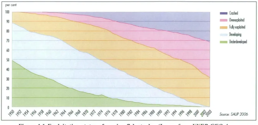
The main reasons for the decline in fish stocks (Figure 1.1) are a combination of unsustainable fishing, habitat degradation and global climate change. Declining fish stocks do not only cause loss of biodiversity, but they have serious implications for human well being too, with fish providing more than 2.6 billion people with at least 20 per cent of their average per capita animal protein intake (UNEP, 2007).
Source. SAUP 2006
per Lent 100
90
80
70
60
so
40
30
20
10
mom Crashed
[image:14.557.100.514.102.303.2]Overexploited Fut/ exploded Developing Underdeveloped
Figure 1.1 Exploitation status of marine fish stocks. (Image from UNEP GEO-4, 2007; source: Sea Around Us Project (SAUP) 2006.)
The ecosystem-based approach to natural resource management
is
a major principle underlying modern management practices (De la Mare, 2005; Garcia and Cochrane, 2005; Frid et al., 2006). It was adopted by the Parties of the 1992 Convention on Biological Diversity (CBD) as a strategy for the integrated management of land, water and living resources, that promotes conservation and sustainable use in an equitable way (Gjerde, 2006). A key element of ecosystem-based management is the establishment of Marine Protected Areas (MPAs). The CBD defines a marine protected area as "any defined area within or adjacent to the marine environment, together with its overlaying waters and associated flora, faunaand
historical and cultural features, which has been reserved by legislation or other effective means, including custom, with the effect that its marine and/or coastal biodiversity enjoys a higher level of protection than its surroundings."Scientific data mining for spatio-temporal hydroacoustic data sets
such as the North Atlantic, the Baltic Sea and the North Sea in the case of ICES, and the Southern Ocean and the Antarctic in the case of CCAMLR.
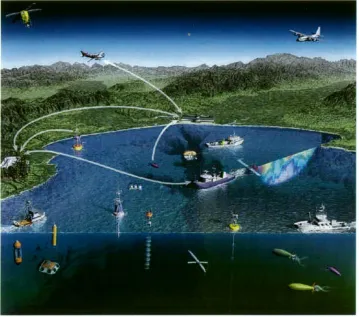
A wide range of sensing and measuring devices and instruments is deployed in the oceans, collecting very large amounts of scientific data. Measurements are made at varying spatial and temporal scales. These measurements lead to an understanding of the systems directly, or they can be used as input to mathematical models. Quantities of interest include ocean temperatures, currents, salinity and acidity levels, seabed depth and habitats. Observations of marine life are conducted by tracking tagged individuals or estimating abundance and spatial distributions of stocks. Instruments can be mounted on buoys, ships, or underwater vehicles. A graphic impression is given in Figure 1.2.
[image:15.565.84.443.363.680.2]Scientists from various disciplines are in need of tools, algorithms and systems to process and analyse these often disparate data sets, and to discover systematic patterns that can explain a system as complex as the global oceans. The work reported in this thesis represents a significant contribution to this field of research.
Figure 1.2 Depiction of a deployment of a multitude of sensors to observe the
1.3 PROBLEM DESCRIPTION
Acoustics is a common method used to study the underwater environment. Electromagnetic waves such as visible light are attenuated rapidly in water, whereas acoustic waves can propagate over long distances and penetrate to large depths. Acoustics is based on the examination of the characteristics of reflected sound (Urick, 1983). With respect to fisheries, acoustics is a more cost-effective and less intrusive method to conduct stock assessments than catching fish. Fisheries acoustics is the research area that studies the use of underwater sound to study fish, their behaviour, spatial distribution, and abundance (Simmonds and MacLennan, 2005).
Acoustic instruments for observing the aquatic environment are generally referred to as sonars. Echosounders, which are sonars with a single beam looking downward, are the standard acoustic devices used in routine fisheries surveys. Multibeam sonar systems have multiple beams pointing in different directions. Their use in fisheries research is relatively new. The use of multibeam sonar is well established for hydrographic applications, to measure the bathymetry or seabed depth. Sonar instruments designed for that purpose were typically not capable of collecting sound echoes from the water column, which is the body of water between the seabed and the transducer. However, most modern multibeam sonar systems designed for bathymetric applications can also collect data from the water column.
Multibeam sonars collect large amounts of data. Since the data are collected underwater using acoustic devices, the term hydroacoustic data is commonly used. Furthermore, the acoustic measurements are spatially and temporally referenced, hence the term spatio-temporal hydroacoustic data. Not only the data volumes but also the different instruments used to collect the data pose challenges in terms of data processing and analysis (Buelens et al., 2006). A recent ICES report refers to this problem as the data bottleneck (ICES, 2007b). A need exists to reduce this bottleneck: effective, fast, automated algorithms are needed to process and analyse the data into an intelligible, informative and manageable representation. This is the problem that is addressed in this research.
1.4 RESEARCH OBJECTIVES
Scientific data mining for spatio-temporal hydroacoustic data sets
A data mining process is a data handling and manipulation procedure leading to new insights in the data and what they represent (Cios et al., 1998). In fisheries research, these insights will contribute to improved biomass estimates and stock assessments, to a better insight in schooling behaviour, and generally a better understanding of ecosystems in which fish populations are an essential component. The data mining procedure is required to be able to handle the large amounts of data from various sonar instruments in a generic fashion. It must lead to an informative representation of the data in such a way that relevant higher level structures and concepts become available through the application of versatile and sophisticated algorithms.
1.5 THESIS SYNOPSIS
For this thesis, the two most important fields of research are underwater acoustics and data mining. General overviews of these subjects are given in chapter 2.
The data mining process that is presented in this thesis consists of two main phases: a data preprocessing phase and a pattern analysis phase, which are developed in chapters 3 and 4 respectively.
Chapter 5 contains case studies in which data are processed using the proposed data mining approach. Examples of modeled data, and real multibeam sonar and single beam echosounder data are given.
Many great advances in applied research occur when researchers from traditionally separate fields work together and combine their knowledge. One such area of research is fisheries acoustics. It has been a multidisciplinary field of research for decades. Contributors come from various disciplines including:
• physics (acoustics),
• engineering (instrumentation such as transducers),
• statistics, mathematics and computer science (data analysis), and • biology, ecology and oceanography (users of the systems and the data). Section 2.1 describes the field of underwater acoustics and the role multibeam sonar has started to play in recent years, particularly in fisheries research. Section 2.2 provides a general background on data mining and its role in the analysis of large data sets in general and spatio-temporal hydroacoustic data sets in particular.
2.1 UNDERWATER ACOUSTICS
2.1.1 Underwater acoustic measurements
Scientific data mining for spatio-temporal hydroacoustic data sets
such as size, age, or species exist and are a topic of ongoing research. Similarly, the determination of bottom characteristics is possible using acoustic techniques. General overviews of fisheries acoustics are given in Simmonds and MacLennan (2005) and Misund (1997). Determination of the bathymetry (seafloor depth) is commonly achieved using multibeam sonar (de Moustier, 1988; Hughes Clarke et al., 2000). A good overview of the state of the art in acoustic seabed characterization is presented in a recent ICES cooperative research report (ICES, 2007a). A general text on underwater acoustics is Urick (1983), and on acoustics Crocker (1998). This section is based on the references quoted, unless indicated otherwise.
Acoustics is the theory of sound propagating through a medium subject to scattering, reflection and absorption. Sound waves can propagate through water because of its elasticity which allows periodic compression and expansion. A sinusoidal sound wave is characterized by its frequency f, which is the number of cycles per second with which the pressure p varies relative to the ambient pressure level.
The sound speed c describes the speed with which wave fronts, or pressure peaks, move through the medium. The wavelength X is the distance between two consecutive peaks. The following relation holds:
c = f (2.1)
The sound speed is dependent on the medium. For water, c is typically in the range 1450-1550 m/s, depending on water temperature, ambient pressure and salinity. The wavelength poses a limit on the spatial resolution of targets when observed using acoustic instruments.
Sonar instruments transmit pulses comprised of a few cycles of a sine wave that lasts for a finite time: the pulse duration. Such a pulse is also referred to as a ping. Sonars commonly transmit pulses at frequencies centred in a narrow band around a centre frequency fo. This centre frequency is the frequency that is quoted when discussing sonar instruments. For most purposes the signals such systems generate are treated as single frequency signals. Wide band systems transmitting signals at a range of frequencies, or chirp systems which vary the frequency during transmission are not discussed in this thesis.
The pulse duration and the wavelength of the signal determine the resolution of a sonar in the along-beam direction. The across-beam resolution is dependent on the angular beam width and the range.
velocity v. In a plane wave, the pressure and particle velocity both vary as a sine wave and are in phase. The pressure, p, is related to the velocity, v, by the formula:
p= pcv (2.2)
where p is the water density. When a small source generates a wave, the wave fronts travel away from the source in all directions, in a spherical manner, and the wave is not planar. The relation between pressure and particle velocity is more complex in that case, and depends on the wavelength and the distance from the source. The far field of a source is determined by the distance at which the relation between pressure and particle velocity can be approximated by relation (2.2), a planar wave; the approximation does not apply in the so-called near field, or Fresnel zone.
A travelling wave carries energy. The flux J is the energy of the wave passing through a unit area perpendicular to the wave front. The intensity I is the energy flux per unit time. The intensity is the product of the pressure and the particle velocity:
I=pv=p 2 Ipc. (2.3)
Usually, the average intensity over one or more cycles of the wave is required, in which case the mean squared sound pressure is substituted for p. In particular, it is customary to work with root-mean-square (RMS) pressure amplitudes:
PR2MS = f(P(t) P0 )2 dt .
I cycle
(2.4)
In this thesis RMS pressure is assumed when using the term pressure or pressure amplitude.
The quantity:
Z = pc (2.5)
is the acoustic impedance, which is almost constant over the sound path in typical underwater environments.
Scientific data mining for spatio-temporal hydroacoustic data sets
Sonars transmit pulses by means of a transducer, which converts an electric signal
in an acoustic signal, thus generating a sound wave. Wave fronts travel outwards
from the transducer, spreading spherically. In the far field, the intensity
Ivaries with
the inverse square of the range
r:I = Io 1 r 2
(2.6)
where the range
ris the distance to the transducer, and
jo
is the reference intensity,
which is the intensity normalized to unit range.
Absorption is the loss of energy of a wave travelling through water. The lost energy
is converted to heat. This is due to the particle movements, with higher frequencies
incurring higher particle velocities. This is why low frequency waves penetrate
deeper into the water, as they lose energy less quickly. The pressure, and hence the
intensity of a wave decreases exponentially as:
= 10
10-
1
1°
(2.7)
with a the absorption coefficient.
When a wave is transmitted by a transducer, it travels away from it to encounter a
target such as a fish. A proportion of the energy of the incident wave is
backscattered by the target. This backscattered wave travels in the opposite
direction to that of the transmitted pulse, and is received some time later by the
transducer. In this thesis it is assumed that the same transducer is used for
transmission of a pulse and reception of its echo, or at least that the transducers are
close enough to be considered the same in practical applications.
The backscattering cross section
o-b,is a measure of the proportion of incident
energy that is backscattered by a target:
at. .r Ib i li2
(2.8)
with lb and
I,the backscattered and incident intensities respectively. The inverse
square law for energy spreading means that o
-
b, is a constant for a given target. The
target strength TS is the logarithm of the ratio of the backscattering cross section
and a reference area of 1 square meter (Clay and Medwin, 1977):
TS =
10 log
io
a
bs
(2.9)
For a target at a range r backscattering some of the incident energy, the time that elapses between the transmitted sound wave leaving the transducer and the backscattered signal arriving at the transducer is equal to the time needed for the sound wave to travel a distance of 2r. Hence, when an echo is received at the transducer at a time t after transmission, the range to the target responsible for that echo is:
r=ct12. (2.10)
A pulse of duration r, transmitted between times ti and t2, has a length in the range direction of:
ct2 / 2 — ct, / 2 = cy12 (2.11)
Since two targets can be resolved only when each of them results in a separate echo pulse, it is clear that targets that are closer than a distance of cr 1 2 cannot be observed individually.
In a situation when there are many targets close together, as is typically the case with fish schools, the targets form a combined return pulse, which does not allow for determination of individual targets of fish but which has an intensity that is still proportional to the combined target strengths of the individual scatterers (Foote,
1983). The volume backscattering coefficient s, is defined as: 1
sv
v iEv (2.12)
where V is the sampling volume and the sum is taken over all targets in V. The sampling volume is that volume for which targets within it are observable by the sonar. The logarithmic equivalent is commonly used, the volume backscattering strength Sv:
Sv =10 logio (2.13)
The importance of this theory is that it allows for the counting of the number of fish. When fish are not close together, the number of return pulses can simply be counted. In the other situation, considering eq. (2.12), and assuming that the distribution of the target strengths of the fish is known with expected value (crbs), eq. (2.12) can be written as:
n(ubs)
Scientific data mining for spatio-temporal hydroacoustic data sets
with n the number of targets in the volume V.
In situations where the transmitted sound pulse cannot penetrate to the deeper layers of dense fish schools, the shallower scatterers are said to cause a shadowing effect. This effect can lead to underestimation of fish numbers.
The value of s is directly calculated from the voltage output from a calibrated sonar (section 2.1.3). Based on knowledge of, or assumptions about, the target strength of the observed fish, eq. (2.14) can be used to determine their number, n. The underlying theory is that of echo integration, which is not elaborated on in this context. A good discussion, together with references to the original literature on the subject, can be found in section 5.4 of Simmonds and MacLennan (2005).
Until now the targets have been assumed to be point targets, or fish. Similar theory applies of course to scattering from the seafloor. However, a number of important differences exist. Unlike relatively small scatterers, the seabed is fixed in that it is not displaced by the incident wave. The way in which the incident energy is backscattered is different: the seabed can absorb much of the incident energy, or let the energy penetrate to certain depths from which it is backscattered slightly later than from the seabed surface. The references provided at the beginning of this section provide a good background on the subject. In the present context only two facts are relevant:
• the return pulse from the seabed can be used to determine the depth, or bathymetry,
• the characteristics of the return pulse can be used to derive properties of the seabed surface, such as its roughness or hardness.
2.1.2 Sonar instruments
It is instructive to differentiate between sonars that transmit and receive on a single channel using a mostly narrow beam, and sonars that transmit and receive on many channels simultaneously. The former are known as single beam sonars, the latter as multibeam sonars. General references on this subject include Mitson (1983) and Medwin and Clay (1998).
either stored directly or transmitted on a computer network, where they can be picked up by data logging software.
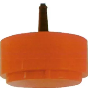
Single beam sonars and echosounders have circular or elliptical transducers (Figure 2.1). The size of the transducer determines the beam width of the acoustic beam, given the frequency. Beams are typically 5-15 degrees wide. All the elements in the transducer are activated simultaneously by the same electric signal, and the received signals are summed to constitute a single output signal. There are a number of variations that offer more possibilities; two common ones used in fisheries research are:
• Split beam echosounders allow for separate reception on each quadrant of a circular transducer. Using the phase differences between halves (pairs of quadrants), the direction of arrival of the received signal can be determined, through which it is possible to locate targets in the beam in three dimensions: range, as usual, and additionally two angular coordinates off the vertical.
[image:24.557.225.374.464.612.2]• Dual beam echosounders allow for separate transmission and reception on a circular subset of the circular transducer. The greater the diameter of the circle of activated elements, the narrower the beam. By using a wide and a narrow beam, the differences between the two signals can be used to determine how far off the central axis a target is located.
Figure 2.1 A 120 kHz transducer of a Simrad EK60 split beam echosounder.
Copyright: Simrad AS, Norway.
Scientific data mining for spatio-temporal hydroacoustic data sets
this is known as applying a time-varying-gain or TVG. TVG corrected signals are shown visually by means of an echogram: a visual display, with range on the vertical axis and the transmit times on the horizontal axis (Figure 2.2). Each sample is coloured by its backscatter amplitude, where warmer colours indicate higher amplitudes (what the actual values are is not relevant in the present context).
depth (m)
-3 - -38
-54 -58 -8 - 6 7
[image:25.564.175.349.536.681.2]transmit time (s)
Figure 2.2 Example of a single beam echogram from a Simrad EK500 echosounder (Sv values in dB).
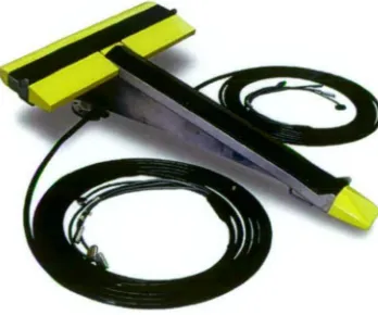
Multibeam sonars have transducers that consist of elements that are activated individually. The elements of such transducers are typically arranged in a linear flat or curved array. Since the beam width is very wide in the direction perpendicular to the direction of the array, it is customary to have one array for transmission, and another array perpendicular to the first for reception (Figure 2.3). This is known as a Mills-Cross array. Through this technique it is possible to attain narrow beams in both directions. The narrow beams are coplanar.
When transmitting, each element can be activated individually. This makes it possible to steer the beam electronically by changing the phase of the transmit pulse slightly from element to element. When this is done based on the input from a motion sensor, the beam can be stabilized for vessel motion such as pitch and roll. On reception, signals are received on the individual elements. The phases of these signals are used to form individual beams, pointing in different angular directions.
Until the early-to-mid 1990s, digital recording technology was not capable of outputting the complete signals for all elements. At the time, the signals were processed on dedicated Digital Signal Processing boards, which implemented algorithms to detect the bottom. The primary capability of such multibeam sonars was to get accurate bottom detections in each beam. The detections were output and stored to disk. Advances in technology have made it possible for complete multibeam sonar signals to be output, often together with the on-board determined bottom depths. The complete signal includes the backscatter returns from the water column.
The process of resolving the beams from the phase differences is known as beamforming, and is usually conducted prior to storing the data to disk, as is a TVG compensation. The backscatter amplitudes of the samples can be plotted in an echogram (Figure 2.4). All the data samples in such an echogram are collected from a single ping (one transmit-receive cycle). The corresponding single beam data are one vertical line of samples in Figure 2.2. In other words, a multibeam sonar collects a complete image as in Figure 2.4 for each vertical line of single beam data as in Figure 2.2.
depth
(m)
distance (m)
Scientific data mining for spatio-temporal hydroacoustic data sets
Typical multibeam systems collect data for 100-300 beams simultaneously. As a result, multibeam data sets are typically two orders of magnitude larger than single beam data files for the same number of pings.
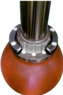
[image:27.565.206.318.247.414.2]Another class of sonars have cylindrical or spherical transducers (Figure 2.5). Their primary purpose is finding fish at long ranges from the vessel. As opposed to the two designs discussed above, this type of sonar has beams pointing typically in a circular fashion away from the transducer, forming a conical shape. To differentiate these models from the multibeam sonar described above, they are referred to as omnidirectional sonars.
Figure 2.5 Spherical transducer head of the Furuno FSV-30 series. Copyright: Furuno Electric Co. Ltd., Japan.
2.1.3 Multibeam sonar for water-column measurements
Multibeam sonar is the best and most widespread instrument to determine bathymetry, and at the same time bathymetry is the most common use of multibeam sonar (de Moustier, 1988; de Moustier and Matsumoto, 1993; Chakraborty and Schenke, 1995; Hammerstad, 1995; Mitchell, 1996; Pratson and Edwards, 1996; Brissette, 1997). Bathymetric multibeam sonar is an active field of research, for example the processing of bottom detections (Brouns et al., 2003; Calder, 2003; Canepa et al., 2003) or the inclusion of the backscatter amplitudes for the bottom detections, which provides insightful information of bottom types, characteristics and seabed habitats (Clarke et al., 1996; Keeton and Searle, 1996; Chakraborty et
The capability for multibeam sonars to output the complete signal, including the backscatter echo returns from the water column, rather than just that from the seabed, is recognized as having great potential for fisheries research. The main advantages over using echosounders were identified as increased sampling volume without loss of resolution, and extra spatial information. The first studies using multibeam water-column data concentrated on fish behaviour, such as vessel avoidance (Misund and Aglen, 1992; Soria et al., 1996), schooling behaviour (Gerlotto et al., 1999), predator-prey interactions (Noettestad and Axelsen, 1999) and fish migration (Hafsteinsson and Misund, 1995). Behavioural studies have continued since, providing new insights that would not have been possible to achieve without multibeam sonar (Axelsen et al., 2001; Johnson et al., 2001; Benoit-Bird and Au, 2003; Gerlotto and Paramo, 2003; Gerlotto et al., 2004; Brehmer etal., 2006; Gerlotto et al., 2006).
Behavioural studies are qualitative, in that the actual levels of the backscattered signals are not used to derive information about the observed organisms. In fisheries, an important aspect of surveys is estimating the number of fish, possibly specified to species or age group. When sonar is used for this purpose, it is said to be used in a quantitative manner. In order for quantitative work to be possible, a sonar has to be calibrated. Calibrating is the process of establishing values for parameters that are used in the calculation of target strength (TS) or volume backscattering strength (Sr) from the voltage signal from the sonar. One of the parameters in question is the on-axis sensitivity, which must be such that a target with a known target strength, placed in the centre of the acoustic beam, is observed by the sonar system to have that target strength. In a multibeam system, this has to be the case for each beam. The other parameter relates to the beam pattern of the acoustic beam, and is known as the equivalent beam angle, which is a measure of the beam width (Simmonds and MacLennan, 2005).
Scientific data mining for spatio-temporal hydroacoustic data sets
While water-column multibeam data have been used for more than a decade, there are a number of challenges that remain with respect to data processing and analysis (Buelens etal., 2006):
• The data volumes are very large. Since one ping of multibeam data contains two orders of magnitude more samples than its single beam equivalent, storing and handling multibeam data are an issue.
• Standardization is needed. Calibration is a good step towards ensuring that data are independent of the conditions under which they were collected. However, differences in instrumentation make it difficult to compare data collected with different instruments, including other multibeam sonar models, or even single beam and omnidirectional sonars.
• Visualization is important. The spatial complexity of multibeam data means that it is difficult to represent graphically, especially when data covering large areas or long time spans must be visualized simultaneously.
• Automation is essential. Since the data volumes are large and visual inspection is less straightforward than with single beam data, automated algorithms are needed to detect noise or errors in the data.
• Segmentation or object detection algorithms capable of identifying subsets of the data as coherent structures automatically is essential to aid in data analysis.
• Classification algorithms based on previously segmented data would be very useful to reduce processing and analysis time.
These are computational challenges, with solutions to be found in the field of computer science. The next section discusses computational aspects of data analysis.
2.2 DATA MINING AND PATTERN ANALYSIS
2.2.1 The data mining process
stored and accessed. Large data sets are being created and collected continuously, from sales and bank transaction records to seismic sensor recordings, from surveillance camera video footage to meteorological satellite imagery. Analysis of such data sets is often not trivial. Many data sets are very large, preventing human expert investigation. Classical statistical analysis can be of use, but is often limited because of strong assumptions that are needed, such as normality of distributions, or linearity of problems or models. These assumptions are not needed in many of the computational methods arising from computer science research (Breiman, 2001; Cox etal., 2001).
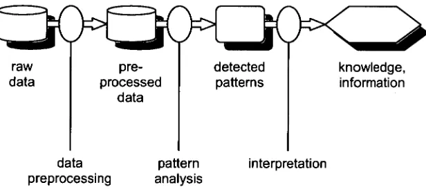
Data mining is the process of analysing data sets with the purpose of discovering previously unknown relationships or patterns. A number of introductory and review papers on the subject are available in the literature (Fayyad et al., 1996; Cios et al., 1998; Jain et al., 2000; Smyth, 2000; Grossman, 2001; Ramalcrishrian and Grama, 2001; Smyth, 2001; Ramalcrishnan, 2003; Yao, 2003). The data mining process can be presented as a stepwise process (Figure 2.6) (Van Hulle, 2004). When the data that are the subject of the data mining processes arise from scientific experiments, measurements or models, the term scientific data mining is used (Fayyad et al.,
1996; Grossman, 2001).
raw pre- detected knowledge,
data processed patterns information data
data pattern interpretation
[image:30.559.148.456.388.528.2]preprocessing analysis
Figure 2.6 Schematic overview of the data mining process.
Scientific data mining for spatio-temporal hydroacoustic data sets
Patterns arise when elementary data units are related in such a way that the relationship conveys information. Some examples are:
• Pixels constituting an image: individual pixels convey very little, but when combined as an image, they convey information about the subject in the image. The pattern is what is shown in the image.
• Sounds combined together to form words: the order and transitions of spoken sounds gives them the meaning of words and sentences. The sequential order of sounds constitutes patterns conveying information. • Credit card transaction data recorded by banks: individual transactions may
look legitimate, but when considered together with other transactions may indicate fraudulent card use. The patterns in transaction records can indicate legitimacy of card usage.
Before an algorithm is capable of identifying patterns in data, it must be tuned to do so. This tuning is commonly referred to as learning or training. In order to train an algorithm to perform a certain task, data are needed. In supervised learning, a data set is available and the patterns within it are known. In unsupervised learning, the patterns are unknown and must be discovered by the algorithm. In the examples above, data sets and their corresponding patterns are: images and what they show, sounds and what they mean, sets of transactions and whether they are legitimate or not. Pattern analysis algorithms aim to detect such patterns in new data that were not used in training the algorithm. This is an important aspect of such algorithms. they must generalize well to unseen data (Hastie etal., 2001).
The final phase of the data mining process consists of the interpretation of the detected patterns, which leads to new insights or information. This usually involves the graphical presentation of the raw or preprocessed data with an indication of the patterns. Where the data are spatial, as is the case in this research, it is customary to display the data in a spatial coordinate frame in two or three dimensions. Information visualization concerns the graphical representation of information, which is an important aspect of the final stage of the data mining process (Ware, 2004).
2.2.2 Spatio-temporal hydroacoustic data
stored and accessed. Large data sets are being created and collected continuously, from sales and bank transaction records to seismic sensor recordings, from surveillance camera video footage to meteorological satellite imagery. Analysis of such data sets is often not trivial. Many data sets are very large, preventing human expert investigation. Classical statistical analysis can be of use, but is often limited because of strong assumptions that are needed, such as normality of distributions, or linearity of problems or models. These assumptions are not needed in many of the computational methods arising from computer science research (Breiman, 2001; Cox etal., 2001).
Data mining is the process of analysing data sets with the purpose of discovering previously unknown relationships or patterns. A number of introductory and review papers on the subject are available in the literature (Fayyad et al., 1996; Cios et al.,
1998; Jain et al., 2000; Smyth, 2000; Grossman, 2001; Ramalcrishnan and Grama, 2001; Smyth, 2001; Ramakrishnan, 2003; Yao, 2003). The data mining process can be presented as a stepwise process (Figure 2.6) (Van Hulle, 2004). When the data that are the subject of the data mining processes arise from scientific experiments, measurements or models, the term scientific data mining is used (Fayyad et al.,
1996; Grossman, 2001).
raw data
pre- processed
data
detected patterns
knowledge, information
data pattern interpretation
preprocessing analysis
Figure 2.6 Schematic overview of the data mining process.
2 Background
georeferenced space, by means of its longitude, latitude and depth below the water surface. In addition, the time at which each sample is collected is available.
There are large differences between the size of data files collected by single beam instruments and multibeam instruments. Some indicative values are listed in Table 2.1. In practice data rates and file sizes can vary because of a number of factors, including the disk space needed for one sample (6 to 14 bits is common), the number of samples per beam (depends on the range and sampling rate), the ping rate (depends on range and vessel speed), and the size of the meta data and non-acoustic data such as position (these are small compared to non-acoustic data, and are not included in Table 2.1). Processing multibeam files containing data from a multi-day survey remains a challenge even with high-end computer hardware.
Single beam Multibeam
1
1201000 1000
10 pings/sec 2 pings/sec
1 KB 120 KB
600 KB/min 14.4 MB/min
864 MB 20.7 GB
Number of beams Samples / beam Ping rate
Ping size on disk Data rate / minute
File size 24 hours of data
Table 2.1. Some indicative values of data rates and file sizes, assuming one byte
per sample is needed.
Sonar manufacturers have not put substantial efforts in data compression, despite the fact that studies have indicated that suitable compression schemes exist, capable of compressing the data in a lossless manner to 70% of its original size (Wu
et al.,
1997; Pitman, 2002). Data thresholding and resampling seem to be the methods of choice to reduce the number of data samples. While thresholding is aimed at removing samples containing no information from scatterers, resampling is aimed at reducing the resolution and retaining some information from all samples. More advanced methods are conceivable, such as identifying noise and side lobing artefacts and removing the relevant samples selectively. Identifying redundancies in the data, such as those caused by repeated sampling of the same volume, and selective removal of the relevant samples is another alternative. More research is needed for these advanced methods to become common practice; the methods developed in chapter 3 of this thesis deliver a contribution in this area.intervention, are not suitable for large data sets, or are often not general enough to be applicable to data collected by different instruments. The methods developed in chapter 4 of this thesis offer an alternative approach.
Another important aspect that has not received much attention is that of standardization of multibeam water-column data, for easy sharing, storing and using of the data sets. There are a number of initiatives that are relevant in this context. The ICES Working Group for Fisheries Acoustics Science and Technology (WGFAST) have edited and adopted a standard data format for fisheries acoustics raw and edited data: HydroACoustic data format (HAC) (ICES, 2005). HAC is designed for single beam echosounder data, including dual and split beam, but does not currently cover multibeam data. It is unclear at this stage whether the format will be extended in the future.
For data sets to be exchangeable and distributable, good metadata is vital. Metadata is the description of the actual measurement data, such as names, units, scales, and descriptions. If data is to be shared at a global scale, global initiatives are needed. One such example is the Marine Metadata Interoperability project (MMI), established to promote the exchange, integration and use of marine data through enhanced data publishing, discovery, documentation and accessibility (MMI, 2007). Hundreds of institutes and organizations world wide are making their marine and oceanographic data available through data centres or repositories. It is essential that data can be shared across data centres, which is facilitated by using the same data formats and metadata definitions. The Intergovernmental Oceanographic Commission (IOC) of UNESCO has been running its International Oceanographic Data and Information Exchange (IODE) facility since 1962 to enhance marine research, exploitation and development by facilitating the exchange of oceanographic data and information between participating member states and by meeting the needs of users for data and information products (IODE, 2007).
ICES has a working group on marine data management. The activities of this group include the establishment of guidelines with respect to data and metadata storage and access (ICES, 2006). It can be expected that formulated advice will be in line with the corresponding IODE guidelines.
3 DATA PREPROCESSING
3.1 OBJECTIVES
Modern computer hardware is capable of storing the large amounts of data collected by multibeam sonars on hard disks. However, hard disk access is still relatively slow, and data processing can be computationally intensive, particularly for some advanced and complex algorithms. It is therefore desirable to reduce the data volume while retaining as much information as possible. A second and equally important aspect is normalization across instruments and instrument settings. From the point of view of postprocessing analysis algorithms it is desirable to have the acoustic measurements in a unified form and format, from which any instrument-specific details are removed.
3.2 ACOUSTIC MODELING
3.2.1 Concept
Given an underwater environment including aggregations of fish and the seabed, what would this look like when observed with a multibeam sonar instrument? In this section a forward model is developed that answers this question. The ultimate question is the reverse: given the data recorded by a multibeam sonar instrument, what did the underwater environment consist of in terms of scatterers such as fish schools and the seabed? In order to answer the latter question, the forward model must be inverted. This is discussed in the next section.
Besides the primary goal of establishing an analytical description of the process that must be inverted, a secondary benefit of a forward model is that it enables the creation of arbitrarily simple or complex data sets. This will prove very useful when evaluating inverse models, due to the difficulty of obtaining real-world ground truthed data sets.
The forward model incorporates two components: an acoustic model, in this case an acoustic ray tracing model, and a model of a multibeam sonar. The input to the model consists of a description of a three-dimensional underwater scene in which the multibeam sonar will be deployed. The output consists of a sequence of complex-valued sonar data sets, commonly referred to as pings. A schematic overview is shown in Figure 3.1.
Model of aquatic environment
Model
Acoustic ray tracing model
Multibeam sonar model
Acoustic multibeam data
Figure 3.1 Overview of the forward model, its two components and its input and
3 Data preprocessing
3.2.2 Model input
The input to the acoustic model is a model of the aquatic environment consisting of a description of a three-dimensional underwater scene, containing a seafloor surface and volumetric objects representing aggregations of fish. It is assumed that the multibeam sonar is mounted on a vessel surveying the area of the three-dimensional scene. A trajectory for that imaginary vessel can be defined. In its simplest form, it is assumed that the acoustical characteristics of the seabed (hardness and roughness) are constant for the whole surface. Furthermore, it is assumed that the distribution of the number of fish in the fish schools is Poisson. The Poisson distribution is given by:
( n ) = Vie'
n! (3.1)
where v is the Poisson parameter, which in this case is equal to the average distance between individuals in the aggregation. The quantity P„ (n) gives the probability of n individuals occurring in a unit volume within the school.
The acoustical properties of the seabed and the density of fish within a school is parameterized, as well as the target strength of the fish in the school. Both the seabed and the fish schools are modeled by individual point scatterers (Middleton, 1967; Olishevskii, 1967; Bell, 1997; Tillett et al., 2000). In the case of the seabed, the scatterers are placed close enough to each other for the model to treat it as a solid surface. The density of such points on the seabed surface depends on the frequency of the sonar, and is such that the mean distance between two points is less than a quarter of the wavelength of the sonar system. Fish schools are modeled as point targets in an enclosing volume shell. The target strength of the point scatterers is the average target strength of the fish species being modeled.
The point model is defined as
=
fp,}
with 0 i N,... 0 ... .0 ... 0 ...
—0 ...
0 ... 0 ...
44 i2dor,
Awl '-'
Figure 3.2 The black dots represent the pi in SI . The dotted line is the vessel cruise track; the white dots represent the locations where a multibeam ping will
occur.
3.2.3 Acoustic ray tracing
Different standard acoustic computational models are described in the literature, including Urick (1983) and Crocker (1998). For the purpose of modeling multibeam sonar, acoustic ray tracing offers a computationally feasible and straightforward yet sufficiently sophisticated approach (Ziomek, 1989; Bell, 1997; Bell and Linnett, 1997; Etter, 2001). The ray tracing model computes the acoustic pressure at each element of the transducer face. Each pressure value is obtained by combining the responses of the scatterers in the point model. The following equation describes the ray tracing model:
p 1(t) = Egi,kPOAkWt(tk+ tk,j)1°-2ar(k)/10 r(0-4 + g
o,
j, (3.2)k=1
with:
p (t) the pressure received at time t in ping i by transducer element
gi,k= 1 if point k is in the transmit beam for ping i, gi,k= 0
otherwise,
PO the reference pressure level (transmit pressure as measured at
lm from the transducer),
3 Data preprocessing
Ak = abs(k) r(k)
10-2ar(k)/10 r(0-4
11(i, ,t)
with r(k) the distance from the array centre to point k, and Crbs(k) the backscattering cross section of point k,
absorption and spreading loss, with r(k) as above and a the absorption coefficient,
an additive noise term, which in the model can be set to Gaussian, or zero,
W, (tk + ) the eikonal at time t, evaluated at time tk + , where tk is the acoustic travel time from the centre of the transmit array to point target k, and tc., is the travel time from point target k to element j of the receive array. W is a function of the
transmitted pulse shape and pulse length:
(s) = tc(t — s) where K(.) is the transmit pulse. For example, with KO a block pulse, K(t) = el" for 0 < t < T, and 0 otherwise; T is the
pulse length and co is the angular frequency, co = 2af, with f the operating frequency of the multibeam sonar.
Calculation of tk and tk + tk,., requires knowledge of the sound speed c (provided as a parameter), and of the geometry of the multibeam transducer. Knowledge of the transducer arrays is assumed. Only first order scattering is considered as this is known to be the dominant effect (Foote, 1983).
3.2.4 Modeling multibeam sonar
A parameterized model of a generic, typical multibeam sonar is developed. The receiving transducer array is assumed to be a flat linear array. Its length and the number of individual transducer elements are parameterized, as well as its operating frequency. Known and published recommendations for transducer element sizes are adhered to: the element spacing I must be chosen such that I212, for a wavelength 2 in order to avoid spatial aliasing (Knight etal., 1981).
The acoustic ray tracing model, eq. (3.2), allows for calculation of the pressure
levels at each of the transducer array elements, as a function of time. The multibeam
transducer model will 'measure' these pressures
p,,,(t)as voltages
V,,, (t)for ping
i,element
j, at time t.A sampling rate can be chosen, and the voltages are digitally
sampled accordingly. A time varied gain (TVG) is applied to the voltages to
compensate for the absorption and spreading losses. TVG-compensated samples are
written to disk by the model, and are referred to as the raw data. Discrete complex
raw data samples are denoted by c
id
,„ where
iand j are as before, and
sis the
sample index for increasing ranges, 0... S-1 for
Ssamples. With f
sthe sampling
frequency of the system, c
j
,j,= P1,J
(s /j).The raw data is subsequently beamformed. The beam former implemented in the
model is the standard Fourier-based beam former (Rudnick, 1969). A beamformed
complex data sample in ping
i,beam], range index s is obtained as:
d1 5 w(j, s, k ,1)e
(3.3)
where the summation over
k is over the transducer elements and over / is over therange indices of the samples, and:
0k,j = dk
sin(a)/2
(3.4)
where 2 is the wavelength of the acoustic signal,
dk is the distance from the centre ofthe array to the centre of transducer element
k and c tis the angle of the central axis
of beam
].The function
w(j, s, k, 1)is a windowing function. Different choices are possible, all
with specific advantages and trade-offs, see for example (Curtis, 1998; Chu
et al.,2001b). Windowing functions not being the focus in this context, a simple
windowing function is chosen:
w(j, s, k, I) =
1 if / = s,
for all k and
j,w(j,
s, k, 1) = 0 otherwise.With this choice for w, equation (3.3) reduces to:
d 1 Ci,k,s
(3.5)
3 Data preprocessing
(squared amplitude), which is often the only information that is written to disk by real-world multibeam systems, aid, =
3.2.5 Model output
Some formalism is introduced. The set of points is the input to the model, resulting in the beamformed data samples d,,j,s. Defining A = clus ) and denoting the analytical model with M, the modeling process is written as:
(3.6) The data generated by the model is referred to as synthetic data. Acoustic data are commonly represented graphically as an echogram: a colour-coded image of the signal amplitudes. An example of an echogram of beamformed synthetic data is given in Figure 3.3. This example is from the data file that is discussed in detail as a case study in section 5.1.
.1
-1-18 -2
-47 -5 -58 -64 -7
Figure 3.3 Echogram representing one ping of synthetic data, showing two
aggregations of fish above a flat seabed (Sv in dB).
3.2.6 Model validation
Statistical validation
The simplest form of model validation is determining whether the synthetically generated acoustic data resemble true acoustic data. When represented as echograms, the human eye perceives the synthetic data as plausible, but an objective statistical measurement of similarity to real data must be made in order to substantiate such a claim. A criterion for similarity can be stated as (Bell and Linnett, 1997):
Definition 3.1 (Statistical similarity). Two acoustic data sets are defined to be statistically similar if their constituting amplitude values are likely to be drawn from the same probability distribution.
Theoretically, it is expected that the Probability Density Function (PDF) of full water-column multibeam amplitude data values follows the K-distribution (Di Bisceglie et al., 1999; Chitroub et al., 2002; Abraham and Lyons, 2004). The K-distribution is well established as a model for the amplitude statistics of scattered waves (Jakeman and Tough, 1987; Hongler, 1988; Jakeman and Tough, 1988; Lyons and Abraham, 1999), and is given by:
4 v )1/2 v 1/2 v 1/2 PK (x) = F(v) ,u p — x K — x
where
ro
is the gamma function, Ky., is a modified Bessel function of the second kind, of order v-1, and v and ft are the parameters of the distribution. The parameter p is the mean, and v is the order parameter. The order parameter can be interpretedas the amount of coherent clutter in the data (Abraham and Lyons, 2002); coherent clutter arises when there are non-random aggregations of scatterers causing coherence in the echo return signal.
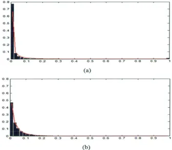
Given a data set, the parameters are estimated using the standard Maximum Likelihood (ML) method (Pesavento et al., 1998). Whether the amplitudes of a given data set are K-distributed is assessed using the Pearson x2-test, with the null hypothesis Ho: 'The distribution of the amplitude values follows a K-distribution'. First, a selection of multibeam pings from data sets collected by real instruments is tested, including data from a Simrad Mesotech SM2000 sonar (Figure 3.4 (a)). Structural noise must be avoided, since that can distort the amplitude sample distribution. Structural noise can be caused for example by interference with other acoustic instrumentation on board the vessel. The null hypothesis can not be rejected at the 5%-significance level on the basis of the data considered (p= 0.0346 <0.05). Second, a selection of pings from the synthetic data set shown in Fig 3.3 and discussed in section 5.1 is tested (Figure 3.4 (b)) This again does not lead to a rejection of the null hypothesis at the 5%-significance level (p= 0.0165 <0.05).
3 Data preprocessing
In Figure 3.4, histograms of real and synthetic data are shown, with the K-distribution PDF (3) overlaid, using the ML-estimates of the parameters and v and p. This statistical assessment shows that the synthetic data obtained through the model are similar to real data, according to definition 3.1. The target strength and spatial distribution of the scatterers do affect the parameters of the distribution, but do not affect the nature of it: amplitude values are K-distributed under sometimes very different scattering regimes.
0.8
0.1
06
05
04
0.3
02
01
O
o 01 02 0.3 04 05 06 07 08 09 1
(a)
[image:43.562.128.464.216.510.2](b)
Figure 3.4 Histograms (bars) and ML estimates of the K-distribution PDF (lines)
for (a) real data and (b) synthetic data. The synthetic data had more scatterers in
the water column than the real data, explaining the more gradual drop-off in (b). The artefact in the bin at the value of 1.0 in (a) is due to the limited dynamic
range of the instrument used (SM2000), causing saturation of the echo signal.
Simulation of a real-world data collection scenario
Definition 3.2 (Validity). The multibeam data collection model is valid if the resulting synthetic data resemble real data resulting from monitoring a real environment with a real multibeam sonar. The input to the model must be an accurate description of the real underwater scene.
This latter condition prevents thorough testing for validity, because, typically, an exact description of the underwater environment is not available. Further issues are that the actual multibeam sonar instrument used is likely to have peculiarities causing it to differ from the modeled system, that random noise in the real system affects the outcome, and that some simplifications and assumptions have been made in the model.
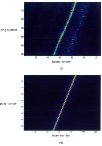
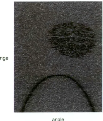
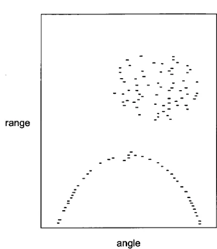
The only real-world multibeam data sets that are collected under controlled circumstances in a known environment are taken in test tanks, most commonly during calibration experiments. Such a data set was obtained (courtesy of Dr K. Foote and Dr D. Chu at Woods Hole Oceanographic Institution, USA). This data set contains full water-column data collected in a dock, in a controlled calibration experiment, with a Kongsberg Mesotech SM2000 multibeam system. A calibration sphere was moved through the beams in steps of 0.2 degrees, and kept at a constant range of 11 meters. A description of this scenario is assembled, and used as input to the simulation model. The resulting synthetically generated data set is studied in comparison with the real data set. A calibration is performed on both the real and the synthetic data sets (Cochrane et aL, 2003; Foote et al., 2005), and the resulting calibrated sets are subsequently compared. At each angular position of the sphere, all the samples at a range of 11 meters are selected and stacked up to form a single image, representing a sweep of the calibration sphere through the beams. This is done both with the real data as well as with the synthetic data, and the resulting images are shown in Figure 3.5.
Unfortunately in Figure 3.5 (a), the ping rate and the movement of the sphere were not synchronised, resulting in an unequal number of pings per sphere position, explaining the slightly curved nature of the sphere trajectory as observed in Figure 3.5 (a).