Adaptive Fault-Tolerant Control of Spacecraft
Attitude Dynamics with Actuator Failures
Yu Han1
Harbin Institude of Technology, Harbin, Heilongjiang, China, 150001
James D. Biggs2
University of Strathclyde, Glasgow, G1 1XJ, UK
Naigang Cui3
Harbin Institude of Technology, Harbin, China, 150001
Nomenclature
¯
A = the local vertical and local horizontal reference frame ¯
B = the body-xed reference frame
J = inertia matrix of spacecraft
ω = angular velocity vector of spacecraft (rad/s)
¯
q, q, q4 = quaternion of spacecraft
τ = control torque input vector of spacecraft (Nm)
ˆ
ω = angular velocity vector of ideal reference model (rad/s)
ˆ ¯
q,q,ˆ qˆ4 = quaternion of ideal reference model
ˆ
τ = control input vector of ideal reference model (Nm)
¯
θ = adaptive parameter of angular velocity
¯
δ = adaptive parameter of quaternion
Fg = the gain matrix
1 Ph.D. candidate, School of Astronautics, Mailbox 345, Harbin Institude of Technology, Harbin, China, 150001, [email protected]
2 Associate Director, Advanced Space Concepts Laboratory, Department of Mechanical and Aerospace Engineering, University of Strathclyde, Glasgow, G1 1XJ, UK, [email protected]
gi = actuator gain fault indicator for theith actuator
Fd = the deviation matrix
di = actuator deviation fault indicator for theith actuator
R(¯q)= rotation matrix
I. Introduction
Spacecraft play an increasingly important role in various areas of modern society, such as
telecommunication, earth observation, and space exploration. It is estimated that there have been
more than 7000 spacecrafts launched all over the world. Despite rigorous testing many of these
spacecraft fail on orbit due to various reasons [1], which consequently often lead to the failure of
the whole mission. According to [2], over 30% of spacecraft failures occur at the subsystem level
of the Attitude and Orbit Control System (AOCS). Moreover about 50% of the AOCS failures are
attributed to actuator errors. The purpose of this paper is to present an actuator fault-tolerant
attitude control.
In this paper, we distinguish between three types of actuator error, which are consistent with
the faults that can occur in reaction wheels [3]: (i) A gain fault [4], which represents a case in
which one or several actuators lose partial power but still function; (ii) A deviation fault, where
an actuator delivers a constant torque in addition to the required torque; (iii) A stuck fault, which
means the actuator output is stuck at a constant value of torque despite a dierent required torque.
Previous work in the literature on fault-tolerant control focuses on just one type of fault mode,
[46]. This paper considers a control method which could work in the presence of all of these faults.
In this paper we look at applying an adaptive control to the attitude control of a spacecraft in the
presence of these actuator faults. Adaptive control refers to a control that adapts to accommodate
parametric, structural, and environmental uncertainties to achieve a desired system performance,
[7]. Such uncertainties often appear in aerospace actuators and automobile engines, electronic
devices, and industrial processes. Payload variations or component wear and tear or even complete
failure of components lead to parametric and structural uncertainties in the modelling; in addition
leads us to consider a stochastic element in the modelling and a control must adapt to deal with
such unknown quantities. Adaptive control has been developed in both theory and application to
challenging problems of robustly controlling uncertain systems. Unlike the classical controllers, such
as PID, which are conventionally based on the assumption of known system parameters, adaptive
controllers do not have this strict requirement; they can adapt to parameter uncertainties by using
performance error information on-line.
Conventional attitude controllers such as quaternion feedback control are tuned assuming that
the system works perfectly where the parameters and constraints of the system are known [8, 9].
However, they do not take into account the re-tuning required in the event of an actuator fault. In
this paper, we use an ideal reference model to identify an actuator fault where a fault is identied
when the real system deviates from the ideal model. The control tracks the controlled ideal reference
model to replicate it as closely as possible. Two adaptive parameters are used which increase the
responsiveness of the tracking control to deviations from the ideal reference state. Moreover, it is
shown that the angular velocity relative errors are more sensitive than quaternion relative errors to
actuator faults. Thus the adaptive parameter shifts the emphasis to tracking the angular velocity
error more aggressively than the quaternion error in the presence of a fault.
In the following section we describe the attitude kinematics and dynamics of the spacecraft and
ideal reference model. Section III then addresses the problem of developing an adaptive controller
in the presence of uncertainties and actuator failures. Section IV illustrates the applicability of
the adaptive control through the simulation of a nano-spacecraft. Through comparing the adaptive
control of this paper to a conventional proportional controller, we can see the adaptive control
demonstrates an improved control performance.
II. Spacecraft System Model and Ideal Reference Model
In this paper, the dynamics of the spacecraft system can be modeled as a rigid body with
negligible moving parts and no liquid propellant. In contrast to classical proportional controllers
that track a reference trajectory or desired steady state, this spacecraft controller tracks the state of
for the attitude kinematics and dynamics of the spacecraft and the ideal reference model.
The spacecraft system is considered as a rigid body. The local vertical and local horizontal
(LVLH) reference frame A¯ with its origin at the centre of mass of an orbiting spacecraft has a set
of unit vectors{~a1, ~a2, ~a3}, with~a1 along the orbit direction,~a2 perpendicular to the orbit plane,
and~a3 dened by the right-hand rule, towards the Earth, [9]. Dene also a body-xed reference
frameB¯ with basis vectors{~b1,~b2,~b3}. The spacecraft attitude is then dened as the relative angle
from the local-level coordinates to the body frame. Dene ω×,ω = [ω1, ω2, ω3]T, by the following
skew-symmetric matrix:
ω×≡
0 −ω3 ω2
ω3 0 −ω1
−ω2 ω1 0
(1)
The Euler equations of motion describing the spacecraft motion in the body-xed reference frame
can then be expressed as [9, 10]:
Jω˙ =−ω×J ω+τ (2)
where J ∈ R3×3 denotes the positive denite, symmetric inertia tensor of the spacecraft; ω =
[ω1, ω2, ω3]T denotes the angular velocity vector of the spacecraft model with respect to the local reference frameA¯ and expressed in the body-xed frameB¯; andτ = [τ1, τ2, τ3]T denotes the control
torque input vector.
The attitude kinematics of the spacecraft is parameterised using quaternions:
2 ˙q=q4ω−ω×q (3)
2 ˙q4=−ωTq (4)
where q¯ = (q, q4) ∈ R3×R with q = [q1, q2, q3]T denotes the unit quaternion representing the
attitude orientation of the ideal model in the body-xed frameB¯ with respect to the inertial frame
¯
A, which are subject to the constraint
ω× is an element of the Lie algebra of the rotation group SO(3) whose Lie bracket is dened by
[X, Y] =XY −Y X. The Lie algebraso(3)is isomorphic toR3[11]. A rotation matrix can then be
retrieved fromq¯as:
R(¯q) = (q42−qTq)I3×3+ 2qqT −2q4q× (6)
whereI3×3 is a3×3 identity matrix.
In this paper, an idealized system under normal operating condition is set. If the adaptive
control logic detects any dierence between the ideal model of the system state under control and
the actual state of the system, a fault is identied. The angular velocity of the ideal reference
system is ωˆ = [ˆω1,ωˆ2,ωˆ3]T. The unit quaternion of the ideal reference system is qˆ¯= [ˆq,qˆ4] with
ˆ
q= [ˆq1,qˆ2,qˆ3]T and the control torque of the ideal reference system isτˆ= [ˆτ1,τˆ2,τˆ3]
The dynamic and kinematics of the ideal reference model is:
Jω˙ˆ=−ωˆ×Jωˆ+ ˆτ (7)
2 ˙ˆq= ˆq4ωˆ−ωˆ×qˆ (8)
2 ˙ˆq4=−ωˆTqˆ (9)
which can be in rotation matrix form as R˙(ˆq¯) =R(ˆq¯)ˆω×
In the actual spacecraft system, the control objective is to track the ideal model with the angular
velocity vectorωˆ and the quaternionqˆ¯. The quaternion error is thus dened as
eq1
eq2
eq3
eq4 = ˆ
q4 q3ˆ −q2ˆ −q1ˆ
−qˆ3 qˆ4 qˆ1 −qˆ2
ˆ
q2 −qˆ1 qˆ4 −qˆ3
ˆ
q1 q2ˆ q3ˆ q4ˆ q1 q2 q3 q4 (10)
where e¯q = [eq, eq4]T andeq = [eq1, eq2, eq3]T denotes the quaternion error, which is equivalent to
R(¯eq) =R(ˆq¯)TR(¯q)then
˙
which simplifys to
˙
R(¯eq) =R(¯eq)(ω×−R(¯eq)−1ωˆ×R(¯eq)) (12)
Dening the relative velocity ase×ω =ω×−R(¯eq)−1ωˆ×R(¯eq), the equation (12) comes to R˙(¯eq) =
R(¯eq)e×ω which can be expressed in quaternion form as
2 ˙eq=eq4eω−e×ωeq2 ˙eq4=−eTωeq (13)
whereeω=ω−R(¯eq)Tωˆ.
III. Adaptive Fault-Tolerant Control Logic
In this section an adaptive fault-tolerant control logic is presented which is robust to actuator
faults. The actuator gain fault and deviation fault is considered. This section presents an adaptive
fault-tolerant control logic that incorporates actuator faults and uncertainties.
A. Adaptive Control Logic and Stability Proof
The adaptive control logic of the actual spacecraft system is stated as
τ=ω×J ω−Ωˆ −θe¯ ω−δe¯ q4eq (14)
whereΩ =ˆ J e×
ωR(¯eq)Tωˆ+J R(¯eq)TJ−1(ˆω×Jωˆ−τˆ).
This paper shows that this controller is robust to certain faults through mathematical proof and
numerical simulation. However, before proceeding to address the stability properties and simulation
we provide some intuition into the choice of denitions of the adaptive parametersθ¯and¯δ.
˙¯
θ=kθ< eω, eω>R3 (15)
˙¯
δ=−kδ < eq, eq >R3 (16)
where kθ > 0 and kδ ≥ 0. The adaptive parameters θ¯ and ¯δ are positive and are written as
¯
Theorem 1 Let eωd = [0,0,0]T, eqd = [0,0,0,1]T be the desired attitude of the system. For
any tracking error(eω, eq)of the spacecraft system without actuator faults (2) with the control (14).
Then the tracking erroreω→eωd, eq→eqd ast→ ∞.
Proof: Dene a general Lyapunov function as
V ≡ 1
2 < J eω, eω>R3 +¯δ < eq, eq >R3+ 1 2kθ
( Z
˙¯
θdt)2 (17)
The time derivative of this Lyapunov function is given by:
˙
V =< J eω,ω˙ −R˙(¯eq)Tωˆ−R(¯eq)Tω >˙ˆ R3 +2¯δ < eq,e˙q >R3 + ˙¯δ < eq, eq >R3 + 1
kθ (
Z ˙¯
θdt) ˙¯θ (18)
then substituting equation (2), (7),(15) and (16) into equation (18) gives:
˙
V = < eω,−ω×J ω+τ+J e×ωR(¯eq)Tωˆ+J R(¯eq)TJ−1(ˆω×Jωˆ−τˆ)>R3 +¯δ < eq, eq4eω−
e×ωeq >R3 −kδ < eq, eq >2R3 +( Z
˙¯
θdt)< eω, eω>R3
(19)
takeΩ =ˆ J e×
ωR(¯eq)Tωˆ+J R(¯eq)TJ−1(ˆω×Jωˆ−ˆτ), and since< eq,−e×ωeq >R3= 0, the equation (19) simplies to
˙
V =< eω,−ω×J ω+τ+ ˆΩ + ¯δeq4eq+ ( Z
˙¯
θdt)eω>R3 −kδ < eq, eq >2R3 (20)
setting the control law to equation (14) gives:
˙
V =−θ¯(0)< eω, eω>R3 −kδ < eq, eq>2R3≤0 (21)
Thus, the result as stated in Theorem 1 is established.
B. Actuator Fault Modes
Two main kinds of actuator fault for spacecraft are a gain fault and a deviation fault. The
actuator fault changes the control torque of the spacecraft model, which is dened by:
τ=Fgu+Fd (22)
where u = [u1, u2, u3]T denotes the desired control torque, Fg ∈ R3×3 is the gain fault matrix
fault. So for the adaptive control logic (14). The gain matrix is expressed as [4],
Fg=
g1 0 0
0 g2 0
0 0 g3
(23)
the gain fault indicator 0≤gi≤1can be continuous time-varying or stochastic where a stochastic
element would represent uncertainty in the actuator fault. The case in which gi = 1 implies that
the actuator is not in a gain fault mode;gi = 0 is the case in which the ith actuator is in a stuck
fault mode; and0< gi<1 corresponds to the case in which theith actuator partially loses power
(gain fault mode).
For the deviation fault matrix,di is the deviation fault indicator for theith thruster, which
is also uncertain. The case in whichdi = 0 implies that the ith actuator is not in deviation fault
mode.
It has been shown that an increase in the gain matrix related to the angular velocity error
greatly improves the control performance in the presence of an actuator fault [12]. When there is
an actuator fault, the gain on the angular velocity error will increase to compensate for the increase
in error. However, when the actuators are operating close to their maximum torque, the increase
in the gain parameter could push the desired torque beyond the physical capability of the actuator.
Therefore, to oset this increase in torque the gain related to the quaternion error could be reduced.
This approach, therefore, places a greater weight on tracking the reference angular velocity relative
to the reference quaternion in the presence of an actuator fault. The control presented in this paper
is based on this reasoning and is also shown to guarantee asymptotic stability in the presence of a
gain and stuck fault using a Lyapunov function later in the paper. This approach is informed by
the observation that the angular velocity relative error is more sensitive to actuator faults than the
quaternion relative error. To illustrate this point we simulate two identical spacecraft to perform a
typical slew maneuver using a quaternion feedback controller of the form [9]. The rst spacecraft
considered (Spacecraft 1) is assumed to experience no faults and we dene its angular velocity as
ωo and its quaternion asqo. A second spacecraft (Spacecraft 2) is considered to have a gain fault
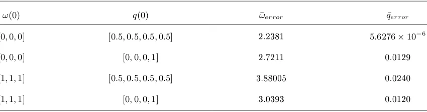
Table 1 The impact of actuator fault to relative errors
ω(0) q(0) ω¯error q¯error
[0,0,0] [0.5,0.5,0.5,0.5] 2.2381 5.6276×10⁻⁶
[0,0,0] [0,0,0,1] 2.7211 0.0129
[1,1,1] [0.5,0.5,0.5,0.5] 3.88005 0.0240
[1,1,1] [0,0,0,1] 3.0393 0.0120
Spacecraft 2 is denoted asωf and its quaternion byqf
gi= 0.3 + 0.1rand(t) + 0.2sin(500t+iπ/3) (24)
d1= 0.00001 (25)
We dene the relative error of angular velocity as
ωerror=
kωf−ωok kωf k
(26)
and the relative error of the quaternion as
qerror=
kqf−qok
kqf k (27)
Table.1 shows the arithmetic mean of the relative error of angular velocity and the quaternion
for a few examples of dierent initial conditions of the spacecraft motion. It shows clearly that the
arithmetic mean value of the relative error of angular velocityω¯error is much larger than the
arith-metic mean value of the relative error of quaternionq¯error in all the situations that are considered.
Therefore, it is intuitive to increase the gain on the angular velocity error relative to the quaternion
error due to the greater eect of a fault on the relative error of the angular velocity as shown in the
control logic (14), (15), (16).
IV. Simulation Study
The following section is used to verify the eectiveness of the proposed control scheme. We
dimensions10×10×10cm, with the moments of inertia
J =
0.0109 0 0
0 0.0506 0
0 0 0.0509
This type of nano-spacecraft does not undergo the rigorous testing of a conventional multi-tonne
spacecraft and thus is more susceptible to faults. The real UKube-1 is not equipped with reaction
wheels; nevertheless, this type of actuator (3-axis stabilization) is used in the simulations. In this
paper we use large magnitudes for the actuator faults as it enables the demonstration of the control
to be illustrated most eectively. However, using these large magnitudes for the faults means that
the corresponding desired torque is out-with the current nano-spacecraft reaction wheel capability.
In this paper, a simple quaternion feedback controller [14] can be used to perform a simple slew
maneuver for the ideal system:
ˆ
τ=−σJωˆ−kJqˆe (28)
where σ, k >0 are scalar constants, which can be extended to counter the unwinding problem by
introducing a discontinuity. The quaternion error of the reference model qˆ¯e = [ˆq1e,qˆ2e,qˆ3e,qˆ4e]T
is calculated from the commanded attitude quaternion qˆ¯c = [ˆq1c,qˆ2c,qˆ3c,qˆ4c]T and the current
quaternionqˆ¯as equation (10). In this paper, the simulation is taken with a simple baseline maneuver
which is planned rest-to-rest from qˆc(0) = [0,0,0,1]T to qˆc(Tf) = [0.5,0.5,0.5,0.5]T. The initial
value of the adaptive parameters in the control logic (14) can be chosen as the parameters in the
ideal reference model (28) such that θ¯(0) =σandδ¯(0) =k.
A. Simulation with a Gain Fault
In general this fault can be expressed in the formgi =α+βrand(t) +sin(γt+iπ/3) withα
as a mean value; rand(t)a random number between 0 and 1, and sin(γt+iπ/3) is time-varying.
This general form can be used to demonstrate dierent types of faults that are secular, periodic and
stochastic. In the simulation of this section, the random part is not considered, with the indicator
gi set as
Note that, to show the fault clearly, the value of the fault in the simulation in this section is much
higher than would usually occur in the real system. The fault indicatorgi∈[0,1]implies that the
actuator is operating near to perfect ifgi is near to 1. In this simulation,gi is varied from 0 to 0.2,
which means the actuator experiences a very large gain fault.
0 20 40 60 80 100 120
−5 0 5 10 15 20x 10
−3
Time (s)
Angular Velocity (rad/s)
Angular Velocity of Adaptive Control
0 20 40 60 80 100 120
−0.02 −0.015 −0.01 −0.005 0 0.005 0.01 0.015 0.02 0.025 Time (s)
Angular Velocity (rad/s)
Angular Velocity of Traditional Control
[image:11.595.121.476.155.378.2]ω 1 ω 2 ω 3 ω 1 ω 2 ω 3
Fig. 1 Angular velocity
0 20 40 60 80 100 120
0 0.1 0.2 0.3 0.4 0.5 0.6 0.7 0.8 0.9 1 Time (s) Quaternion
Quaternion of Adaptive Control
0 20 40 60 80 100 120
0 0.1 0.2 0.3 0.4 0.5 0.6 0.7 0.8 0.9 1 Time (s) Quaternion
Quaternion of Traditional Control
q 1 q2 q 3 q 4
qref
q 1 q2 q 3 q 4
[image:11.595.134.472.446.674.2]qref
0 20 40 60 80 100 120 −0.15
−0.1 −0.05 0 0.05 0.1
Time (s)
Control Torque (Nm)
Control Torque of Adaptive Control
0 20 40 60 80 100 120
−8 −6 −4 −2 0 2 4 6x 10
−3
Time (s)
Control Torque (Nm)
Control Torque of Traditional Control
u 1 u2 u 3
u 1 u2 u
[image:12.595.114.480.56.578.2]3
Fig. 3 Control torque
0 20 40 60 80 100 120
0 20 40 60 80 100 120
¯
θ
Time (s) ¯θ
0 20 40 60 80 100 120
2 2.2 2.4 2.6 2.8 3 3.2 3.4 3.6
¯
δ
[image:12.595.113.477.60.292.2]Time (s) ¯δ
Fig. 4 Adaptive Parameters
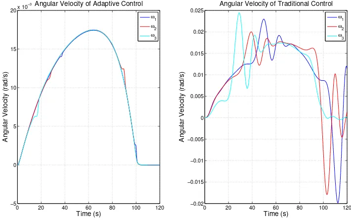
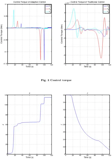
The angular velocity of the adaptive fault-tolerant control method and the traditional quaternion
feedback control method are separately shown in Fig. 1. The quaternion tracking is shown in Fig.
and Fig. 4 shows the adaptive parameters θ¯andδ¯against time, wherekθ= 107 andk
δ = 5×10³
is tuned experimentally for best performance. The traditional control method fails to perform the
required motion whereas the adaptive control performs the maneuver.
B. Simulation with Deviation Fault
To illustrate the nature of deviation fault, we set
d1=
0 t≤50s
0.01 t≥50s
(30)
0 20 40 60 80 100 120
0 0.005 0.01 0.015 0.02 0.025
Time (s)
Angular Velocity (rad/s)
Angular Velocity of Adaptive Control
0 20 40 60 80 100 120
−0.05 0 0.05 0.1 0.15 0.2 0.25 0.3 0.35
Time (s)
Angular Velocity (rad/s)
Angular Velocity of Traditional Control
ω
1
ω
2
ω
3
ω
1
ω
2
ω
[image:13.595.115.477.235.491.2]3
Fig. 5 Angular velocity
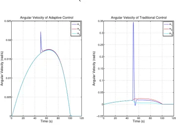
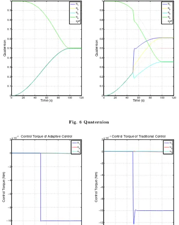
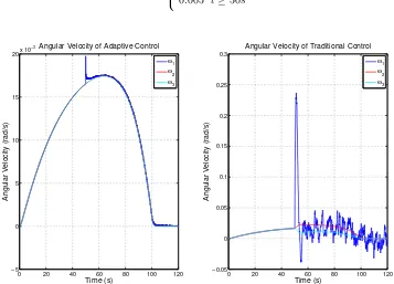
The angular velocity of the spacecraft using the adaptive fault-tolerant control and the
tradi-tional quaternion feedback control are separately shown in Fig. 5 and the quaternion tracking in
Fig. 6. Fig. 7 illustrates the control torque of the adaptive and traditional control. Fig. 8 shows
how adaptive parameter changes, where kθ = 103 and kδ = 500. From these gures, we can see
that when the actuator deviation fault occurs at 50s, the angular velocity on both control
meth-ods immediately deviate. In the case of the adaptive control method, the angular velocity quickly
responds and moves back to the desired reference while the traditional control method completely
0 20 40 60 80 100 120 0 0.1 0.2 0.3 0.4 0.5 0.6 0.7 0.8 0.9 1 Time (s) Quaternion
Quaternion of Adaptive Control
0 20 40 60 80 100 120
0 0.1 0.2 0.3 0.4 0.5 0.6 0.7 0.8 0.9 1 Time (s) Quaternion
Quaternion of Traditional Control
q 1 q2 q 3 q 4
qref
q 1 q2 q 3 q 4
[image:14.595.125.475.58.280.2]qref
Fig. 6 Quaternion
0 20 40 60 80 100 120
−12 −10 −8 −6 −4 −2 0 2x 10
−3
Time (s)
Control Torque (Nm)
Control Torque of Adaptive Control
0 20 40 60 80 100 120
−14 −12 −10 −8 −6 −4 −2 0 2x 10
−3
Time (s)
Control Torque (Nm)
Control Torque of Traditional Control
u 1 u2 u 3 u 1 u2 u 3
Fig. 7 Control torque
C. Simulation with Combined Actuator Faults
To show the ability of the adaptive control method in dealing with the actuator faults, both a
gain fault and a deviation fault are simulated. With the gain fault as
[image:14.595.115.483.68.531.2]0 20 40 60 80 100 120 1.715
1.72 1.725 1.73 1.735
1.74 ¯
θ
Time (s) ¯θ
0 20 40 60 80 100 120
3.3 3.35 3.4 3.45 3.5 3.55 3.6 3.65
3.7 ¯
δ
[image:15.595.121.478.59.280.2]Time (s) ¯δ
Fig. 8 Adaptive Parameters
whererand(t)is a random number between 0 and 1. The deviation fault is
d1=
0 t≤50s
0.005 t≥50s
(32)
0 20 40 60 80 100 120
−5 0 5 10 15 20x 10
−3
Time (s)
Angular Velocity (rad/s)
Angular Velocity of Adaptive Control
ω
1
ω
2
ω
3
0 20 40 60 80 100 120
−0.05 0 0.05 0.1 0.15 0.2 0.25 0.3
Time (s)
Angular Velocity (rad/s)
Angular Velocity of Traditional Control
ω
1
ω
2
ω
[image:15.595.121.478.405.662.2]3
0 20 40 60 80 100 120 0 0.1 0.2 0.3 0.4 0.5 0.6 0.7 0.8 0.9 1 Time (s) Quaternion
Quaternion of Adaptive Control
q 1 q2 q 3 q 4
qref
0 20 40 60 80 100 120
0 0.1 0.2 0.3 0.4 0.5 0.6 0.7 0.8 0.9 1 Time (s) Quaternion
Quaternion of Traditional Control
q 1 q2 q 3 q 4
[image:16.595.125.476.58.280.2]qref
Fig. 10 Quaternion
0 20 40 60 80 100 120
−12 −10 −8 −6 −4 −2 0 2x 10
−3
Time (s)
Control Torque (Nm)
Control Torque of Adaptive Control
u 1 u 2 u3
0 20 40 60 80 100 120
−10 −8 −6 −4 −2 0 2x 10
−3
Time (s)
Control Torque (Nm)
Control Torque of Traditional Control
u 1 u
2 u3
Fig. 11 Control torque
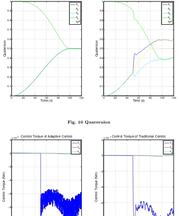
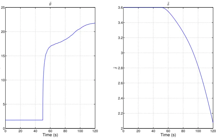
The angular velocity of the adaptive fault-tolerant control method and the traditional quaternion
feedback control method are shown in Fig. 9. The quaternions are shown in Fig. 10. Fig. 11
illustrates the control torque of the adaptive control method and the traditional control method,
[image:16.595.115.483.67.513.2]0 20 40 60 80 100 120 0
5 10 15 20
25 ¯
θ
Time (s) ¯θ
0 20 40 60 80 100 120
2 2.2 2.4 2.6 2.8 3 3.2 3.4
3.6 ¯
δ
[image:17.595.130.477.58.282.2]Time (s) ¯δ
Fig. 12 Adaptive Parameters
kθ = 107 andkδ = 3×10³. From these gures, compared with the traditional quaternion control
law, the adaptive fault-tolerant control law demonstrates a good control performance relative to the
conventional controller (28) and reaches the desired state.
V. Conclusion
Two kinds of spacecraft actuator failures were considered: a gain fault, and a deviation fault.
An adaptive fault-tolerant control method is proposed for the spacecraft experiencing these actuator
failures. The fault-tolerant control in this paper relies on an ideal reference model to identify when a
fault occurs. The control tracks the ideal reference model to replicate it as closely as possible. This
control employs adaptive parameters to improve the responsiveness of the angular velocity error
and the quaternion error due to actuator faults. Moreover, the angular velocity error magnitude is
more sensitive than the quaternion error to an actuator fault. This sensitivity can be exploited in
the control design by more aggressively tracking the angular velocity of the ideal system relative to
the quaternion error. This is achieved by introducing time-dependent parameters that weight the
components of the feedback control respectively. In the case of a gain fault (and stuck fault) the
improve the performance over a conventional control in the presence of these actuator faults.
Acknowledgments
This work is partly supported by the Chinese Scholarship Council.
References
[1] K. L. Bedingeld, R. D. Leach and M. B. Alexander, Spacecraft System Failure and Anomalies At-tributed to the Natural Space Environment, NASA Reference Publication, 1996, pp.1390.
[2] M. Tafazoli, A Study of On-orbit Spacecraft Failures, Acta Astronautica, Vol. 64, 2009, pp. 195-205, DOI: 10.1016/j.actaastro.2008.07.019.
[3] X. Huo, Q.L. Hu, B. Xiao, Finite-time Fault Tolerant Attitude Stabilization Control for Rigid Space-craft, ISA Transactions, Vol. 53, 2014, pp. 241-250.
[4] W.C. Cai, X.H. Liao, Y.D. Song, Indirect Robust Adaptive Fault-Tolerant control for Attitude Tracking of Spacecraft, Journal of Guidance, Control, and Dynamics, Vol. 31, No. 5, 2008, pp. 1456-1463, DOI: 10.2514/1.31158.
[5] B. Jiang, Z.F. Gao, P. Shi and Y.F. Xu, Adaptive Fault-Tolerant Tracking Control of Near-Space Vehicle Using Takagi-Sugeno Fuzzy Models, IEEE Transactions on Fuzzy Systems, Vol. 18, No. 5, 2010, pp. 1000-1007, DOI:10.1109/TFUZZ.2010.2058808.
[6] K. M. Passino and P. J. Antsaklis, Fault Detection and Identication in an Intelligent Restructurable Controller, Journal of Intelligent and Robotic System, Vol.1, 1988, pp. 145-161.
[7] R. Marino, Adaptive Control of Nonlinear Systems: Basic Results and Applications, A. Rev. Control, Vol. 21, 1997, pp. 55-66.
[8] B. Wie and P. M. Barba, Quaternion Feedback for Spacecraft Large Angle Maneuvers, Journal of Guidance, Control, and Dynamics, Vol. 8, No. 3, 1985, pp. 360-365, DOI: 10.2514/3.19988.
[9] B. Wie, Space Vehicle Dynamics and Control Second Edition, American Institute of Aeronautics and Astronautics, 2008, pp. 426-428.
[10] O. Egeland and J. M. Godhavn, Passivity-Based Adaptive Attitude Control of a Rigid Spacecraft, IEEE Transactions on Automatic Control, Vol. 39, No. 4, 1994, pp. 842-846, IEEE Log Number: 9216442.
[12] Y. Han, J. D. Biggs and N.G. Cui, An Application of Adaptive Fault-Tolerant Control to Nano-Spacecraft, 2nd Conference on Dynamics and Control of Space Systems, Rome, 2014.
[13] C. Maclean, D. Pagnozzi and J. D. Biggs, Planning Natural Reporting Manoeuvres for Nano-Spacecraft, IEEE Transactions on Aerospace and Electronic Systems, 2014, 50(3), 2129-2145. DOI: 10.1109/TAES.2014.130417.
[14] B. Wie, H. Weiss and A. Arapostathis, Quaternion Feedback Regulator for Spacecraft Eigenaxis Ro-tations, Journal of Guidance, Control, and Dynamics, Vol. 12, No. 3, 1989, pp. 375-380.
[15] D. Fragopoulos, M. Innocenti, Stability considerations in quaternion attitude control using discontin-uous Lyapunov functions, IEEE Proc.- Control Theory Appli., Vol. 151, No. 3, 2004, pp. 253-258, doi: 10.1049/ip-cta:20040311.
[16] J. Biggs, N. Horri, Optimal Geometric Motion Planning for a Spin-Stabilized Spacecraft, Systems and Control Letters, Vol. 61, No. 4, 2012, pp. 609-616.
[17] C. P. Tang and C. Edwards, Sliding Mode Observers for Robust Detection and Reconstruction of Actuator and Sensor Faults, Int. J. Robust and Nonlinear Control, Vol. 13, 2003, pp. 443-463, DOI: 10.1002/rnc.723.
[18] L. Psiaki, Magnetic Torquer Attitude Control via Asymptotic Periodic Linear Quadratic Regulation, Journal of Guidance, Control, and Dynamics, Vol. 24, No. 2, 2001, pp. 386-394.
[19] B. T. Costic, D. M. Dawson and M. S. de Queiroz et., Quaternion-Based Adaptive Attitude Tracking Controller Without Velocity Measurements, Journal of Guidance, Control, and Dynamics, Vol. 24, No. 6, 2001, pp. 1214-1222, DOI: 10.2514/2.4837.
[20] J. T.Y. Wen and K. Kreutz-Delgado, The Attitude Control Problem, IEEE Transactions on Automatic Control, Vol. 36, No. 10, 1991, pp. 1148-1162.
[21] Z.X. Li and B.L. Wang, Robust Attitude Tracking Control of Spacecraft in the Presence of Dis-turbances, Journal of Guidance, Control, and Dynamics, Vol. 30, No. 4, 2007, pp. 1156-1159, doi:10.2514/1.26230.