This is a repository copy of Data visualization and health econometrics.
White Rose Research Online URL for this paper: http://eprints.whiterose.ac.uk/120147/
Version: Accepted Version
Article:
Jones, Andrew Michael orcid.org/0000-0003-4114-1785 (2017) Data visualization and health econometrics. Foundations and Trends in Econometrics.
https://doi.org/10.1561/0800000033
Reuse
Items deposited in White Rose Research Online are protected by copyright, with all rights reserved unless indicated otherwise. They may be downloaded and/or printed for private study, or other acts as permitted by national copyright laws. The publisher or other rights holders may allow further reproduction and re-use of the full text version. This is indicated by the licence information on the White Rose Research Online record for the item.
Takedown
If you consider content in White Rose Research Online to be in breach of UK law, please notify us by
Data Visualization and
Health Econometrics
*
Andrew M Jones
Professor of Economics, Department of Economics and Related Studies, University of York, Heslington, York, YO10 5DD, United Kingdom
Abstract
This article reviews econometric methods for health outcomes and health care costs that are used for prediction and forecasting, risk adjustment, resource allocation, technology assessment and policy evaluation. It focuses on the principles and practical application of data visualization and statistical graphics and how these can enhance applied econometric analysis. Particular attention is devoted to methods for skewed and heavy-tailed distributions. Practical examples show how these methods can be applied to data on individual healthcare costs and health outcomes. Topics include: an introduction to data visualization; data description and regression;
generalized linear models; flexible parametric models;
semiparametric models; and an application to biomarkers.
*
Contents
1. Introduction
2. Data Visualization Ð a Primer
3. Methods
3.1 Data Description and Regression
3.2 Generalized Linear Models
3.3 Flexible Parametric Models
3.4 Semiparametric Models
3.5 Distributional Methods
4. An Application to Biomarkers
5. Conclusion
Appendix
A.1 Web resources
1
Introduction
Econometric models for health outcomes and health care costs are used for prediction and forecasting in health care planning, risk adjustment by insurers and public providers of health care, geographic resource allocation, health technology assessment and health policy impact evaluations. Methods for risk adjustment focus on predicting the treatment costs for particular types of patient, often with very large survey or administrative datasets.
In the recent literature attention has shifted away from linear regression models to semiparametric and flexible parametric estimators. A popular semiparametric approach is to use generalized linear models or GLMs (e.g., Buntin and Zaslavsky, 2004; Manning and Mullahy, 2001; Manning et al., 2005; Manning, 2006). GLMs are built around a link function that specifies the relationship between the conditional mean and a linear function of the covariates and a
distributional family that specifies the form of the conditional variance as a function of the conditional mean. GLM models are estimated using a quasi-likelihood approach derived from the quasi-score or Òestimating equationsÓ.
In a conventional GLM the choice of link and distribution has to be specified a priori. In practice the most frequently used GLM specification for medical costs has been the log-link with a gamma variance (Blough et al., 1999; Manning and Mullahy, 2001; Manning et al., 2005). Basu and Rathouz (2005) have developed a flexible semiparametric approach to the problem of selecting the appropriate link and variance functions. Their extended estimating equations estimator (EEE) approach uses a Box-Cox transformation for the link function and either a power variance or quadratic variance function for the distribution. The particular form of the link and distribution are thereby estimated from the data at hand.
Other semiparametric methods that have appeared in the literature on modelling health care costs include the conditional density estimator and finite mixture models. The conditional density approach was advocated by Gilleskie and Mroz (2004) and divides the support of the distribution of the dependent variable into discrete intervals then applies discrete hazard models to these, implemented in practice as a series of sequential logit models. Finite mixture models use a discrete mixture of parametric models and, for example, have been applied to medical costs by Conway and Deb (2005). Combining simple distributions such as the gamma or log-normal in a mixture of relatively few components may approximate complex empirical distributions effectively, especially for distributions that are multi-modal.!
beta distribution of the second kind (GB2). This provides the additional flexibility to fit the high level of skewness and the heavy tails seen in cost data (Jones et al., 2014). The downside of this flexibility is a risk of over-fitting and, in practice, these approaches may be best used as a guide to selecting one of the special or limiting cases that are nested within the general models. In this respect the flexible parametric models can play a similar role to using the EEE approach to select the link and distribution functions to be used in a GLM.
Earlier literature reviews have synthesised and compared the wide range of approaches to modelling health care costs (e.g., Hill and Miller, 2010; Jones, 2000, 2011; Jones et al., 2013; Mullahy, 2009). In addition, studies using a quasi Monte Carlo design, based on English administrative data for patient level costs of hospital care, have provided an assessment of the relative performance of these approaches (Jones et al., 2014, 2015, 2016). To complement these earlier studies this article focuses on the principles and practice of data visualization and statistical graphics and how these can enhance empirical analysis of health care costs and outcomes, especially for skewed and heavy-tailed distributions. The scope of this review is limited to non-normal but continuous outcomes such as health care costs and biomarkers. Many health economics applications deal with categorical and ordered outcomes, count data, or duration data. Methods for these are reviewed in Jones (2000) and Jones et al. (2013). The methods and applications used here are limited to cross sectional data. For discussions of methods for panel data see Jones (2009) and for the use of cohort data (Von Hinke Kessler Scholder and Jones (2015).
Practical examples show how these graphical methods can be applied using the software package Stata, which is widely used in applied econometrics. Stata is not the obvious software of choice for specialist work in data visualization especially for users who wish to present their work online and to make use of animation or interactivity. Nevertheless, for many applied econometricians it is the workhorse for data management and econometric analysis. In this article Stata code, shown in the font courier new, is included to show how far it is possible to go within Stata so that graphical analysis can be integrated with statistical and econometric analysis within one piece of software and using one set of syntax.
2
Data Visualization Ð a Primer
ÒGreatest number of ideas in the shortest time with the least ink in the smallest spaceÓ
Edward Tufte (1983)
Edward TufteÕs ideas, expressed in his 1983 book The Visual Display of Quantitative Information and in subsequent publications, have been highly influential in the field of data visualization (Tufte 1983, 1990, 1997, 2001, 2006). Tufte has developed a set of principles of graphical excellence which are summarised here:
- Show the data.
- Induce thought about substance (not methods, visual style…).
- Do not distort the data.
- Present many numbers in a small space.
- Make large data coherent.
- Encourage the eye to compare.
- Reveal levels of details Ð from overview to fine structure. - Serve a clear purpose (whether it be description, exploration,
decoration, etc).
It is clear that this perspective favours functionalism, minimalism and clarity of design over embellishment and visual ÒfireworksÓ. TufteÕs influence is evident in the recent article by Jonathan Schwabish (2014) in the Journal of Economic Literature, ÒAn economistÕs guide to visualizing dataÓ, which aims to bring TufteÕs philosophy of graphical design to an economics audience by critically appraising and redesigning graphics that have appeared in articles published in the American Economic Review.
In addition to Edward TufteÕs work other sources for the ideas and material presented in this brief primer include the books of Stephen Few (2009, 2012, 2013, 2015) which share the same focus on simplicity of design and clarity of purpose but with a more pragmatic approach aimed at those providing business information in tabular and graphical formats. FewÕs web page, Perceptual Edge, provides a useful source of case studies and critical appraisals of published visualizations (see the Appendix for information on this and other web links that are relevant sources of ideas for data visualization).
Nathan YauÕs blog Flowing Data and his books Visualize This and Data Points (Yau, 2011, 2013) provide a visually elegant and contemporary guide to good practice that is rooted in statistical analysis with an emphasis on online resources and interactive graphics.
Alberto Cairo (2012, 2016) comes from a background of experience in data journalism and working with infographics. His books The Functional Art and The Truthful Art draw on the lessons of cognitive psychology and their implications for graphical design. Jorge CamoesÕs (2016) Data at Work shares a similar perspective. It provides an impressive glimpse of how far Microsoft Excel can be taken to produce effective and visually appealing graphics.
Lessons for statistical graphics from the psychology of visual perception are tested and put into practice in a classic article by Cleveland and McGill (1984) and are covered in a book by William Cleveland (1985)
The Elements of Graphing Data. These lessons are put into practical form by Naomi Robbins (2005) in her book Creating More Effective Graphs.
corresponding code alongside. MitchellÕs Guide is complemented by an encyclopaedic source of the various forms of statistical graphic that have been used in practice across a broad range of disciplines in Robert HarrisÕs (1999) Information Graphics: A Comprehensive Illustrated Reference.
One feature of Mitchell (2012) is to stress the usefulness of graphics schemes in Stata. Schemes are text files that can be called upon to set options that affect the appearance of Stata graphics. This saves having to add numerous sub-commands when using individual graphics commands. The default colour graphics scheme used by Stata is called s2color, which can be set explicitly using:
set scheme s2color
Many other schemes are available. For example to adopt the visual style of the Economist magazine use:
set scheme economist
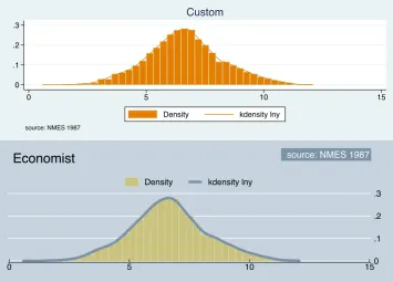
Alternatively a custom written scheme can be created and installed. The graphics illustrated in this article were mainly done using a very simple custom scheme that begins by including the default scheme and then modifies some of the colour options that are used by default to give a palette based on dark orange:
#include s2color
color background ltbluishgray color histogram dkorange
color boxplot dkorgange color p2 dkorange
color bar dkorange color hbar dkorange
Fig 2.1 Histograms drawn with different schemes
Returning to Edward Tufte. Following his principles of graphical excellence, Tufte (1983) has identified many of the pitfalls that can arise when visualisation is done badly. These include:
Distortion: when a graphic creates a distorted picture of the underlying data. For example if the angles in a pie chart or the areas in a histogram do not match the variation in the data. A classic example is the way in which a non-zero baseline in a bar chart can be used to create a biased impression of the difference between the height of the bars.
Design variation: when the visual features of a graphic, such as shading or colouring do not match the variation in data that is being represented. The implication is that in good visual design the graphical variation - whether it is differences in the position of points, lengths of lines, size of areas or differences in shading or colour - will reflect and illuminate the underlying statistical variation in the data and hence will make the variation visible and Òencourage the eye to compareÓ.
ÒChartjunkÓ: which is essentially the use of uninformative embellishment in graphics, such as the vibrations and grid patterns
0 .1 .2 .3
0 5 10 15
Density kdensity lny
source: NMES 1987
Custom
0 .1 .2 .3
0 5 10 15
Density kdensity lny
that are sometimes used to fill bars in a bar chart. A notorious example is the use of 3-D effects in graphics, such as bar charts, where the addition of 3-D typically reduces the clarity of the graphic.
Lack of content: where excessive space is devoted to graphing relatively little quantitative data. This is the antithesis of TufteÕs call to present many numbers in a small space. In these cases tabulating may be more effective than graphing the data.
To put these ideas into practice and to help sift effective from ineffective graphics, Tufte (1983) introduced a couple of simple concepts that can be used to evaluate a graphic: the data-ink ratio
and the data density. Data ink corresponds to marks on the page that
represent data points, such as the dots in a scatter plot, while the remaining non-data ink represents all the other marks, which may be functional such as titles, labels, axes, gridlines and tick points or may be purely decorative. So:
Data-ink ratio = data ink/total ink
Implicit in this concept is the notion that the data-ink ratio equals one minus the proportion of ink that could be erased without loss of statistical information and that the design of a graphic should aim to minimize non-data ink. In practice there are limits on how far this can be taken as non-data ink often helps the eye to navigate and interpret a graphic and may help to make it eye-catching and memorable.
The data density takes the number of data points that are being graphed relative to the physical size of the graphic to capture the principle of aiming to present many numbers in a small space:
Data density = number of entries in data matrix area of data graphic
Tufte has suggested a related concept: the Shrink principle that Ògraphics can be shrunk way downÓ and that readers can cope with quite small graphics and with multiple graphics presented alongside each other. This principle is embodied in the use of information dashboards to combine multiple graphical and tabular views of data in a single dashboard format (Few, 2013).
Tufte is not alone in taking a prescriptive approach to visualization. Cairo (2016) also provides a couple of ÔchecklistsÕ to guide practitioners. In the first he argues that Òa good visualization is:
- reliable information;
- visually encoded so relevant patterns become noticeable;
- organised in a way that enables at least some exploration,
when itÕs appropriate;
- and presented in an attractive manner, but always
remembering that honesty, clarity and depth come firstÓ.
In the second, influenced by Enrico Bertini, Cairo (2016) argues that the qualities of a good chart are:
- It is truthful (based on thorough and honest research). - It is functional (accurate depiction of the data).
- It is beautiful (pleasing for audience). - It is insightful (reveals evidence).
- It is enlightening(changes minds for the better).
To illustrate how Edward TufteÕs ideas might be put into practice start with a histogram of individual data on annual medical costs. These data are from the 1987 US National Medical Expenditure Survey (NMES). Data that have been used as part of the evidence surrounding tobacco litigation in the United States and in analyses of the health care costs attributable to smoking (Rubin, 2001; Johnson et al., 2003; Imai and Van Dyk, 2004). The dataset used here includes total annual health care costs measured in US dollars, measures of smoking that include indicators for current, ex- and never smokers and a variable for pack years, the product of years of smoking and packs per day, along with controls for age, sex, education, marital status, poverty status and region1.
In Figure 2.2 the top left-hand panel shows the histogram for the logarithm of medical costs that is produced using the Stata default graphics settings. To modify these the top right-hand panel removes
1
the axis lines, which are non-data ink, and rotates the labels on the axis to make them more legible, while adding a note of the data source. The bottom-left panel takes the elimination of non-data ink a step further by removing the grid lines while keeping them as a reference point by superimposing white lines over the shaded area of the histogram and by removing the axis label. This process of elimination could have been taken further. For example, the shading of the bars is non-data ink and could be eliminated to leave hollow outlines, or simply horizontal lines to mark the height of each bar. In practice the elimination of non-data ink typically reaches a point where further simplification hampers the legibility of a graphic and here the process stops at shaded bars. In this case the purpose of the histogram is more qualitative, to give an impression of the overall shape of the distribution - is it symmetric, unimodal, heavy tailed? - rather than to read off precise quantitative information about the height of the density at different points. So the qualitative contrast between the shaded bars and the white background serves this purpose well. Finally, the bottom-right panel adds some further information by super-imposing a kernel density plot to smooth out the outline of the distribution.
Fig 2.2 Refining the histogram
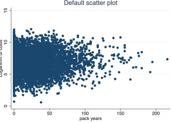
Now consider the default version of a scatter plot produced in Stata. Figure 2.3 shows the logarithm of annual health care costs plotted
0
.1
.2
.3
D
e
n
si
ty
0 5 10 15
Logarithm of costs
0 .1 .2 .3
D
e
n
si
ty
0 5 10 15
Logarithm of costs source: NMES 1987
0 .1 .2 .3
0 5 10 15
source: NMES 1987
0 .1 .2 .3
0 5 10 15
against a measure of individual smoking history based on pack years and reveals their joint distribution through the density of data points. This was produced and saved as an encapsulated postscript (eps) file to be used for publication. This is a vector graphics format which, like pdf format, is scalable and should look sharp at any size. This is an alternative to raster graphics formats such as tif, jpeg and gif files. The following code is used:
tw scatter lny treat, title(Default scatter plot) name(scatter, replace)
[image:15.595.127.474.302.552.2]graph export scatter.eps, replace
Fig 2.3 Scatter plot of log(costs) and pack years
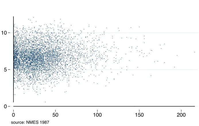
One way to reduce the proportion of non-data ink used in this standard scatter plot is to replace the standard horizontal and vertical axes by a range frame plot so that the length of the lines that appear on the axes represent the range of the y and x variables and hence become data themselves. This is show in Figure 2.4. Note that the default scatter of ÔdotsÕ has been replaced by a cloud plot so that individual data points become visible and better represent the use of microdata and the extensive heterogeneity that is typical of such data. Also the tick points on the vertical axis have been rotated so
0
5
1
0
1
5
L
o
g
a
ri
th
m
o
f
co
st
s
0 50 100 150 200
that they are easier to read. In this case using the range on the horizontal axis does not really add much but the vertical axis does reveal the limits on the range of the logarithm of costs.
Fig 2.4 Range-frame plot of log(costs) and pack years
The range-frame plot was drawn with the following code where the axes are drawn as functions:
tw (scatter lny treat, msymbol(p) legend(off) ylabel( , angle(horizontal)) )
(function y=0, range(0 216) lcolor(black))
(function y=0, range(0.57 12.2) lcolor(black) horizontal), title(Range frame plot)
ysca(noline) xsca(noline) name(rangeframe, replace) note($note)
A more informative alternative to the range frame plot is a dot-dash
plot where the marginal distributions of y and x are shown using dashes for individual data points. Figure 2.5 reveals detail in the tails of these marginal distributions rather than just showing the overall range of the data so that the horizontal axis now becomes
0 5 10 15
0 50 100 150 200
source: NMES 1987
informative as well as the vertical. In particular the skewness and sparsity of the observations in the right-hand tail of the distribution of pack years is revealed.
Fig 2.5 Dot-dash plot of log(costs) and pack years
The dot-dash plot was produced using the following code where the axes are drawn using scatter plots:
* Dot-Dash plot gen where_x=0 gen where_y=-6 gen pipe = "|" gen bar ="_"
tw (scatter lny treat, msymbol(p) xsca(noline) ysca(noline) legend(off)
(scatter where_xtreat, ms(none) mlabel(pipe)) (scatter lny where_y, ms(none) mlabel(bar)),
note($note) title(Dot-Dash plot) name(dotdash, replace) || | | | | | | | || | | | | |||| | |||| | | | || | | | | |||||| | || | | | | | | || | |||| | | | | | |||| | ||||| | |||| | | | | | |||| | | | |||| | | | |||| | |||||||| | | || || | | | | || || | | | | | | | | | | | | | | || | | | | | | | || || | | || | ||||| | || | | || | | | || | || | | | | | | | | || || | | || | | | | | | | || | || | ||||||| | | | || | | || | | || | || | | | |||||||| || | || ||| | | ||| | | | | || | |||||| | | | | | | |||| | | | | || | || ||| | || | || | || | | | || | | |||| | || || | | | | || ||| | || | | | | | || | ||| | | | || || || | | | | | | | | || | | || || || | | | ||| | | | | | ||| | ||| | || | |||| | | | | | | | | | | | || | | | | | | | |||| | | | |||| | ||||| | || | | | | || | || | | || | || || | ||| | | | |||| | | || | | | || | | | ||| | ||| | || | | | | | | |||| | | | | ||||| | | | | | | |||| || || | | | || | | || | ||||| | || | |||||| | | || | | | | | | ||||| | | | | |||| | | | || | ||| | | | | | || | | ||||| | | | | | ||||||| | | | | | | | || | | || | | | | | | || | |||| || | | | | || | | | || | | | | | | ||| | | | | | || ||| | || |||| | | | | | | | | | | | | | | | | | ||| | ||||| | | | |||| || |||| | | | | | | | ||| || | | | || | | | || | || |||| | | ||| | | ||| | | | | ||| | | | | |||| | | | | ||||||| | | | | ||| | | | | | | ||| | || | | | | | | | | | || | | | | || || | || || ||||| | | | | | | | |||| | | | || | || | | | | | | | | | ||| ||||| || | | | | | |||| | | | | || | | | ||| | | || | | | | | | | ||| || | | | | | | || | || | | | | || | | | | | || | | | | | | | | | || || | | | || | | | | | | | || | | | || | | | | | | | || | | | | | | | | | | ||| | | | | | |||| | | | | | | | || | | || | | | | | ||| | | | || | || | | | | | || | | | | | | || | || | | | | | |||| | | | |||| | | | | | | | | | | | ||| | | |||| | | | | | | | | | | | | | | | | ||| | | | || | | || | | | | | | || | | | | | || | | | || | | | || | ||| | | || | ||| | || | || | | | | | | ||||| ||| | | |||| | | | | | ||| | | | || | | ||| | || | | | | | | || | | | | | | ||| | ||||||||||||||||| | | | | || | | | | | | | | | | ||| | | | | || | | | | |||| | | ||| | | | | | |||| | ||| || | | | ||| | || | | ||| | | | | ||| || | | | | | | | | | | ||| | | | | | | | | | ||| || | | || | | | | | ||| | || | | ||||| | ||||| || | ||||| | || | | || | || | | | | | || | | | | | | | | ||| | |||||| | | | | | | || || | | | || || | || | | | || | | | || | | | | |||| | | | | | | | | | |||||| | ||| || | ||| | | || | | | | | || | || || | | | | | | | | | | | | | | | | |||| | || | | || | | | | |||| | | || | | || | | ||||| | | | | | | | | | | | | | | | | | | | | | | | | | | | ||| | |||| | || | | | | | ||||| | || | | | | | | || | ||| | | | | | | | | | | | ||| | | |||||| | | | | | | | ||||| | |||| | ||| | | || | | || | | | | | | | || | | ||| | | | | | | || | | ||||| | | ||| | | | |||| | | | | | || | | | | | | | | | | | ||| | | ||||| | | | | | || | || | | | || | | || | ||| | || | ||| | || ||| | ||| | ||| | || | | | | | | | | | | | | | | || | | | | | |||| | | | || | | ||||||||||||| | | | | | |||| | || | ||| | | ||| | || | | | | | | |||| | || | | | |||||| | |||| | | | | | | | || | ||| | | |||| | | | ||| | | | | | | | | | | | | | || | | | | | | | || | | | |||| | | | | | | | | || | | | | | | | ||| | ||| | | | | || || || || || | ||| | |||| | | | | | | | | | || | ||| | | | | | | || | | | ||||| | ||| | || | |||| | || | ||||| ||| || | | ||||||| | || | || | | | | | | || | | | || | ||||| | | | | | | | | | | | | | | ||| | | | |||| | || | | | | || | | | | | | | | || | | | || || | | | ||| || | ||| | | || | | | | | | | |||| || || | | || | || | || | || || | | | | || ||||| | || | | | ||||| | | || | | | ||| | | | | || | | | | |||||| | ||| || || | | | | ||| | | | | | | | | | | | ||| || | ||| | || || | | | | | | | | | | | | | | | |||| | | ||| | | | ||| | | | ||| | || | | | | | |||| | || | | || | | | | | | | | ||||| | | | | | | | | | || | || | | | | | | | ||| | | | || || | | | | | | | | | || | || | ||| | | || | | | | | | | | | | ||| | || | | || || | | | | | ||| | || | | | | ||| | | | | || | | |||| | |||||| ||| | ||| | |||| | | |||||| | | | || | | | | | | | || | | || | | || | | || | ||||| | | || | || || || | || | | || | || || | | | | | | | ||| | | | | | | | | || | | || || | | || ||||| | ||||| | ||| | | | | | | || | || | | | | | | | | ||| | || | | | | ||||| || || | ||| | ||| | | | | || | | | | ||| | |||| | |||||||||| | | | ||| | || | |||||||||| | | ||| | || | | | | ||| | |||||| | || | | | | || | ||| | | | | | ||| | ||| | | | || | | | | || | | | || | | || | | | | ||| | | | | | | | | ||| | || | | || | ||||| |||| | || | ||| || | | | | | | | || | | | | | | ||||| | |||| |||| | || || | ||| | | || | | | || || | | | | | |||||| ||| | | | | | || |||||||| ||| | | | | | ||| | || | | ||| | | | | || | ||| | || | | | | ||| ||| | | | || | |||| | | | | ||||| || | | |||| | || | | ||||| | | | | | | || | | | | | | | |||| | ||||| | | | | | || | | | || | | | | | | | | | | | || | | | |||| | ||||| | | | ||||| | || | | ||| | | | | | | | | | | | || | | | ||||| | | |||| | | | ||| | ||||| | | || | | | | | ||| | || | | || | | | | | | | | | | || | | | | | | | ||| | | | | || | | | |||| | | || | | |||||| | ||| | || | | || | | | | |||| | |||| | |||| | | | | | | | | | | | || | | | | | | | | | | | | || | | | | ||| | | | | ||| | ||| | | | ||| | |||||| | |||||| | |||| |||| | || | || | | | |||| | | || | | | | | ||||| | ||| | | | | | | | ||| | | | | | || | | || | || | | || | ||||||||||||| || | || | | | | | |||| || | ||| | || | || ||||| | | | | || | | | | | | | | | || | | | | | | || || | | | | || | | | | |||| | ||| | ||| | ||| | | | | || | || | | ||| | | || | | | | | | | | || | | | | | || | | || ||||| | || | |||| | | | |||||| | | ||| | | | ||| | | ||||||| | | | | || | || | | ||||||| | | |||||| | || | | | ||||| | || | | || | ||| | | ||||| | | | | ||| | | | | | | | || | | | | ||| | || | | | | | ||||| | || | ||||| | ||||| | |||||| | | || | | || | ||| | | | | |||| | | ||||||| | || | | | ||||| | ||||| | || | | | | |||| | | | | | | | ||||| | | | || | | | | | || | | | | ||| | | || | | | ||| | |||| | || | ||| | ||||| | | |||| | || ||| | || || | | | | | | | | | | ||| ||||| || || | | | || || | || | || | | | || || | | | | | || | | | | | || | | | | | | | | | | || | || | | | || | ||| | | | | | | ||| | | | || | | | || | | | | | | || | || | || | || | |||| | |||||| | | | | | | | | | |||| | | | | | || ||| | | | ||||||| || | | | | | | | ||| | ||| | | || | ||| | || | | | | || ||| | || | | | | | | | | | | || | || | | || | | || ||| || || | |||||| | | || | | | || | | | || | || || | || | | | | | | | | || | | | | | |||| | | | | || | ||| | | | | | ||| | | |||| | || || | | | ||| || | | ||| || || || | |||| | || | | | |||| | | | | | | | | || | | ||| | | || || | | | | | | | ||| | | | | ||| | ||| | | | || | | | | | | ||| | |||| | |||||| || ||| | | ||| |||| | | | | || | || | | | || | | || | || | |||| |||| || | | || | | | | | | | | | | | || | | || ||| | | | | | ||| | | | | |||| | | ||||| | || | | | | || | | | | || | | | | | | | | || | | || | |||| | ||| | || | ||| | || | || || | | || | | | | | | ||| || | | | ||| | | | || | | | | || | | | | | || || || | | |||||||| | ||| | | | | | | ||| | | | | | | | | | ||| | ||| | || | || | | | | | | | |||| | || | | | || | | | ||| | | | | | | | | | | ||| | | || | || | | | ||| | | | | | | || | || | ||| | | || || | | | | | | | | | | | | | | | | | ||| | | || | | |||| | | || | || | || | | | | | | | | | || | | | | | | | ||| | | | | | || | || | ||| | || |||| | || | | | || | | | | | | || | | | | || | | || | | | | || | | | | |||| | | | | ||| | ||||| || | | | | | | | | | | | | | | | || |||| | ||||| | | | || | | | || | | | | | | || | | | | | | ||| | | | | ||| | | | | | | | | || || | ||| | | | | | | | ||| | || ||| | | | | | || || || || | ||| | | | | | | |||| | | ||| | | | || | | |||| | || | | | | | | |||| | | | |||| | | | | |||| | | | | | | || | | | | | | | | | ||||| || | | | | || | | | | | | | || | | | | |||| | |||| | || | | | ||| ||| | ||||||||||||| | | || | |||| | | | | | | |||| | || | | | | | || | | |||| | |||||| | | |||| | ||| | | | || | | || | | | | | |||||| | ||||| | ||| | | | | | || | | | | | | | || || | | | || | | | | | || | | | | | || | | || || | | | | | ||||| | || | ||| | | | | | | | || | | || | | | | | | | | | | | ||| | | | | | || | | | || | | | | | | | |||||| | | ||||||| | | | | | | | ||| | || | || | | | | | |||| | | || || || | | | | || | || | | | | | | | | || | | | || | || | |||| | | | | | || | | | | | ||| | | || | | | | | || | | ||||| | | |||| | || |||| | | | | ||||||| | | | | | || | | ||| | | | | || | | | | | |||||| | ||| | || | | | || || | | | | | | || | || | | || | | | || || | | | | | | | | | | | |||| || | | || | | | || | | | | || | | | | | || | | | | | | | || ||| | | ||| | | | | || | | | | | | || | | | | | || | | | | | | | | | | ||||||| | || || | || | | | | || | | |||| | | | | || | | | | | ||||| | | || | | |||| ||| || | | | || | | | | ||| | | ||||| | | ||| | | | | | | || | || | ||| | || || ||| | ||| | | || || | | || | | | | || | || | | | | | | | | | || | |||||||| | | | | | || | || | || || || | |||| | ||||| | | || ||| | |||||| | | || | ||||||| | | |||||| | | || | |||||| | ||| | | || | | | || | | | || ||| | | | || | || | | | |||||| | || | ||| | | | ||| | | | | | | ||| | | | | | | | | | ||||||||| | || | ||| | | | | | || | | | ||||| | | | | | | ||||| | | || | | ||||| | || | || | | | ||| | || | || |||||||| | | | | | ||||||| || | || | ||| ||| | || | | | |||||| || | |||| || | || | | | ||||||||||| || | ||||| | ||| | || | | | | | | | | || | | || | | || | | || | ||| | ||| | | || | | || | | | | ||| | | ||| | | | | | | | | | | | || || | | ||||||| | | | | | | | | | | | | | | | ||| | | | | | || | | || | | | | ||| | | | | | | | | |||| | | || | || | | | | | | ||| | | | | || | || | || | | | | | | ||||| | |||||||||| | ||| | || | | || | | | |||| | | | ||||| | | | | | |||| | | |||| ||| || || | |||| | || | |||| ||| | ||| | | | || || | ||| || | ||| | | | | | | | | || || ||| | || | | | || | | | | | | || | | | | || || | | | | || | | | |||| | | |||| | | | | | | | | || || | | | | | | | | | ||| | | || | ||| | | | | || | | | || | || | ||| || | | | | | | | | ||| | || | | ||| | |||| | || | | | | || | | || | ||| | | | | | ||| | | | | ||| | | || | | | | | | || | || | | | | || | | | || || || | || | | | || | | | | | | | | |||||||| | | ||| || | || | | | || | | | || | | | ||| | | | | || | | | | | || | | | | | | | || | || | | || | |||| | ||| | || | || || | | | | || | | | | | | | |||||| || | ||||||| ||| | | | | ||| | | || | | ||| | |||| | | | | | | | | ||| | || | | |||| | | | || | | || | | | | | | | | | | ||| | || || | | ||| | | | | | | | |||||||||| | || | | || | | ||||||| ||| | | | | | || | | | || | | | || | | | ||||| | | | | | |||||||| || | |||| | | | | | | | | | | | | | | | | | | ||||| | | | ||| | | | | | | |||| | |||| | | | | | || ||| | | | | | | | | | | ||| | | | | | || | | | | | || | | | | | | | ||| | | | |||| | | | | | | | | | |||| | | | ||||| | | | | || | | || | | | || | ||| | | | | | | ||||| | | | | | || | | | | | | || | | | | | || || || || | | | | | | | | ||| | | | | | ||| | ||| | | | ||| | |||||| || | | | | | | | || | | | | | | |||| || | | ||| || | || | | | | | | || | | | | || | | |||| | || | ||| | ||| | || | | | | | | | || || | | | | || | ||| | | | | ||| | | | | || | || | | || | | | | || | | | | | | ||| | | | ||| | | | | | |||||| | |||| | | | || | || | || | | | | ||| | | | | | || | | | | | ||| | | | | |||||| | | || | || | | || | | || | || | | | | | ||||| || | | | |||||| | | | | | | | | || | | | | || | | | | | || | | | | | | | ||| | | || | || | || |||| | | | | || | | || | | | ||| | | | | | | | || | || | || || ||| | | | | | | | ||| | | | || || | | | | | | || | | | | || | | || | || | | | || | | || | || | | | | || | | | | | | | | | | | | | | || | | | | | |||| | | | | | | | || | | | | || | | | || | | | | | ||||||| | | ||||| | | | | |||| | ||||||| ||| | | | | | | | |||| | || | || | | | || | | | | | | | | ||| | | | || | | || | ||| | ||||||| | | ||| | | | | | | | | | | | ||| || | || | || | | ||| | | | | || | | | || | | || | | | | | | | ||| | || | | | | | || | | | | | | | | | | | | | | | | | ||| | || | | | | | | | || | || || | || | | | | ||| || | | | | | || | || | | | ||| | | || | || | | | ||| | || | | || | | | || | || | | | | | | | | | | || | | | | ||| | | | | || | || | ||| | |||| | | | | || | | | || | | | | | | | || | | | | | | | | ||| | | || || || || || | | || ||| | ||| | ||| | | | | | | | | |||||| | || ||| | |||| | | | | | || | | | || | | | | ||| | | | | | | | | | | | | | ||| | | | | ||| | | | || | | | | | | || |||||| | | | ||| | || || || | |||| | | | |||||| | | | | | | | | | | || | | ||| | || | | | | | || | | | | | | | ||| | | | | | || | | | | ||| | | | | | ||| | | || | | || | | | || | | | ||||||| || | | | | | | ||| | ||| | | ||| | ||||| | | | | | | | | || ||| | | || | || | | | | | || | | | | || | ||| || || | || | | | | || || | | |||| || | | |||| | | || | | | | | || | | || | || | ||| | |||| | |||| | | || | | || | | | | | || | | || | | | | | | ||||| | | | | | || | | || | | | | |||| ||| | | | | | | | | || ||| | | | || | || | || | | |||||||||||||||||| | | | | | | | | || | | | ||||| | | | ||| | | | ||||| | | | || | || | | || ||| || ||| | | || | ||| | | | | || ||| | | | | ||| | | | | | | | || | ||||| | | || | || | | | ||| | | || | ||||| | |||| | || | | | |||| | | ||| | ||| || | | | | | | | || | | | | | | | | | | || | | | | | | | |||| ||| | | | ||| | | | | | ||||||| | || | ||| | ||||||| | || | ||||| | |||||||| | || | || | | ||| | | | | | | | | | | | | | | ||| | || | | || | | || | | | | | || | | || | | | | || | | | || | ||| | || || | | | || ||| | | | | | || | | | | ||| | | | | | | | | || | ||| | || | | | | | | ||||| | || | ||| ||||| | | | | | | | | |||| || || | || | | | | | | | ||||| | | || || | | | | | || | | | | | ||| | | ||||| | | | ||||||||||||| | | | |||||| | | ||| | | || | | | | || | | | | ||| | | | || | | | || | | || | | | | | | | | | | | || | | |||| | ||||| || | |||| | | | | | | | | | | | | | | || | | | | |||| | | || | |||||| | ||| | | | || | ||| | || | || |||| | | | | | | || | | | |||| | || | | |||| | ||| | || ||| | | | | | | || | | |||||| | | | | | |||| | | | | | || | ||| | | | | || |||| | || | || | | | | ||| | | | ||| | | | | | || || | || | || ||| || | || | | | | || | | | ||||| | | | | | |||| | | ||||| | | || | | ||| || | ||| || || | | || ||| | | | || | | | | | | | || | ||| | | | | | || | | || || | | | | | | | || | | || | | | | | | | | || | | | | | | | ||| | ||| | |||| | |||||| | | | || |||| || | | | || || | | | | | | || | | |||||| | | | | ||| || || | || | | | ||| | | ||||| | | ||| | | || | ||| | | | | | | |||||| | | | | | || | | | | | | | | | | | | || | | | | || | | | | |||| | | | || | | | || | | | || || | ||||| | ||| | |||| | | | | | | | |||||| | || || | | ||| | || | | | | | | |||| | | | | || || | | | | | || | ||| | | | || | ||| | | || | | ||| | || | | | || | | | | | | | | | || || | | | |||| | | | || | || | || || | | ||| ||| | | | | | | | | ||| | | | | | | | | || | || | || || | || | || | | | | | ||| | | | || | | || | || | ||| | | | | ||| | | | | | | |||| | | || | || | ||||| | | | | |||||| | | | | | | | | | | ||| | | | | || | | | || || | | || | ||||| | | | ||||| | | || | || | |||||||||| | | | || | | ||| | | | | |||||||| | | ||| | | | | | | | || | | || | | | | | || | | | | | | | | | | | | || | | | | | | | ||| || | | ||| | | | | | || || | |||||| | ||||| | |||| | |||| | | | ||||| | |||||| | || | | || | |||| | |||| | ||| | ||| | ||||| | || | | | |||||| | |||| | | | | | || | | | | | | | || | | | | | | | | || ||||||| | | | | | | | | | | | | | | || | ||| |||| | | | | || | | | | | | | | | |||| | | | ||| | | | | | | | || | | | | | | | | | | | | | ||| | |||| | | | | || | | | | | | | | | | | | | | || | | | | | | | | | | | ||| | || | | | | | | ||| | | | | || | | | | | | || | ||| | | | | || | | || | ||| | | | || | |||| | | | | | |||||| | | | || | || | | |||| | ||| | | ||| || | | | | ||| | | || || || | | || | | || | | | | | || | | | | | | | | ||| | | | | | | || | | | | || | | | || | |||| | | | | | ||| | ||| || | | | | | || | | | | || | ||| | ||| | | | | ||| | | || | || | | | || | || | || || || | | ||| | || | || | | | |||| ||| | || || | |||| | | | || ||| | | | ||| | | || | | | | | | | | | | ||||| | || | |||||||| | | || | | ||| | | | | | | | | | | | | | | | | | ||| | || || | | | | | | | || | | | | | | | | | | | | || || | | | | | | | | | || | | | | || | || | | || | | || || | | || | | | | | | || | | | | | | | | | | | | | | |||| | | | ||| | | | | | | | | ||| | ||| | | ||| | | || ||||| | | | | ||| | | | |||| | | |||||| | | | | || | | | | | | | | ||| | | | | | | | ||| | ||||| | |||| | || | || | | | | || | |||||||||| | ||| | | | | | | | | | | | | | || | | | | | | | |||| | |||| | ||| | || | | | || | | | | ||| || | || | | || | | | | ||| | | | | ||| | || || | | || | | || | || | | |||||||| | | | | | | | | | | | | | | | | | | || ||| | | | | | | || | | || | | | | ||| ||| | | | | | | | || | | | | | | | || | | | | | | | | | | | | | | | | | | | | | ||| | ||| | | | | ||| | | | | | | | || | | | | | | || | | | | ||| | | | | | | || | |||| | | |||| | ||| | | | | | | ||| | | ||||| | | | | ||| | | | || | || || | | || | | | |||| | | | | | | | | || | | | | |||||| | | | | | | | || || | | | | | | |||| | |||||| | || | || | ||| | | | | | | | | | |||||||| | | | | |||| | | | || | | || | | | | |||||| | | | | | | | ||| || |||| | | | | | | | | | ||||||||| | |||||| | || || | | || || | | || | | | ||| | || | | | | | | | | || | ||| | |||| | | | || | | ||| | |||| | | | | || | | | | ||| | | | ||| | | || | | | || | | | | ||| | | | | | | | | | || | || | | | || | | |||||| | | | ||| | | || | | | |||| | | || | | | | |||||||| | | ||| | | | || | | || | || | | | | | || | ||| | | | | | | | | | || | || | || | | | || ||| | | | | || | || | | | |||||| || |||| | || | | || | | | | || | | | | || | || | || | | | | | |||| || | | | | | || || | | || | | | | | | | | | | | | | | | | | | | || | | | | | | || | | || |||| | | | | || | | | |||||| | || | | || | | | | | ||| ||| | ||||||| | | ||| | || | | || | | | | |||||| | || | | | ||| | | || | ||| | | | ||| | | | | | | | | | | || | | || | | | |||| | | | | | | | | | | | | | | || _ _ _ _ _ _ _ _ _ _ _ _ _ _ _ _ _ _ _ _ _ _ _ _ _ _ _ _ _ _ _ _ _ _ _ _ _ _ _ _ _ _ _ _ _ _ _ _ _ _ _ _ _ _ _ _ _ _ _ _ _ _ _ _ _ _ _ _ _ _ _ _ _ _ _ _ _ _ _ _ _ _ _ _ _ _ _ _ _ _ _ _ _ _ _ _ _ _ _ _ _ _ _ _ _ _ _ _ _ _ _ _ _ _ _ _ _ _ _ _ _ _ _ _ _ _ _ _ _ _ _ _ _ _ _ _ _ _ _ _ _ _ _ _ _ _ _ _ _ _ _ _ _ _ _ _ _ _ _ _ _ _ _ _ _ _ _ _ _ _ _ _ _ _ _ _ _ _ _ _ _ _ _ _ _ _ _ _ _ _ _ _ _ _ _ _ _ _ _ _ _ _ _ _ _ _ _ _ _ _ _ _ _ _ _ _ _ _ _ _ _ _ _ _ _ _ _ _ _ _ _ _ _ _ _ _ _ _ _ _ _ _ _ _ _ _ _ _ _ _ _ _ _ _ _ _ _ _ _ _ _ _ _ _ _ _ _ _ _ _ _ _ _ _ _ _ _ _ _ _ _ _ _ _ _ _ _ _ _ _ _ _ _ _ _ _ _ _ _ _ _ _ _ _ _ _ _ _ _ _ _ _ _ _ _ _ _ _ _ _ _ _ _ _ _ _ _ _ _ _ _ _ _ _ _ _ _ _ _ _ _ _ _ _ _ _ _ _ _ _ _ _ _ _ _ _ _ _ _ _ _ _ _ _ _ _ _ _ _ _ _ _ _ _ _ _ _ _ _ _ _ _ _ _ _ _ _ _ _ _ _ _ _ _ _ _ _ _ _ _ _ _ _ _ _ _ _ _ _ _ _ _ _ _ _ _ _ _ _ _ _ _ _ _ _ _ _ _ _ _ _ _ _ _ _ _ _ _ _ _ _ _ _ _ _ _ _ _ _ _ _ _ _ _ _ _ _ _ _ _ _ _ _ _ _ _ _ _ _ _ _ _ _ _ _ _ _ _ _ _ _ _ _ _ _ _ _ _ _ _ _ _ _ _ _ _ _ _ _ _ _ _ _ _ _ _ _ _ _ _ _ _ _ _ _ _ _ _ _ _ _ _ _ _ _ _ _ _ _ _ _ _ _ _ _ _ _ _ _ _ _ _ _ _ _ _ _ _ _ _ _ _ _ _ _ _ _ _ _ _ _ _ _ _ _ _ _ _ _ _ _ _ _ _ _ _ _ _ _ _ _ _ _ _ _ _ _ _ _ _ _ _ _ _ _ _ _ _ _ _ _ _ _ _ _ _ _ _ _ _ _ _ _ _ _ _ _ _ _ _ _ _ _ _ _ _ _ _ _ _ _ _ _ _ _ _ _ _ _ _ _ _ _ _ _ _ _ _ _ _ _ _ _ _ _ _ _ _ _ _ _ _ _ _ _ _ _ _ _ _ _ _ _ _ _ _ _ _ _ _ _ _ _ _ _ _ _ _ _ _ _ _ _ _ _ _ _ _ _ _ _ _ _ _ _ _ _ _ _ _ _ _ _ _ _ _ _ _ _ _ _ _ _ _ _ _ _ _ _ _ _ _ _ _ _ _ _ _ _ _ _ _ _ _ _ _ _ _ _ _ _ _ _ _ _ _ _ _ _ _ _ _ _ _ _ _ _ _ _ _ _ _ _ _ _ _ _ _ _ _ _ _ _ _ _ _ _ _ _ _ _ _ _ _ _ _ _ _ _ _ _ _ _ _ _ _ _ _ _ _ _ _ _ _ _ _ _ _ _ _ _ _ _ _ _ _ _ _ _ _ _ _ _ _ _ _ _ _ _ _ _ _ _ _ _ _ _ _ _ _ _ _ _ _ _ _ _ _ _ _ _ _ _ _ _ _ _ _ _ _ _ _ _ _ _ _ _ _ _ _ _ _ _ _ _ _ _ _ _ _ _ _ _ _ _ _ _ _ _ _ _ _ _ _ _ _ _ _ _ _ _ _ _ _ _ _ _ _ _ _ _ _ _ _ _ _ _ _ _ _ _ _ _ _ _ _ _ _ _ _ _ _ _ _ _ _ _ _ _ _ _ _ _ _ _ _ _ _ _ _ _ _ _ _ _ _ _ _ _ _ _ _ _ _ _ _ _ _ _ _ _ _ _ _ _ _ _ _ _ _ _ _ _ _ _ _ _ _ _ _ _ _ _ _ _ _ _ _ _ _ _ _ _ _ _ _ _ _ _ _ _ _ _ _ _ _ _ _ _ _ _ _ _ _ _ _ _ _ _ _ _ _ _ _ _ _ _ _ _ _ _ _ _ _ _ _ _ _ _ _ _ _ _ _ _ _ _ _ _ _ _ _ _ _ _ _ _ _ _ _ _ _ _ _ _ _ _ _ _ _ _ _ _ _ _ _ _ _ _ _ _ _ _ _ _ _ _ _ _ _ _ _ _ _ _ _ _ _ _ _ _ _ _ _ _ _ _ _ _ _ _ _ _ _ _ _ _ _ _ _ _ _ _ _ _ _ _ _ _ _ _ _ _ _ _ _ _ _ _ _ _ _ _ _ _ _ _ _ _ _ _ _ _ _ _ _ _ _ _ _ _ _ _ _ _ _ _ _ _ _ _ _ _ _ _ _ _ _ _ _ _ _ _ _ _ _ _ _ _ _ _ _ _ _ _ _ _ _ _ _ _ _ _ _ _ _ _ _ _ _ _ _ _ _ _ _ _ _ _ _ _ _ _ _ _ _ _ _ _ _ _ _ _ _ _ _ _ _ _ _ _ _ _ _ _ _ _ _ _ _ _ _ _ _ _ _ _ _ _ _ _ _ _ _ _ _ _ _ _ _ _ _ _ _ _ _ _ _ _ _ _ _ _ _ _ _ _ _ _ _ _ _ _ _ _ _ _ _ _ _ _ _ _ _ _ _ _ _ _ _ _ _ _ _ _ _ _ _ _ _ _ _ _ _ _ _ _ _ _ _ _ _ _ _ _ _ _ _ _ _ _ _ _ _ _ _ _ _ _ _ _ _ _ _ _ _ _ _ _ _ _ _ _ _ _ _ _ _ _ _ _ _ _ _ _ _ _ _ _ _ _ _ _ _ _ _ _ _ _ _ _ _ _ _ _ _ _ _ _ _ _ _ _ _ _ _ _ _ _ _ _ _ _ _ _ _ _ _ _ _ _ _ _ _ _ _ _ _ _ _ _ _ _ _ _ _ _ _ _ _ _ _ _ _ _ _ _ _ _ _ _ _ _ _ _ _ _ _ _ _ _ _ _ _ _ _ _ _ _ _ _ _ _ _ _ _ _ _ _ _ _ _ _ _ _ _ _ _ _ _ _ _ _ _ _ _ _ _ _ _ _ _ _ _ _ _ _ _ _ _ _ _ _ _ _ _ _ _ _ _ _ _ _ _ _ _ _ _ _ _ _ _ _ _ _ _ _ _ _ _ _ _ _ _ _ _ _ _ _ _ _ _ _ _ _ _ _ _ _ _ _ _ _ _ _ _ _ _ _ _ _ _ _ _ _ _ _ _ _ _ _ _ _ _ _ _ _ _ _ _ _ _ _ _ _ _ _ _ _ _ _ _ _ _ _ _ _ _ _ _ _ _ _ _ _ _ _ _ _ _ _ _ _ _ _ _ _ _ _ _ _ _ _ _ _ _ _ _ _ _ _ _ _ _ _ _ _ _ _ _ _ _ _ _ _ _ _ _ _ _ _ _ _ _ _ _ _ _ _ _ _ _ _ _ _ _ _ _ _ _ _ _ _ _ _ _ _ _ _ _ _ _ _ _ _ _ _ _ _ _ _ _ _ _ _ _ _ _ _ _ _ _ _ _ _ _ _ _ _ _ _ _ _ _ _ _ _ _ _ _ _ _ _ _ _ _ _ _ _ _ _ _ _ _ _ _ _ _ _ _ _ _ _ _ _ _ _ _ _ _ _ _ _ _ _ _ _ _ _ _ _ _ _ _ _ _ _ _ _ _ _ _ _ _ _ _ _ _ _ _ _ _ _ _ _ _ _ _ _ _ _ _ _ _ _ _ _ _ _ _ _ _ _ _ _ _ _ _ _ _ _ _ _ _ _ _ _ _ _ _ _ _ _ _ _ _ _ _ _ _ _ _ _ _ _ _ _ _ _ _ _ _ _ _ _ _ _ _ _ _ _ _ _ _ _ _ _ _ _ _ _ _ _ _ _ _ _ _ _ _ _ _ _ _ _ _ _ _ _ _ _ _ _ _ _ _ _ _ _ _ _ _ _ _ _ _ _ _ _ _ _ _ _ _ _ _ _ _ _ _ _ _ _ _ _ _ _ _ _ _ _ _ _ _ _ _ _ _ _ _ _ _ _ _ _ _ _ _ _ _ _ _ _ _ _ _ _ _ _ _ _ _ _ _ _ _ _ _ _ _ _ _ _ _ _ _ _ _ _ _ _ _ _ _ _ _ _ _ _ _ _ _ _ _ _ _ _ _ _ _ _ _ _ _ _ _ _ _ _ _ _ _ _ _ _ _ _ _ _ _ _ _ _ _ _ _ _ _ _ _ _ _ _ _ _ _ _ _ _ _ _ _ _ _ _ _ _ _ _ _ _ _ _ _ _ _ _ _ _ _ _ _ _ _ _ _ _ _ _ _ _ _ _ _ _ _ _ _ _ _ _ _ _ _ _ _ _ _ _ _ _ _ _ _ _ _ _ _ _ _ _ _ _ _ _ _ _ _ _ _ _ _ _ _ _ _ _ _ _ _ _ _ _ _ _ _ _ _ _ _ _ _ _ _ _ _ _ _ _ _ _ _ _ _ _ _ _ _ _ _ _ _ _ _ _ _ _ _ _ _ _ _ _ _ _ _ _ _ _ _ _ _ _ _ _ _ _ _ _ _ _ _ _ _ _ _ _ _ _ _ _ _ _ _ _ _ _ _ _ _ _ _ _ _ _ _ _ _ _ _ _ _ _ _ _ _ _ _ _ _ _ _ _ _ _ _ _ _ _ _ _ _ _ _ _ _ _ _ _ _ _ _ _ _ _ _ _ _ _ _ _ _ _ _ _ _ _ _ _ _ _ _ _ _ _ _ _ _ _ _ _ _ _ _ _ _ _ _ _ _ _ _ _ _ _ _ _ _ _ _ _ _ _ _ _ _ _ _ _ _ _ _ _ _ _ _ _ _ _ _ _ _ _ _ _ _ _ _ _ _ _ _ _ _ _ _ _ _ _ _ _ _ _ _ _ _ _ _ _ _ _ _ _ _ _ _ _ _ _ _ _ _ _ _ _ _ _ _ _ _ _ _ _ _ _ _ _ _ _ _ _ _ _ _ _ _ _ _ _ _ _ _ _ _ _ _ _ _ _ _ _ _ _ _ _ _ _ _ _ _ _ _ _ _ _ _ _ _ _ _ _ _ _ _ _ _ _ _ _ _ _ _ _ _ _ _ _ _ _ _ _ _ _ _ _ _ _ _ _ _ _ _ _ _ _ _ _ _ _ _ _ _ _ _ _ _ _ _ _ _ _ _ _ _ _ _ _ _ _ _ _ _ _ _ _ _ _ _ _ _ _ _ _ _ _ _ _ _ _ _ _ _ _ _ _ _ _ _ _ _ _ _ _ _ _ _ _ _ _ _ _ _ _ _ _ _ _ _ _ _ _ _ _ _ _ _ _ _ _ _ _ _ _ _ _ _ _ _ _ _ _ _ _ _ _ _ _ _ _ _ _ _ _ _ _ _ _ _ _ _ _ _ _ _ _ _ _ _ _ _ _ _ _ _ _ _ _ _ _ _ _ _ _ _ _ _ _ _ _ _ _ _ _ _ _ _ _ _ _ _ _ _ _ _ _ _ _ _ _ _ _ _ _ _ _ _ _ _ _ _ _ _ _ _ _ _ _ _ _ _ _ _ _ _ _ _ _ _ _ _ _ _ _ _ _ _ _ _ _ _ _ _ _ _ _ _ _ _ _ _ _ _ _ _ _ _ _ _ _ _ _ _ _ _ _ _ _ _ _ _ _ _ _ _ _ _ _ _ _ _ _ _ _ _ _ _ _ _ _ _ _ _ _ _ _ _ _ _ _ _ _ _ _ _ _ _ _ _ _ _ _ _ _ _ _ _ _ _ _ _ _ _ _ _ _ _ _ _ _ _ _ _ _ _ _ _ _ _ _ _ _ _ _ _ _ _ _ _ _ _ _ _ _ _ _ _ _ _ _ _ _ _ _ _ _ _ _ _ _ _ _ _ _ _ _ _ _ _ _ _ _ _ _ _ _ _ _ _ _ _ _ _ _ _ _ _ _ _ _ _ _ _ _ _ _ _ _ _ _ _ _ _ _ _ _ _ _ _ _ _ _ _ _ _ _ _ _ _ _ _ _ _ _ _ _ _ _ _ _ _ _ _ _ _ _ _ _ _ _ _ _ _ _ _ _ _ _ _ _ _ _ _ _ _ _ _ _ _ _ _ _ _ _ _ _ _ _ _ _ _ _ _ _ _ _ _ _ _ _ _ _ _ _ _ _ _ _ _ _ _ _ _ _ _ _ _ _ _ _ _ _ _ _ _ _ _ _ _ _ _ _ _ _ _ _ _ _ _ _ _ _ _ _ _ _ _ _ _ _ _ _ _ _ _ _ _ _ _ _ _ _ _ _ _ _ _ _ _ _ _ _ _ _ _ _ _ _ _ _ _ _ _ _ _ _ _ _ _ _ _ _ _ _ _ _ _ _ _ _ _ _ _ _ _ _ _ _ _ _ _ _ _ _ _ _ _ _ _ _ _ _ _ _ _ _ _ _ _ _ _ _ _ _ _ _ _ _ _ _ _ _ _ _ _ _ _ _ _ _ _ _ _ _ _ _ _ _ _ _ _ _ _ _ _ _ _ _ _ _ _ _ _ _ _ _ _ _ _ _ _ _ _ _ _ _ _ _ _ _ _ _ _ _ _ _ _ _ _ _ _ _ _ _ _ _ _ _ _ _ _ _ _ _ _ _ _ _ _ _ _ _ _ _ _ _ _ _ _ _ _ _ _ _ _ _ _ _ _ _ _ _ _ _ _ _ _ _ _ _ _ _ _ _ _ _ _ _ _ _ _ _ _ _ _ _ _ _ _ _ _ _ _ _ _ _ _ _ _ _ _ _ _ _ _ _ _ _ _ _ _ _ _ _ _ _ _ _ _ _ _ _ _ _ _ _ _ _ _ _ _ _ _ _ _ _ _ _ _ _ _ _ _ _ _ _ _ _ _ _ _ _ _ _ _ _ _ _ _ _ _ _ _ _ _ _ _ _ _ _ _ _ _ _ _ _ _ _ _ _ _ _ _ _ _ _ _ _ _ _ _ _ _ _ _ _ _ _ _ _ _ _ _ _ _ _ _ _ _ _ _ _ _ _ _ _ _ _ _ _ _ _ _ _ _ _ _ _ _ _ _ _ _ _ _ _ _ _ _ _ _ _ _ _ _ _ _ _ _ _ _ _ _ _ _ _ _ _ _ _ _ _ _ _ _ _ _ _ _ _ _ _ _ _ _ _ _ _ _ _ _ _ _ _ _ _ _ _ _ _ _ _ _ _ _ _ _ _ _ _ _ _ _ _ _ _ _ _ _ _ _ _ _ _ _ _ _ _ _ _ _ _ _ _ _ _ _ _ _ _ _ _ _ _ _ _ _ _ _ _ _ _ _ _ _ _ _ _ _ _ _ _ _ _ _ _ _ _ _ _ _ _ _ _ _ _ _ _ _ _ _ _ _ _ _ _ _ _ _ _ _ _ _ _ _ _ _ _ _ _ _ _ _ _ _ _ _ _ _ _ _ _ _ _ _ _ _ _ _ _ _ _ _ _ _ _ _ _ _ _ _ _ _ _ _ _ _ _ _ _ _ _ _ _ _ _ _ _ _ _ _ _ _ _ _ _ _ _ _ _ _ _ _ _ _ _ _ _ _ _ _ _ _ _ _ _ _ _ _ _ _ _ _ _ _ _ _ _ _ _ _ _ _ _ _ _ _ _ _ _ _ _ _ _ _ _ _ _ _ _ _ _ _ _ _ _ _ _ _ _ _ _ _ _ _ _ _ _ _ _ _ _ _ _ _ _ _ _ _ _ _ _ _ _ _ _ _ _ _ _ _ _ _ _ _ _ _ _ _ _ _ _ _ _ _ _ _ _ _ _ _ _ _ _ _ _ _ _ _ _ _ _ _ _ _ _ _ _ _ _ _ _ _ _ _ _ _ _ _ _ _ _ _ _ _ _ _ _ _ _ _ _ _ _ _ _ _ _ _ _ _ _ _ _ _ _ _ _ _ _ _ _ _ _ _ _ _ _ _ _ _ _ _ _ _ _ _ _ _ _ _ _ _ _ _ _ _ _ _ _ _ _ _ _ _ _ _ _ _ _ _ _ _ _ _ _ _ _ _ _ _ _ _ _ _ _ _ _ _ _ _ _ _ _ _ _ _ _ _ _ _ _ _ _ _ _ _ _ _ _ _ _ _ _ _ _ _ _ _ _ _ _ _ _ _ _ _ _ _ _ _ _ _ _ _ _ _ _ _ _ _ _ _ _ _ _ _ _ _ _ _ _ _ _ _ _ _ _ _ _ _ _ _ _ _ _ _ _ _ _ _ _ _ _ _ _ _ _ _ _ _ _ _ _ _ _ _ _ _ _ _ _ _ _ _ _ _ _ _ _ _ _ _ _ _ _ _ _ _ _ _ _ _ _ _ _ _ _ _ _ _ _ _ _ _ _ _ _ _ _ _ _ _ _ _ _ _ _ _ _ _ _ _ _ _ _ _ _ _ _ _ _ _ _ _ _ _ _ _ _ _ _ _ _ _ _ _ _ _ _ _ _ _ _ _ _ _ _ _ _ _ _ _ _ _ _ _ _ _ _ _ _ _ _ _ _ _ _ _ _ _ _ _ _ _ _ _ _ _ _ _ _ _ _ _ _ _ _ _ _ _ _ _ _ _ _ _ _ _ _ _ _ _ _ _ _ _ _ _ _ _ _ _ _ _ _ _ _ _ _ _ _ _ _ _ _ _ _ _ _ _ _ _ _ _ _ _ _ _ _ _ _ _ _ _ _ _ _ _ _ _ _ _ _ _ _ _ _ _ _ _ _ _ _ _ _ _ _ _ _ _ _ _ _ _ _ _ _ _ _ _ _ _ _ _ _ _ _ _ _ _ _ _ _ _ _ _ _ _ _ _ _ _ _ _ _ _ _ _ _ _ _ _ _ _ _ _ _ _ _ _ _ _ _ _ _ _ _ _ _ _ _ _ _ _ _ _ _ _ _ _ _ _ _ _ _ _ _ _ _ _ _ _ _ _ _ _ _ _ _ _ _ _ _ _ _ _ _ _ _ _ _ _ _ _ _ _ _ _ _ _ _ _ _ _ _ _ _ _ _ _ _ _ _ _ _ _ _ _ _ _ _ _ _ _ _ _ _ _ _ _ _ _ _ _ _ _ _ _ _ _ _ _ _ _ _ _ _ _ _ _ _ _ _ _ _ _ _ _ _ _ _ _ _ _ _ _ _ _ _ _ _ _ _ _ _ _ _ _ _ _ _ _ _ _ _ _ _ _ _ _ _ _ _ _ _ _ _ _ _ _ _ _ _ _ _ _ _ _ _ _ _ _ _ _ _ _ _ _ _ _ _ _ _ _ _ _ _ _ _ _ _ _ _ _ _ _ _ _ _ _ _ _ _ _ _ _ _ _ _ _ _ _ _ _ _ _ _ _ _ _ _ _ _ _ _ _ _ _ _ _ _ _ _ _ _ _ _ _ _ _ _ _ _ _ _ _ _ _ _ _ _ _ _ _ _ _ _ _ _ _ _ _ _ _ _ _ _ _ _ _ _ _ _ _ _ _ _ _ _ _ _ _ _ _ _ _ _ _ _ _ _ _ _ _ _ _ _ _ _ _ _ _ _ _ _ _ _ _ _ _ _ _ _ _ _ _ _ _ _ _ _ _ _ _ _ _ _ _ _ _ _ _ _ _ _ _ _ _ _ _ _ _ _ _ _ _ _ _ _ _ _ _ _ _ _ _ _ _ _ _ _ _ _ _ _ _ _ _ _ _ _ _ _ _ _ _ _ _ _ _ _ _ _ _ _ _ _ _ _ _ _ _ _ _ _ _ _ _ _ _ _ _ _ _ _ _ _ _ _ _ _ _ _ _ _ _ _ _ _ _ _ _ _ _ _ _ _ _ _ _ _ _ _ _ _ _ _ _ _ _ _ _ _ _ _ _ _ _ _ _ _ _ _ _ _ _ _ _ _ _ _ _ _ _ _ _ _ _ _ _ _ _ _ _ _ _ _ _ _ _ _ _ _ _ _ _ _ _ _ _ _ _ _ _ _ _ _ _ _ _ _ _ _ _ _ _ _ _ _ _ _ _ _ _ _ _ _ _ _ _ _ _ _ _ _ _ _ _ _ _ _ _ _ _ _ _ _ _ _ _ _ _ _ _ _ _ _ _ _ _ _ _ _ _ _ _ _ _ _ _ _ _ _ _ _ _ _ _ _ _ _ _ _ _ _ _ _ _ _ _ _ _ _ _ _ _ _ _ _ _ _ _ _ _ _ _ _ _ _ _ _ _ _ _ _ _ _ _ _ _ _ _ _ _ _ _ _ _ _ _ _ _ _ _ _ _ _ _ _ _ _ _ _ _ _ _ _ _ _ _ _ _ _ _ _ _ _ _ _ _ _ _ _ _ _ _ _ _ _ _ _ _ _ _ _ _ _ _ _ _ _ _ _ _ _ _ _ _ _ _ _ _ _ _ _ _ _ _ _ _ _ _ _ _ _ _ _ _ _ _ _ _ _ _ _ _ _ _ _ _ _ _ _ _ _ _ _ _ _ _ _ _ _ _ _ _ _ _ _ _ _ _ _ _ _ _ _ _ _ _ _ _ _ _ _ _ _ _ _ _ _ _ _ _ _ _ _ _ _ _ _ _ _ _ _ _ _ _ _ _ _ _ _ _ _ _ _ _ _ _ _ _ _ _ _ _ _ _ _ _ _ _ _ _ _ _ _ _ _ _ _ _ _ _ _ _ _ _ _ _ _ _ _ _ _ _ _ _ _ _ _ _ _ _ _ _ _ _ _ _ _ _ _ _ _ _ _ _ _ _ _ _ _ _ _ _ _ _ _ _ _ _ _ _ _ _ _ _ _ _ _ _ _ _ _ _ _ _ _ _ _ _ _ _ _ _ _ _ _ _ _ _ _ _ _ _ _ _ _ _ _ _ _ _ _ _ _ _ _ _ _ _ _ _ _ _ _ _ _ _ _ _ _ _ _ _ _ _ _ _ _ _ _ _ _ _ _ _ _ _ _ _ _ _ _ _ _ _ _ _ _ _ _ _ _ _ _ _ _ _ _ _ _ _ _ _ _ _ _ _ _ _ _ _ _ _ _ _ _ _ _ _ _ _ _ _ _ _ _ _ _ _ _ _ _ _ _ _ _ _ _ _ _ _ _ _ _ _ _ _ _ _ _ _ _ _ _ _ _ _ _ _ _ _ _ _ _ _ _ _ _ _ _ _ _ _ _ _ _ _ _ _ _ _ _ _ _ _ _ _ _ _ _ _ _ _ _ _ _ _ _ _ _ _ _ _ _ _ _ _ _ _ _ _ _ _ _ _ _ _ _ _ _ _ _ _ _ _ _ _ _ _ _ _ _ _ _ _ _ _ _ _ _ _ _ _ _ _ _ _ _ _ _ _ _ _ _ _ _ _ _ _ _ _ _ _ _ _ _ _ _ _ _ _ _ _ _ _ _ _ _ _ _ _ _ _ _ _ _ _ _ _ _ _ _ _ _ _ _ _ _ _ _ _ _ _ _ _ _ _ _ _ _ _ _ _ _ _ _ _ _ _ _ _ _ _ _ _ _ _ _ _ _ _ _ _ _ _ _ _ _ _ _ _ _ _ _ _ _ _ _ _ _ _ _ _ _ _ _ _ _ _ _ _ _ _ _ _ _ _ _ _ _ _ _ _ _ _ _ _ _ _ _ _ _ _ _ _ _ _ _ _ _ _ _ _ _ _ _ _ _ _ _ _ _ _ _ _ _ _ _ _ _ _ _ _ _ _ _ _ _ _ _ _ _ _ _ _ _ _ _ _ _ _ _ _ _ _ _ _ _ _ _ _ _ _ _ _ _ _ _ _ _ _ _ _ _ _ _ _ _ _ _ _ _ _ _ _ _ _ _ _ _ _ _ _ _ _ _ _ _ _ _ _ _ _ _ _ _ _ _ _ _ _ _ _ _ _ _ _ _ _ _ _ _ _ _ _ _ _ _ _ _ _ _ _ _ _ _ _ _ _ _ _ _ _ _ _ _ _ _ _ _ _ _ _ _ _ _ _ _ _ _ _ _ _ _ _ _ _ _ _ _ _ _ _ _ _ _ _ _ _ _ _ _ _ _ _ _ _ _ _ _ _ _ _ _ _ _ _ _ _ _ _ _ _ _ _ _ _ _ _ _ _ _ _ _ _ _ _ _ _ _ _ _ _ _ _ _ _ _ _ _ _ _ _ _ _ _ _ _ _ _ _ _ _ _ _ _ _ _ _ _ _ _ _ _ _ _ _ _ _ _ _ _ _ _ _ _ _ _ _ _ _ _ _ _ _ _ _ _ _ _ _ _ _ _ _ _ _ _ _ _ _ _ _ _ _ _ _ _ _ _ _ _ _ _ _ _ _ _ _ _ _ _ _ _ _ _ _ _ _ _ _ _ _ _ _ _ _ _ _ _ _ _ _ _ _ _ _ _ _ _ _ _ _ _ _ _ _ _ _ _ _ _ _ _ _ _ _ _ _ _ _ _ _ _ _ _ _ _ _ _ _ _ _ _ _ _ _ _ _ _ _ _ _ _ _ _ _ _ _ _ _ _ _ _ _ _ _ _ _ _ _ _ _ _ _ _ _ _ _ _ _ _ _ _ _ _ _ _ _ _ _ _ _ _ _ _ _ _ _ _ _ _ _ _ _ _ _ _ _ _ _ _ _ _ _ _ _ _ _ _ _ _ _ _ _ _ _ _ _ _ _ _ _ _ _ _ _ _ _ _ _ _ _ _ _ _ _ _ _ _ _ _ _ _ _ _ _ _ _ _ _ _ _ _ _ _ _ _ _ _ _ _ _ _ _ _ _ _ _ _ _ _ _ _ _ _ _ _ _ _ _ _ _ _ _ _ _ _ _ _ _ _ _ _ _ _ _ _ _ _ _ _ _ _ _ _ _ _ _ _ _ _ _ _ _ _ _ _ _ _ _ _ _ _ _ _ _ _ _ _ _ _ _ _ _ _ _ _ _ _ _ _ _ _ _ _ _ _ _ _ _ _ _ _ _ _ _ _ _ _ _ _ _ _ _ _ _ _ _ _ _ _ _ _ _ _ _ _ _ _ _ _ _ _ _ _ _ _ _ _ _ _ _ _ _ _ _ _ _ _ _ _ _ _ _ _ _ _ _ _ _ _ _ _ _ _ _ _ _ _ _ _ _ _ _ _ _ _ _ _ _ _ _ _ _ _ _ _ _ _ _ _ _ _ _ _ _ _ _ _ _ _ _ _ _ _ _ _ _ _ _ _ _ _ _ _ _ _ _ _ _ _ _ _ _ _ _ _ _ _ _ _ _ _ _ _ _ _ _ _ _ _ _ _ _ _ _ _ _ _ _ _ _ _ _ _ _ _ _ _ _ _ _ _ _ _ _ _ _ _ _ _ _ _ _ _ _ _ _ _ _ _ _ _ _ _ _ _ _ _ _ _ _ _ _ _ _ _ _ _ _ _ _ _ _ _ _ _ _ _ _ _ _ _ _ _ _ _ _ _ _ _ _ _ _ _ _ _ _ _ _ _ _ _ _ _ _ _ _ _ _ _ _ _ _ _ _ _ _ _ _ _ _ _ _ _ _ _ _ _ _ _ _ _ _ _ _ _ _ _ _ _ _ _ _ _ _ _ _ _ _ _ _ _ _ _ _ _ _ _ _ _ _ _ _ _ _ _ _ _ _ _ _ _ _ _ _ _ _ _ _ _ _ _ _ _ _ _ _ _ _ _ _ _ _ _ _ _ _ _ _ _ _ _ _ _ _ _ _ _ _ _ _ _ _ _ _ _ _ _ _ _ _ _ _ _ _ _ _ _ _ _ _ _ _ _ _ _ _ _ _ _ _ _ _ _ _ _ _ _ _ _ _ _ _ _ _ _ _ _ _ _ _ _ _ _ _ _ _ _ _ _ _ _ _ _ _ _ _ _ _ _ _ _ _ _ _ _ _ _ _ _ _ _ _ _ _ _ _ _ _ _ _ _ _ _ _ _ _ _ _ _ _ _ _ _ _ _ _ _ _ _ _ _ _ _ _ _ _ _ _ _ _ _ _ _ _ _ _ _ _ _ _ _ _ _ _ _ _ _ _ _ _ _ _ _ _ _ _ _ _ _ _ _ _ _ _ _ _ _ _ _ _ _ _ _ _ _ _ _ _ _ _ _ _ _ _ _ _ _ _ _ _ _ _ _ _ _ _ _ _ _ _ _ _ _ _ _ _ _ _ _ _ _ _ _ _ _ _ _ _ _ _ _ _ _ _ _ _ _ _ _ _ _ _ _ _ _ _ _ _ _ _ _ _ _ _ _ _ _ _ _ _ _ _ _ _ _ _ _ _ _ _ _ _ _ _ _ _ _ _ _ _ _ _ _ _ _ _ _ _ _ _ _ _ _ _ _ _ _ _ _ _ _ _ _ _ _ _ _ _ _ _ _ _ _ _ _ _ _ _ _ _ _ _ _ _ _ _ _ _ _ _ _ _ _ _ _ _ _ _ _ _ _ _ _ _ _ _ _ _ _ _ _ _ _ _ _ _ _ _ _ _ _ _ _ _ _ _ _ _ _ _ _ _ _ _ _ _ _ _ _ _ _ _ _ _ _ _ _ _ _ _ _ _ _ _ _ _ _ _ _ _ _ _ _ _ _ _ _ _ _ _ _ _ _ _ _ _ _ _ _ _ _ _ _ _ _ _ _ _ _ _ _ _ _ _ _ _ _ _ _ _ _ _ _ _ _ _ _ _ _ _ _ _ _ _ _ _ _ _ _ _ _ _ _ _ _ _ _ _ _ _ _ _ _ _ _ _ _ _ _ _ _ _ _ _ _ _ _ _ _ _ _ _ _ _ _ _ _ _ _ _ _ _ _ _ _ _ _ _ _ _ _ _ _ _ _ _ _ _ _ _ _ _ _ _ _ _ _ _ _ _ _ _ _ _ _ _ _ _ _ _ _ _ _ _ _ _ _ _ _ _ _ _ _ _ _ _ _ _ _ _ _ _ _ _ _ _ _ _ _ _ _ _ _ _ _ _ _ _ _ _ _ _ _ _ _ _ _ _ _ _ _ _ _ _ _ _ _ _ _ _ _ _ _ _ _ _ _ _ _ _ _ _ _ _ _ _ _ _ _ _ _ _ _ _ _ _ _ _ _ _ _ _ _ _ _ _ _ _ _ _ _ _ _ _ _ _ _ _ _ _ _ _ _ _ _ _ _ _ _ _ _ _ _ _ _ _ _ _ _ _ _ _ _ _ _ _ _ _ _ _ _ _ _ _ _ _ _ _ _ _ _ _ _ _ _ _ _ _ _ _ _ _ _ _ _ _ _ _ _ _ _ _ _ _ _ _ _ _ _ _ _ _ _ _ _ _ _ _ _ _ _ _ _ _ _ _ _ _ _ _ _ _ _ _ _ _ _ _ _ _ _ _ _ _ _ _ _ _ _ _ _ _ _ _ _ _ _ _ _ _ _ _ _ _ _ _ _ _ _ _ _ _ _ _ _ _ _ _ _ _ _ _ _ _ _ _ _ _ _ _ _ _ _ _ _ _ _ _ _ _ _ _ _ _ _ _ _ _ _ _ _ _ _ _ _ _ _ _ _ _ _ _ _ _ _ _ _ _ _ _ _ _ _ _ _ _ _ _ _ _ _ _ _ _ _ _ _ _ _ _ _ _ _ _ _ _ _ _ _ _ _ _ _ _ _ _ _ _ _ _ _ _ _ _ _ _ _ _ _ _ _ _ _ _ _ _ _ _ _ _ _ _ _ _ _ _ _ _ _ _ _ _ _ _ _ _ _ _ _ _ _ _ _ _ _ _ _ _ _ _ _ _ _ _ _ _ _ _ _ _ _ _ _ _ _ _ _ _ _ _ _ _ _ _ _ _ _ _ _ _ _ _ _ _ _ _ _ _ _ _ _ _ _ _ _ _ _ _ _ _ _ _ _ _ _ _ _ _ _ _ _ _ _ _ _ _ _ _ _ _ _ _ _ _ _ _ _ _ _ _ _ _ _ _ _ _ _ _ _ _ _ _ _ _ _ _ _ _ _ _ _ _ _ _ _ _ _ _ _ _ _ _ _ _ _ _ _ _ _ _ _ _ _ _ _ _ _ _ _ _ _ _ _ _ _ _ _ _ _ _ _ _ _ _ _ _ _ _ _ _ _ _ _ _ _ _ _ _ _ _ _ _ _ _ _ _ _ _ _ _ _ _ _ _ _ _ _ _ _ _ _ _ _ _ _ _ _ _ _ _ _ _ _ _ _ _ _ _ _ _ _ _ _ _ _ _ _ _ _ _ _ _ _ _ _ _ _ _ _ _ _ _ _ _ _ _ _ _ _ _ _ _ _ _ _ _ _ _ _ _ _ _ _ _ _ _ _ _ _ _ _ _ _ _ _ _ _ _ _ _ _ _ _ _ _ _ _ _ _ _ _ _ _ _ _ _ _ _ _ _ _ _ _ _ _ _ _ _ _ _ _ _ _ _ _ _ _ _ _ _ _ _ _ _ _ _ _ _ _ _ _ _ _ _ _ _ _ _ _ _ _ _ _ _ _ _ _ _ _ _ _ _ _ _ _ _ _ _ _ _ _ _ _ _ _ _ _ _ _ _ _ _ _ _ _ _ _ _ _ _ _ _ _ _ _ _ _ _ _ _ _ _ _ _ _ _ _ _ _ _ _ _ _ _ _ _ _ _ _ _ _ _ _ _ _ _ _ _ _ _ _ _ _ _ _ _ _ _ _ _ _ _ _ _ _ _ _ _ _ _ _ _ _ _ _ _ _ _ _ _ _ _ _ _ _ _ _ _ _ _ _ _ _ _ _ _ _ _ _ _ _ _ _ _ _ _ _ _ _ _ _ _ _ _ _ _ _ _ _ _ _ _ _ _ _ _ _ _ _ _ _ _ _ _ _ _ _ _ _ _ _ _ _ _ _ _ _ _ _ _ _ _ _ _ _ _ _ _ _ _ _ _ _ _ _ _ _ _ _ _ _ _ _ _ _ _ _ _ _ _ _ _ _ _ _ _ _ _ _ _ _ _ _ _ _ _ _ _ _ _ _ _ _ _ _ _ _ _ _ _ _ _ _ _ _ _ _ _ _ _ _ _ _ _ _ _ _ _ _ _ _ _ _ _ _ _ _ _ _ _ _ _ _ _ _ _ _ _ _ _ _ _ _ _ _ _ _ _ _ _ _ _ _ _ _ _ _ _ _ _ _ _ _ _ _ _ _ _ _ _ _ _ _ _ _ _ _ _ _ _ _ _ _ _ _ _ _ _ _ _ _ _ _ _ _ _ _ _ _ _ _ _ _ _ _ _ _ _ _ _ _ _ _ _ _ _ _ _ _ _ _ _ _ _ _ _ _ _ _ _ _ _ _ _ _ _ _ _ _ _ _ _ _ _ _ _ _ _ _ _ _ _ _ _ _ _ _ _ _ _ _ _ _ _ _ _ _ _ _ _ _ _ _ _ _ _ _ _ _ _ _ _ _ _ _ _ _ _ _ _ _ _ _ _ _ _ _ _ _ _ _ _ _ _ _ _ _ _ _ _ _ _ _ _ _ _ _ _ _ _ _ _ _ _ _ _ _ _ _ _ _ _ _ _ _ _ _ _ _ _ _ _ _ _ _ _ _ _ _ _ _ _ _ _ _ _ _ _ _ _ _ _ _ _ _ _ _ _ _ _ _ _ _ _ _ _ _ _ _ _ _ _ _ _ _ _ _ _ _ _ _ _ _ _ _ _ _ _ _ _ _ _ _ _ _ _ _ _ _ _ _ _ _ _ _ _ _ _ _ _ _ _ _ _ _ _ _ _ _ _ _ _ _ _ _ _ _ _ _ _ _ _ _ _ _ _ _ _ _ _ _ _ _ _ _ _ _ _ _ _ _ _ _ _ _ _ _ _ _ _ _ _ _ _ _ _ _ _ _ _ _ _ _ _ _ _ _ _ _ _ _ _ _ _ _ _ _ _ _ _ _ _ _ _ _ _ _ _ _ _ _ _ _ _ _ _ _ _ _ _ _ _ _ _ _ _ _ _ _ _ _ _ _ _ _ _ _ _ _ _ _ _ _ _ _ _ _ _ _ _ _ _ _ _ _ _ _ _ _ _ _ _ _ _ _ _ _ _ _ _ _ _ _ _ _ _ _ _ _ _ _ _ _ _ _ _ _ _ _ _ _ _ _ _ _ _ _ _ _ _ _ _ _ _ _ _ _ _ _ _ _ _ _ _ _ _ _ _ _ _ _ _ _ _ _ _ _ _ _ _ _ _ _ _ _ _ _ _ _ _ _ _ _ _ _ _ _ _ _ _ _ _ _ _ _ _ _ _ _ _ _ _ _ _ _ _ _ _ _ _ _ _ _ _ _ _ _ _ _ _ _ _ _ _ _ _ _ _ _ _ _ _ _ _ _ _ _ _ _ _ _ _ _ _ _ _ _ _ _ _ _ _ _ _ _ _ _ _ _ _ _ _ _ _ _ _ _ _ _ _ _ _ _ _ _ _ _ _ _ _ _ _ _ _ _ _ _ _ _ _ _ _ _ _ _ _ _ _ _ _ _ _ _ _ _ _ _ _ _ _ _ _ _ _ _ _ _ _ _ _ _ _ _ _ _ _ _ _ _ _ _ _ _ _ _ _ _ _ _ _ _ _ _ _ _ _ _ _ _ _ _ _ _ _ _ _ _ _ _ _ _ _ _ _ _ _ _ _ _ _ _ _ _ _ _ _ _ _ _ _ _ _ _ _ _ _ _ _ _ _ _ _ _ _ _ _ _ _ _ _ _ _ _ _ _ _ _ _ _ _ _ _ _ _ _ _ _ _ _ _ _ _ _ _ _ _ _ _ _ _ _ _ _ _ _ _ _ _ _ _ _ _ _ _ _ _ _ _ _ _ _ _ _ _ _ _ _ _ _ _ _ _ _ _ _ _ _ _ _ _ _ _ _ _ _ _ _ _ _ _ _ _ _ _ _ _ _ _ _ _ _ _ _ _ _ _ _ _ _ _ _ _ _ _ _ _ _ _ _ _ _ _ _ _ _ _ _ _ _ _ _ _ _ _ _ _ _ _ _ _ _ _ _ _ _ _ _ _ _ _ _ _ _ _ _ _ _ _ _ _ _ _ _ _ _ _ _ _ _ _ _ _ _ _ _ _ _ _ _ _ _ _ _ _ _ _ _ _ _ _ _ _ _ _ _ _ _ _ _ _ _ _ _ _ _ _ _ _ _ _ _ _ _ _ _ _ _ _ _ _ _ _ _ _ _ _ _ _ _ _ _ _ _ _ _ _ _ _ _ _ _ _ _ _ _ _ _ _ _ _ _ _ _ _ _ _ _ _ _ _ _ _ _ _ _ _ _ _ _ _ _ _ _ _ _ _ _ _ _ _ _ _ _ _ _ _ _ _ _ _ _ _ _ _ _ _ _ _ _ _ _ _ _ _ _ _ _ _ _ _ _ _ _ _ _ _ _ _ _ _ _ _ _ _ _ _ _ _ _ _ _ _ _ _ _ _ _ _ _ _ _ _ _ _ _ _ _ _ _ _ _ _ _ _ _ _ _ _ _ _ _ _ _ _ _ _ _ _ _ _ _ _ _ _ _ _ _ _ _ _ _ _ _ _ _ _ _ _ _ _ _ _ _ _ _ _ _ _ _ _ _ _ _ _ _ _ _ _ _ _ _ _ _ _ _ _ _ _ _ _ _ _ _ _ _ _ _ _ _ _ _ _ _ _ _ _ _ _ _ _ _ _ _ _ _ _ _ _ _ _ _ _ _ _ _ _ _ _ _ _ _ _ _ _ _ _ _ _ _ _ _ _ _ _ _ _ _ _ _ _ _ _ _ _ _ _ _ _ _ _ _ _ _ _ _ _ _ _ _ _ _ _ _ _ _ _ _ _ _ _ _ _ _ _ _ _ _ _ _ _ _ _ _ _ _ _ _ _ _ _ _ _ _ _ _ _ _ _ _ _ _ _ _ _ _ _ _ _ _ _ _ _ _ _ _ _ _ _ _ _ _ _ _ _ _ _ _ _ _ _ _ _ _ _ _ _ _ _ _ _ _ _ _ _ _ _ _ _ _ _ _ _ _ _ _ _ _ _ _ _ _ _ _ _ _ _ _ _ _ _ _ _ _ _ _ _ _ _ _ _ _ _ _ _ _ _ _ _ _ _ _ _ _ _ _ _ _ _ _ _ _ _ _ _ _ _ _ _ _ _ _ _ _ _ _ _ _ _ _ _ _ _ _ _ _ _ _ _ _ _ _ _ _ _ _ _ _ _ _ _ _ _ _ _ _ _ _ _ _ _ _ _ _ _ _ _ _ _ _ _ _ _ _ _ _ _ _ _ _ _ _ _ _ _ _ _ _ _ _ _ _ _ _ _ _ _ _ _ _ _ _ _ _ _ _ _ _ _ _ _ _ _ _ _ _ _ _ _ _ _ _ _ _ _ _ _ _ _ _ _ _ _ _ _ _ _ _ _ _ _ _ _ _ _ _ _ _ _ _ _ _ _ _ _ _ _ _ _ _ _ _ _ _ _ _ _ _ _ _ _ _ _ _ _ _ _ _ _ _ _ _ _ _ _ _ _ _ _ _ _ _ _ _ _ _ _ _ _ _ _ _ _ _ _ _ _ _ _ _ _ _ _ _ _ _ _ _ _ _ _ _ _ _ _ _ _ _ _ _ _ _ _ _ _ _ _ _ _ _ _ _ _ _ _ _ _ _ _ _ _ _ _ _ _ _ _ _ _ _ _ _ _ _ _ _ _ _ _ _ _ _ _ _ _ _ _ _ _ _ _ _ _ _ _ _ _ _ _ _ _ _ _ _ _ _ _ _ _ _ _ _ _ _ _ _ _ _ _ _ _ _ _ _ _ _ _ _ _ _ _ _ _ _ _ _ _ _ _ _ _ _ _ _ _ _ _ _ _ _ _ _ _ _ _ _ _ _ _ _ _ _ _ _ _ _ _ _ _ _ _ _ _ _ _ _ _ _ _ _ _ _ _ _ _ _ _ _ _ _ _ _ _ _ _ _ _ _ _ _ _ _ _ _ _ _ _ _ _ _ _ _ _ _ _ _ _ _ _ _ _ _ _ _ _ _ _ _ _ _ _ _ _ _ _ _ _ _ _ _ _ _ _ _ _ _ _ _ _ _ _ _ _ _ _ _ _ _ _ _ _ _ _ 0 5 1 0 1 5 L o g a ri th m o f co st s
0 50 100 150 200
source: NMES 1987
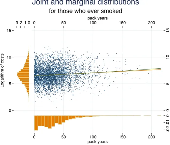
The idea of turning the axes of the figure into data can be taken a step further by showing the marginal distributions of y and x as histograms. This complements the scatter of points that show their joint distribution. At the same time both linear and quadratic fits of the data are added to the scatter plot to reflect the conditional relationship between y and x (see Figure 2.6).
Fig 2.6 Scatter plot and histograms combined
The Stata code required to do this is rather trickier in order to correctly rotate and align the three graphs that are combined in the final image:
clonevar y_s=lny clonevar x_s=treat
tw (scatter y_s x_s, msymbol(p)) (lfit y_s x_s)
(qfit y_s x_s)
if d==1,legend(off) yscale(alt noline) xscale(alt noline) xlabel(,grid gmax angle(horizontal))
ylabel( , angle(vertical)) saving(yt, replace)
0 5 10 15
L
o
g
a
ri
th
m
o
f
co
st
s
0 .1 .2 .3
0
5
1
0
1
5
0 50 100 150 200
pack years
0
.0
1
.0
2
0 50 100 150 200
pack years source: NMES 1987
quietly tw histogram y_s if d==1,
xsca(alt reverse noline) ysca(noline)
fxsize(20) horiz ylabel( , angle(horizontal)) xt(" ") saving(hy,replace)
quietly tw histogram x_s if d==1,
yscale(alt reverse noline) xsca(noline) ylabel(0(.01).02, nogrid) yt("")
xlabel(, grid gmax) fysize(20) saving(ht, replace)
graph combine hy.gph yt.gph ht.gph, hole(3) imargin(0 0 0 0) graphregion(margin(l=15 r=15)) note($note) title("Joint and marginal distributions") subtitle("for those who ever smoked") saving(scatter&margs, replace)
Note in particular how the x and y scales for the component graphics have to be reversed (reverse) and moved to the alternative side (alt) of the graphics from the default settings and how the axis lines
are removed (noline). The graphic is drawn for the sub-sample who
have ever smoked, reflected in the condition if d==1. The
command graph combine allows the three component graphics to
be spliced together and note how the hole(3) subcommand is used
to control their positioning by placing a space in the bottom left-hand corner.
Experimental research and statistical analysis by Cleveland and McGill (1984) has been highly influential and is cited by many recent authors (e.g., Cairo, 2012; Robbins, 2005; Yau, 2011). They demonstrated how there is a hierarchy in terms of the perception of visual cues and in how accurately people are able to read quantitative information from these cues. The hierarchy runs from the most accurate which is our ability to distinguish points along a common scale, or on different scales, then through differences in length, angles, direction, areas, volumes, shading/saturation, and finally colour/hue. The position of volume in this list is one reason that 3-D plots are inadvisable compared to simple 2-D plots.
Cairo (2013) and Nussbaumer Knaflic (2015) draw on further lessons from cognitive psychology and discuss the ways in which the gestalt principles of visual perception can be used to aid graphical design. These principles include:
Proximity:objects which appear close to each other are perceived as groups.
Similarity: visually identical objects are perceived as belonging to a group.
Connectedness: objects that are linked, for example by a line, are perceived as a group.
Closure: objects within crisp boundaries are perceived as belonging to a group.
Continuity: it iseasier to perceive shapes when contours are smooth and rounded.
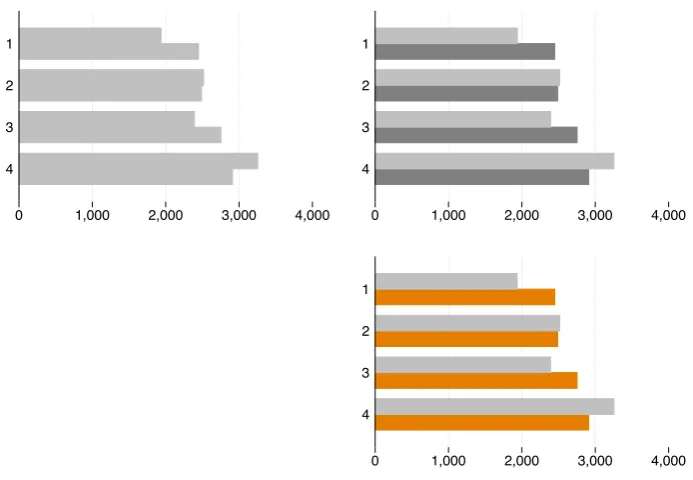
[image:20.595.127.474.452.692.2]As an illustration of some of these ideas consider the horizontal bar chart in Figure 2.7.
Fig 2.7 Using saturation and hue to suggest groups 0 1,000 2,000 3,000 4,000
4 3 2 1
0 1,000 2,000 3,000 4,000 4
3 2 1
0 1,000 2,000 3,000 4,000 4
3 2 1
The length of the bars represents average levels of medical costs and these are split between those who had never smoked and those who had ever smoked. So, despite the fact that there are no labels on the graphic, due to their proximity and the use of space to separate them, the pairs of bars labelled 1, 2, 3 and 4 are likely to be perceived as a group. These groups do in fact correspond to four levels of educational attainment. In the top left panel it is hard to distinguish the bars for smokers and non-smokers as they have the same shading and colour. The distinction becomes clearer in the other two panels that use differences in shading or in hue. Again there are no labels to make this explicit but the dark shaded bars in the top panel or the dark orange bars in the bottom panel will be perceived as a group. In this case the darker/orange bars represent the smokers within each level of education.
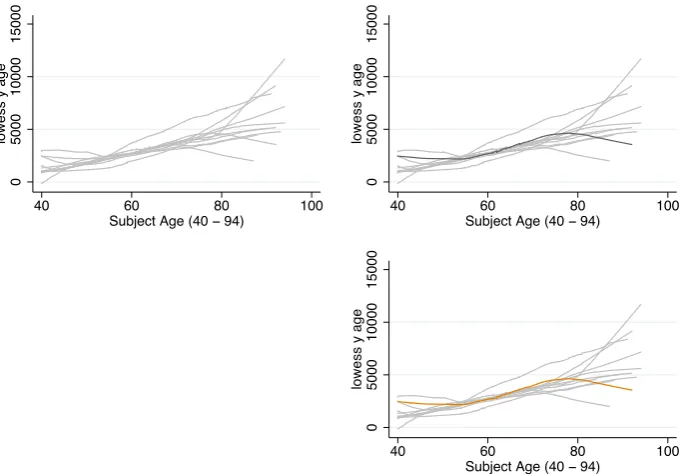
[image:21.595.130.471.436.673.2]Similarity and difference can be used to draw attention to particular features of a graphic and to highlight certain results. Figure 2.8 shows lowess fits of the relationship between medical costs and age for those aged over 40 for different sub-samples. The right-hand panels show how contrasts in saturation or hue can be used to highlight one particular line, such as the results for the full sample or for a particular group of interest.
Fig 2.8 Using saturation and hue to highlight
0
5
0
0
0
1
0
0
0
0
1
5
0
0
0
lo
w
e
ss
y
a
g
e
40 60 80 100
Subject Age (40 − 94)
0
5
0
0
0
1
0
0
0
0
1
5
0
0
0
lo
w
e
ss
y
a
g
e
40 60 80 100
Subject Age (40 − 94)
0
5
0
0
0
1
0
0
0
0
1
5
0
0
0
lo
w
e
ss
y
a
g
e
40 60 80 100
Subject Age (40 − 94)
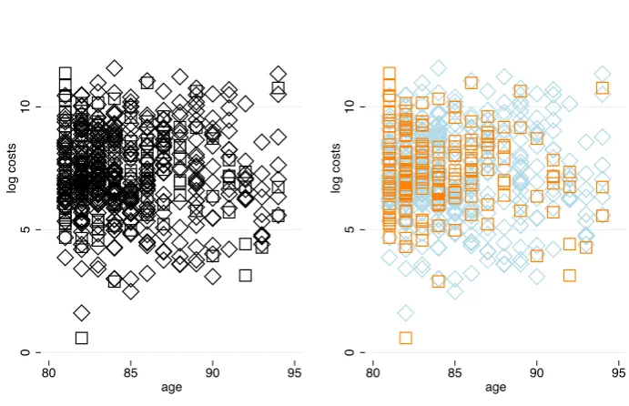
Figure 2.9 uses the idea that identical objects will be perceived as a group, here squares are used to denote smokers and diamonds are non-smokers in a scatter plot of the logarithm of medical costs against age for those aged 80 and over. The difference between the two groups is clearer to see when colour is added and the orange squares can be distinguished from the blue diamonds.
Fig 2.9 Using shape and hue to suggest groups
The code for Figure 2.9, which sets the shape, size and colour used for the data points, is:
tw (scatter lny $xc if d==0 & age>80, msize(vlarge) msymbol(Dh) mcolor(black) ysca(noline)
xsca(noline) legend(off) ytitle(log costs)) (scatter lny $xc if d==1 & age>80, msize(vlarge) msymbol(Sh) mcolor(black) ysca(noline)
xsca(noline) legend(off) ytitle(log costs) xtitle(age)), saving(sc1, replace)
tw (scatter lny $xc if d==0 & age>80, msize(vlarge) msymbol(Dh) mcolor(ltblue) ysca(noline)
xsca(noline) legend(off) ytitle(log costs))
(scatter lny $xc if d==1 & age>80, msize(vlarge) msymbol(Sh) mcolor(orange) ysca(noline)
xsca(noline) legend(off) ytitle(log costs)
0
5
1
0
1
5
lo
g
co
st
s
80 85 90 95
age
0
5
1
0
1
5
lo
g
co
st
s
80 85 90 95
age
xtitle(age)), saving(sc2, replace) graph combine sc1.gph sc2.gph, note($note)
The findings of Cleveland and McGill (1984) on how visual cues are perceived may create the impression that points along a common scale should always be preferred over the use of differences in saturation or hue. In fact, extracting precise quantitative comparisons is only one purpose of an effective graphic and very often making broad qualitative comparisons is important as well. The lesson of the preceding examples is that the use colour or shading often works best to create an immediate and bold impression of groups and proximity.
Camoes (2016) summarises the uses of colour in graphics as being to:
- Categorise.
- Group.
- Emphasize.
- Sequence.
- Diverge. - Alert.
A software package, such as Stata, will typically offer a palette of
Òbuilt inÓ colours such as the shade of dkorange used in the custom
scheme for this article. The available colours can be found under colorstyle. At a more fundamental level colour is typically defined and controlled using colour systems that can be used to mix your own colours. The RGB model defines colours in terms of their mix of red, green and blue. For example:
(0,0,0) - black (255,0,0) - red (0,255,0) - green (0,0,255) - blue (255,0,255) - magenta (255,255,255) - white
Camoes (2016) notes that when colours are ordered by hue there is an analogy with qualitative (ordinal or categorical) data. While when they are ordered by luminance there is an analogy with continuous quantitative variables. So, for example, hue can be used to create a Òdiverging scaleÓ that might be used to represent data from a Likert scale in a sequence such as red-orange-yellow-blue. This is typical of the heat map and tree map styles of graph. While Òcolour rampsÓ, created by selecting a hue and progressively changing the level of luminance, can capture the sense of continuous variation (if not the magnitudes). In Stata this can be done by taking a particular colorstyle and modifying its intensity, for
example, dkorange*.6. Or if an RGB value is used, 0 255 255*.8.
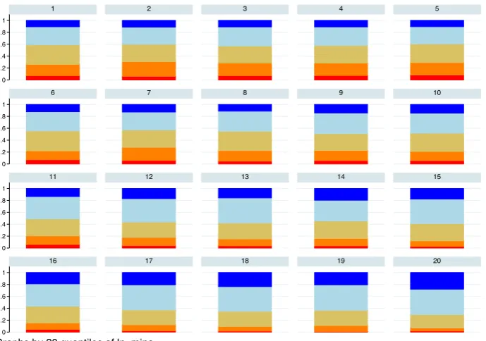
[image:24.595.128.473.427.669.2]Figure 2.10 uses a diverging scale to represent self-assessed health (SAH) data. SAH is an ordinal variable with responses ranging from poor, fair, good, very good, to excellent, This is represented by a scale that borrows the idea of a heat map and runs from a cool blue for excellent health to a hot red for poor health, The bar charts show the distribution of SAH over vigiciles of household income ranging from 1 which is the poorest group to 20 which is the richest. The greater concentration of poor and fair health among poorer households is clear.
Fig 2.10 Income gradients in SAH in UKHLS
0 .2 .4 .6 .8 1
0 .2 .4 .6 .8 1
0 .2 .4 .6 .8 1
0 .2 .4 .6 .8 1
1 2 3 4 5
6 7 8 9 10
11 12 13 14 15
16 17 18 19 20
Figure 2.11 shows the relationship between cholesterol, age, gender and income. It presents a set of smoothed lowess plots for the ratio of total to HDL cholesterol against age in years. A diverging scale of blue (ebblue) and dark orange (dkorange) is used to contrast results for men, in blue, and women, in orange. Within these a colour ramp distinguishes separate plots by deciles of household income, with lighter hues corresponding to lower incomes. The graphic reveals higher levels of the cholesterol ratio and a more pronounced hump shape in middle age for men as well as evidence of income gradients for both men and women.
Fig 2.11 Cholesterol ratio by age, gender and income in UKHLS
A colour wheel can be used as a guide to select the particular palette of colours to use in a graphic in order to have a pleasing and harmonious appearance and hence capture and retain the readerÕs attention. When a two-colour scheme is used these can be complementary and appear at 180o from each other on the colour wheel. Three-colour schemes include triadic harmony (120o from each other), split complementary, analogous colours (close together on the wheel), or warm and cool combinations. A four-colour scheme might be based on the rectangle rule (90o from each other).
2.5 3 3.5 4 4.5
lo
w
e
ss
tc_
h
d
l
a
g
e
_
n
u
rse
_
vi
si
t
20 40 60 80 100
age: @ UKHLS nurse visits sample