METHODS FOR ANALYSIS OF FUNCTIONALS ON
GAUSSIAN SELF SIMILAR PROCESSES
A Thesis submitted by
Hirdyesh Bhatia
For the award of
Doctor of Philosophy
Abstract
Many engineering and scientific applications necessitate the estimation of statistics of various functionals on stochastic processes. In Chapter 2, Norros et al’s Girsanov theorem for fBm is reviewed and extended to allow for non-unit volatility. We then prove that using method of images to solve the Fokker-Plank/Kolmogorov equation with a Dirac delta initial condition and a Dirichlet boundary condition to evaluate the first passage density, does not work in the case of fBm.
Chapter 3 provides generalisation of both the theorem of Ramer which finds a for-mula for the Radon-Nikodym derivative of a transformed Gaussian measure and of the Girsanov theorem. A
P
-measurable derivative of aP
-measurable function is defined and then shown to coincide with the stochastic derivative, under certain assumptions, which in turn coincides with the Malliavin derivative when both are defined. In Chap-ter 4consistent quasi-invariant stochastic flows are defined. When such a flow trans-forms a certain functional consistently a simple formula exists for the density of that functional. This is then used to derive the last exit distribution of Brownian motion.Thesis certification page
This Thesis is entirely the work of Hirdyesh Bhatia except where otherwise acknowl-edged. The work is original and has not previously been submitted for any other award, except where acknowledged.
Principal Supervisor: Ron Addie
Associate Supervisor: Yury Stepanyants
Acknowledgments
It is with immense gratitude that I acknowledge the support and help of my research supervisor associate professor Ron Addie, who has been my friend, guide and philoso-pher. This dissertation would also have remained a dream, had it not been for support of my wife, parents and friends. They always stood by me and dealt with all of my absence from many family occasions with a smile. I am also indebted to Professor Yury Stepanyants who reviewed several drafts of my solution attempts and provided valuable feedback on many problems which i encountered as part of this research. I would also like to offer my special thanks to Ilkka Norros, who provided invaluable feedback with this research project.
I am also grateful to Australian Commonwealth Government’s contribution through their Research Training Scheme (RTS) Fees Offset scheme, to help support this re-search. Thank you!
HIRDYESH
BHATIA
Contents
Abstract i
Acknowledgments iii
List of Figures v
Chapter 1 Introduction 1
1.1 Standard and Anomalous diffusion processes . . . 2
1.2 Fractional Brownian motion . . . 3
1.3 Functionals . . . 4
1.3.1 First Passage, Infimum and Supremum connections . . . 5
1.3.2 An example of Applications . . . 5
1.3.2.1 Applications of the supremum functional . . . 5
1.3.2.2 Applications of the first passage functional . . . 6
1.4 Fokker-Plank/Kolmogorov equations . . . 8
CONTENTS v
1.4.2 Boundary Conditions . . . 11
1.4.3 Fractional Brownian motion . . . 12
1.5 Derivatives associated with Stochastic processes . . . 13
1.5.1 Radon-Nikodym derivatives of transformations . . . 13
1.5.2 The Girsanov Theorem . . . 17
1.5.3 Derivatives on Abstract Wiener Space . . . 18
1.5.3.1 Gross-Sobolev derivative . . . 19
1.5.3.2 Stochastic derivative . . . 20
1.5.3.3 Malliavin derivative . . . 21
1.6 Fractional calculus on an interval . . . 23
1.7 Flows and probability theory . . . 24
1.8 Some known densities . . . 25
1.8.1 Supremum and Infimum Results . . . 26
Chapter 2 First Passage Problems 28 2.1 Pickands Constant . . . 29
2.2 Preliminary results . . . 30
2.3 Initial Boundary value problems for first-passage . . . 31
2.3.1 Stochastic processes in bounded domain . . . 31
CONTENTS vi
2.3.3 Failure of method of images for fBm . . . 32
Chapter 3 Radon-Nikodym derivatives associated with transformations 37 3.1 Abstract Wiener Space . . . 38
3.1.1 Radon-Nikodym Derivatives . . . 41
3.1.2 Paths . . . 41
3.1.3 Most likely functions . . . 45
3.2 Additive set functions and
P
-measurability . . . 473.2.1
P
-measurable functions . . . 493.2.2 The
P
-measurable Derivative . . . 573.2.3 The Radon-Nikodym Derivative . . . 61
3.2.4 Ramer’s theorem inH . . . 63
3.2.5 Girsanov Form . . . 66
3.2.6 Measurable extensions . . . 70
3.3 Example Applications . . . 72
3.3.1 A First Example . . . 73
3.3.2 A second example . . . 74
3.3.3 A Counter-example . . . 76
CONTENTS vii
4.1.1 Non-linear transformation of Gaussian measures . . . 79
4.1.2 The path spaces . . . 80
4.1.3 Definition . . . 80
4.2 The main theorem . . . 82
4.2.1 A Simple Example of a Flow . . . 83
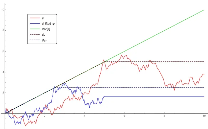
4.3 The last exit of Brownian motion . . . 84
4.3.1 A consistent quasi-invariant flow . . . 84
4.3.2 The Radon-Nikodym derivative ofλδ . . . 85
4.3.3 The last-exit density . . . 89
Chapter 5 Probability densities of functionals of fBm with drift 90 5.1 Supremum of fBm with drift . . . 90
5.1.1 The model and related work . . . 90
5.1.2 The mean, variance, third central moment and Skewness . . . 92
5.1.3 Simplifications of E[Q]and Var[Q]for certainH values . . . . 93
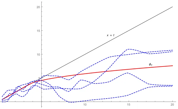
5.1.4 Consistency of the density under self similar transformation . 94 5.2 The Self Similarity PDEs . . . 95
5.2.1 Self Similarity PDE for supremum of fBm with drift . . . 95 5.2.2 Self Similarity PDE for First passage time of fBm with drift . 99
CONTENTS viii
List of Figures
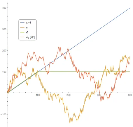
3.1 The most likely path passing through x=t att =4 and some random paths which are close to having this property. In this example,H=0.72. 45 3.2 A path and its transformation by the mapping (3.50) . . . 74 3.3 The transformationeλ
δapplied to a path causing a new last exit to
ap-pear (δ=0.5) . . . 77
Chapter 1
Introduction
The aim of this research is to develop methods for analysis of probability distribu-tions of the functionals on Gaussian Self similar processes amenable. However, for the reader’s convenience, in this chapter we review the main properties of various mathe-matical objects related to this research.
We begin by providing motivation behind the use of fractional Brownian motion and how it used for modeling Anomalous diffusion. The functionals being studied in this research are then defined and the reasons which motivate their study are provided. We then review the Fokker-Plank/Kolmogorov equations theory related to Markovian processes and how it is used to study the probability distribution of the first passage functional.
The development of measure theory by Lebesgue (Lebesgue 1904) enabled proba-bility theory to be given rigorous foundations, which was achieved by Kolmogorov (Kolmogorov 1950). Understanding probability as a measure has had a profound and ongoing influence on both theoretical and applied probability.
1.1 Standard and Anomalous diffusion processes 2
As the reproducing kernel Hilbert space associated with fBm considered as a vector space of functions (and not taking account of its Hilbert space structure and its norm) has a representation as the fractional spaceIH+
1 2
0+
L[0,T]
of certain class of functions, some standard results from fractional calculus are recalled to be used in the verification of a second generalisation of the Girsanov theorem for fBm later.
As part of this research, in Section 4.3 a quasi invariant flow with additional constraints is used to find a new proof of the probability distribution of the last exit of a Brownian motion process. We present a brief literature review on this subject next, which is followed by a review of the theory of probability densities of functionals on Brownian motion.
1.1
Standard and Anomalous diffusion processes
The concept of diffusion is widely used in physical sciences, economics and finance. However, in each case, the object (e.g., atom, price, etc.) that is undergoing diffusion is spreading out from a point or location at which there is a higher concentration of that object. The mathematical modeling of diffusion has a long history with many different formulations including, models based on conservation laws, random walks and central limit theorem, Brownian motion and stochastic differential equations, and models based on Chapman-Kolmogorov and Fokker-Planck equations. A fundamental result common to the different approaches is that the mean square displacement of a diffusing particle scales linearly with time. However there have been numerous exper-imental measurements in which the mean square displacement of diffusing particles scales as a non linear law in time.
Ben-1.2 Fractional Brownian motion 3
Avraham 1987) and fractional Brownian motion.
1.2
Fractional Brownian motion
The following definition is taken from (Lamperti 2012)
Definition 1.2.1. A stochastic process{X(t):t∈T}is defined as a collection of
ran-dom variables defined on a common probability space(Ω,
F
,P), whereΩis a samplespace,
F
is aσ-algebra, and P is a probability measure, and the random variables,indexed by some set T , all take values in the same mathematical space S, which must
be measurable with respect to someσ-algebraΣ.
Fractional Brownian motion was first introduced by Kolmogorov in 1940 in (Kol-mogorov 1940), within a Hilbert space framework, where it was called the Wiener Helix. It was further studied by Yaglom in (Yaglom 1955). The name fractional Brow-nian motion has been coined by Mandelbrot and Van Ness, who in 1968 provided in (Mandelbrot and Ness 1968) a stochastic integral representation of this process in terms of a standard Brownian motion. The following definition of fractional Brownian motion can be found in (Biagini et al. 2008a).
Definition 1.2.2. Let Hurst index H be a constant belonging to (0,1). A standard
fractional Brownian motion (fBm) BH(t)t≥0is a continuous and centered Gaussian
process, which starts at zero, has expectation zero for all t∈[0,T]with the covariance
function
EBH(t)BH(s)= 1
2 t
2H+s2H− |t−s|2H .
ForH= 12, fBm is then a standard Brownian motion process. By Definition 1.2.2 we obtain that a standard (fBm) BH(t)t≥0process has the following properties:
• BH(0) =0 andEBH(t)=0 ∀ t ≥0.
1.3 Functionals 4
• BH is a Gaussian process andE
h
BH(t)2
i
=t2H,t ≥0 ∀ H ∈(0,1).
The existence of fBm follows from the general existence theorem of centered Gaus-sian processes with given covariance functions (Rogers and Williams 1994, Nourdin 2012). It is also noteworthy that the situation with continuity of fBm trajectories is more involved, as in we can consider a continuous modification of fBm which ex-ists according to Kolmogorov continuity theorem which guarantees that a stochastic process that satisfies certain constraints on the moments of its increments will have a continuous version (Stroock and Varadhan 2007).
1.3
Functionals
The term functional refers to a real-valued function defined on vector space. When the paths of a stochastic process are used to model processes of practical importance, functionals will often represent quantities of economic or social interest, such as costs, resource consumption, service delays, and so on. Therefore it is of great interest to be able to determine the probability distribution of functionals. Currently there is no general method for tackling the problem of determining the distribution of a given functional defined on an abstract Wiener space.
A large class of functionals is defined in terms of aboundarywhich takes the same gen-eral form as a path, i.e. it is a real-valued function of time. Given a specific boundary, e.g. b(t), thefirst-passagefunctional before timeT >0 is defined as:
Definition 1.3.1.
Tb(ψ)=. inf[{t:(ψ(t)<b(t)∧b(0)<ψ(0))∨(ψ(t)>b(t)∧b(0)>ψ(0))} ∪ {T}].
depending on the initial condition under which the stochastic process started. The past supremum and the past infimum will denoted as supt≤Tψt and inft≤Tψt. These
1.3 Functionals 5
Definition 1.3.2.
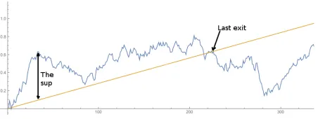
τb(ψ)=. inf[{sup{t:ψ(t)≥b(t)}} ∪ {T}].
The methods of this research are, in principle, applicable to all of them. We focus especially, however, on the first passage, supremum and the last-exit functionals, where the boundary is linear.
1.3.1
First Passage, Infimum and Supremum connections
LetTbbe the first time that the processψ(t)touches the barrierb, such thatψ(0)>b(0)
i.e. the first passage time to a lower barrier. The distributions of the first passage time and the minimum are strongly connected, indeed the event{Tb>T}is the same as the event{inft≤Tψ(t)>b(t)}. We can thus write down the distribution ofTb
P
inf
t≤T[ψ(t)−b(t)]≤0
=P(Tb≤T). (1.1) Similarly the law of the past supremum supt≤Tψ(t)of a continuous stochastic process
before a deterministic timeT >0 also presents some major interest in stochastic mod-eling, such as queuing and risk theories, as it is related to the law of the first passage timeTbabove any levelbwhenb(0)>ψ(0), through the relation
P
sup
t≤T
[ψ(t)−b(t)]≥0
=P(Tb≤T). (1.2)
1.3.2
An example of Applications
1.3 Functionals 6
its accuracy has been validated by various publications including (Norros 1995, Chen et al. 2013). Although a queue fed by fBm input has been considered as a funda-mentally important model for Internet queueing performance analysis (Norros 1995, W. Willinger and Wilson 1997, Dijkerman and Mazumdar 1994, Hüsler and Piterbarg 1999, Duffield and O’Connell 1995, Chen et al. 2013, 2015), no explicit accurate re-sults for the mean, variance, third central moment and skewness for the occupancy,Q, of an fBm queue, are available.
1.3.2.1 Applications of the supremum functional
LetX(t)denote an arithmetic fractional Brownian process with driftµ, with SDE dX(t) =µdt+σdBH(t), X(0) =0
where BH is an fBm with H ∈[0,1]. There are various motivations for studying the probability distribution of supt∈[0,T]X(t). Fractional Brownian motion has been widely accepted as an accurate model of Internet traffic in parts of networks where there is sig-nificant aggregation (Leland et al. 1994, Norros 1995, W. Willinger and Wilson 1997, Taqqu et al. 1997). Other applications include studying pursuit problems (Bramson and Griffeath 1991, Li and Shao 2001), in study of extremes and level sets (Azaïs and Wschebor 2009). Hüsler and Piterbarg (Hüsler and Piterbarg 1999, Theorem 1, Equation (9)) (withα=2H,β=1) have shown that
P
sup
t>0
X(t)>x
∼Cx2H
2−3H+1
H e
−x2−2H(1−H)2H−2|µ|2H
2H2Hσ2
(1.3) for someC>0 (which is given explicitly in (Hüsler and Piterbarg 1999)), in the sense that the ratio of the two sides of (1.3) tends to 1 asx→∞. A variety of results related to
tail asymptotics, extreme value theorems, laws of iterated logarithm etc are related to a set of certain constants known asPickands’ constants(Pickands 1969b,a). In particular, the formula for C given in (Hüsler and Piterbarg 1999) is expressed in terms of a Pickands’ constant.
According to (Mandjes 2007, Proposition 5.6.2), which is credited to be from (Debicki and Rolski 1999, Theorem 4.3) ifQdenotes the stationary contents of an fBm queue,
P(Q>x)
x2H−3+1/Hexp−1 2
x
1−H
2−2H µ H
2H→
α(H)
√
1.3 Functionals 7
asx→∞, in which
α(H) =
H
2H√
π
2(1−H)/2H√H
H µ(1−H)
H−1
1 1−H
(2−H)/H
and
β(H) =
µ(1−H)
H
H
1 1−H
where
H
x denotes the Pickands’ constant. Even in the case of µ=0, only boundsare known, to the best of our knowledge, for the tail probability of the supremum of fractional Brownian motion (Molchan 1999, Aurzada et al. 2011).
1.3.2.2 Applications of the first passage functional
There are also several other motivation for the study of the first passage functional other than its own importance, such as its relation to Burgers equation with random initial data (She et al. 1992, Bertoin 1998). Other applications include studying pursuit problems (Bramson and Griffeath 1991, Li and Shao 2001), in study of extremes and level sets (Azaïs and Wschebor 2009). Also in the field of Gaussian processes a variety of results related to tail asymptotics, extreme value theorems, laws of iterated logarithm etc are related to a set of certain constants known as Pickands’ constants(Qualls and Watanabe 1972, De¸bicki 2002, 2006, De¸bicki and Kisowski 2008, Arendarczyk and De¸bicki 2012, Albin 1994, Darling 1983).
Unfortunately little is known about the first passage probability of a fractional Brow-nian motion process. Martingale methods and Fokker-Plank boundary value problem approaches do not appear to have been successful in the caseH 6=0.5 so far.
1.3 Functionals 8
The first passage time density of fractional Brownian motion confined to a two-dimensional open wedge domain with absorbing boundaries has also been shown to satisfy
PΩ(t)≈t
−1+π(2H2Ω−2)
in the limit ast →∞, whereΩis the wedge angle, in (Jeon et al. 2011). Prakasa Rao
(Rao 2013) has obtain some maximal inequalities for a centered fractional Brownian motion with H∈ 12,1 and with a polynomial drift g(·)by studying the asymptotic behaviour of the tail distribution function
P
sup
0<t<T
BHt +g(t)>a
asT →∞for fixedaand asa→∞for fixedT. Molchan (Molchan 1999), has shown TH−1exph−βplogT
i
≤P(τ1>T)≤TH−1exp
h
βplogT
i
for some constant βasT goes to infinity. These bounds have been improved by Au-rzada (AuAu-rzada et al. 2011) to
TH−1(logT)−α1 ≤
P(τ1>T)≤TH−1(logT)α2 (1.4)
for some constants α1 > 21H and α2 > H2 −1, for large enough T. In the physics
literature, these results are often used in the sense ≈TH−1, disregarding the other factors.
For further background information and links to existing literature, we refer the reader to (Li et al. 2004).
1.4 Fokker-Plank/Kolmogorov equations 9
1.4
Fokker-Plank/Kolmogorov equations
The theory of Fokker-Plank/Kolmogorov equations, which are second order elliptic and parabolic equations for measures, goes back to Kolmogorov’s works (Kolmogoroff 1931) along with a number of earlier works in the physics literature by Fokker, Smolu-chowski, Planck and Chapman (Fokker 1914, Planck 1917). In the recent years several important monographs have also appeared (Bogachev et al. 2015, Risken 1996). One of the main objects here is the elliptic operator of the form
LA,bf =Tr AD2f+hb,∇fi, f ∈C0∞(Ω),
whereA= ai jis a mapping on a domainΩ⊂Rdwith values in the space of
nonnega-tive symmetric linear operators onRdandb= (bi)is a vector field onΩ. In coordinate
form,LA,bis given by the expression LA,bf =
d
∑
i,j=1
ai j∂xi∂xjf +
d
∑
i=1
bi∂xif.
From this operator we can define the adjointLA,b∗via the duality relation
Z
Ω
LA,bf
dµ=
Z
Ω
f d LA,b∗µ
∀f ∈C0∞(Ω),
andµ∈M Rd, the space of locally finite (possibly signed) Borel measures. The weak elliptic equation is associated with operatorLA,bas
LA,b∗µ=0, (1.5)
for Borel measures onΩ, furthermore we sayµsolves (1.5) if
Z
Ω
LA,bfdµ=0 ∀f ∈C0∞(
Ω), (1.6)
where we assume thatbi,ai j ∈Lloc1(µ), the class of locally integrable functions. It is noteworthy that this is the same as saying that (1.5) holds in the sense of distributions, where we recall that anyµ∈M Rdgives rise to a distribution in the natural way. Similarly, one can consider parabolic operators and parabolic Fokker-Planck Kolmogorov equations for measures onΩ×(0,T)of the type
1.4 Fokker-Plank/Kolmogorov equations 10
also in the sense of distributions (withA,bpossibly time-dependent). Hence, the study of these equations reduces to studying partial differential equations in the distributional setting, as shown in (Evans 2010, Gilbarg and Trudinger 2015, Friedman 2008, Re-nardy and Rogers 2006). However it is crucial that a priori Fokker-Planck-Kolmogorov equations are equations for measures, not for rough distributions (Bogachev et al. 2015). This becomes relevant when the coefficients are singular or degenerate and, in particular, in the infinite-dimensional case, where no Lebesgue measure exists. The theory of these equations for measures is now a rapidly growing area with connections to many other areas of mathematics such as real analysis, partial differential equations and stochastic analysis.
1.4.1
Probabilistic Motivation
For exposition of the semi-group of operators generated by the transition function of a Markov process, we recommend the reader to (Kallenberg 2006, Revuz and Yor 2013). For further details concerning the semi-group theory from a more functional analysis point of view, please see (Phillips and Hille 1957, Yosida 1995). Knowledge of the infinitesimal generator enables one to derive important characteristics of the initial process; the classification of Markov processes amounts to the description of their corresponding infinitesimal generators (Sarymsakov 1954, Gikhman and Skorokhod 2015). For semi-groups of transformations associated to parabolic partial differential equations, see (Feller 1952).
Suppose that ξ= (ξ(x,t))t≥0 is a diffusion process inRd governed by the stochastic
differential equation
dξ(x,t) =b(ξ(x,t))dt+σ(ξ(x,t))dWt, ξ0=x0. (1.8)
The generator of the transition semigroup{Tt}t≥0has the formLA,b, whereA=σσ∗/2.
The matrix A in the operator LA,b is known as the diffusion matrix or diffusion co-efficient and the vector field b is called the drift coefficient or just drift. Denote by P(x,t) (B) the probability that ξ moves from point x ∈Rd to a measurable set
B∈B Rd
(the Borel measurable sets in Rd) in time t ≥0. Hence, P(x,t) (·) is a
probability measure on Rd,Band(x,t)7→P(x,t) (·)is the so-called transition
1.4 Fokker-Plank/Kolmogorov equations 11
equation (1.7)(Friedman 2012). If the transition function satisfies certain locality con-ditions, then we sayξis a Markovian diffusion, more details are presented in (Øksendal
2003, Stroock 2008). A probability measureµis called invariant (Bogachev et al. 2001, Von Neumann 1941) for{Tt}t≥0if the following identity holds:
Z
Rd
Ttfdµ=
Z
Rd
fdµ ∀f ∈Cb
Rd
. (1.9)
Any invariant probability measure µofξ(if such exists) satisfies (1.5). Measures
sat-isfying (1.5) are called infinitesimally invariant, as this equation has deep connections with invariance with respect to the corresponding semigroups(Bogachev et al. 2015). Also, if there is an invariant probability measureµ, then{Tt}t≥0extends toL1(µ)and is strongly continuous. Denoting L to be the corresponding generator with domain D(L). Then (1.9) is equivalent to the equality
Z
Rd
L fdµ=0 ∀f ∈D(L).
Under some reasonable assumptions onAandb, the generator of the semigroup asso-ciated with the diffusion governed by the indicated stochastic equation coincides with LA,bonC∞
0 Rd
, but the invariance of the measure in the sense of (1.9) is not the same as (1.6), and the class C0∞
Rd may be much smaller than D(L) (Bogachev et al.
2015, Stroock and Varadhan 2007).
A diffusion SDE, can be used to define a deterministic function of space and time in two fundamentally different ways. First by considering the expected value of some function, as a function of the initial position and time. Secondly by considering the probability of being in a certain state at a given time, given the knowledge of the initial state and time (Øksendal 2003). Thus when studying the first scenario, one explores the mathematical ideas of the backward Kolmogorov equation and the Feynman-Kac formula. When studying the latter viewpoint, which is in fact dual to the first view-point, the evolving probability density solves a different PDE, the forward Kolmogorov equation, which is actually the adjoint of the backward Kolmogorov equation.
1.4 Fokker-Plank/Kolmogorov equations 12
1.4.2
Boundary Conditions
It is of interest to consider how and when a diffusion process crosses a barrier. Proba-bilistically, thinking about barriers means considering exit times. On the PDE side this leads us to consider boundary value problems for the backward and forward Fokker-Plank/Kolmogorov equations.
We now briefly summarize some of the common types of boundary conditions for the Fokker-Plank/Kolmogorov equations. Let us denote a Brownian motion beginning at x0.
dXt =dWt, X0=x0.
We know that the transition density p(x,t) satisfies the Fokker-Plank/Kolmogorov equation
−∂t+
1 2∂xx
2
p=0.
1. Natural boundary conditions: This is the condition that p(x,t)7→0 asx7→∞or
x7→ −∞. With the decay to zero being sufficiently fast to ensure the
normaliza-tion integral is
Z ∞
−∞
P(x,t)dx=1.
2. Absorbing boundary conditions: Now, suppose that we restrict the processXt to
a region [L,U]. We say Xt has an absorbing boundary condition atL, if, when
Xt hitsL, it stays there forever, which is modeled using the Dirichlet boundary
condition p(L,t) =0.
In case of processes associated with diffusion, absorbing boundary conditions are used to study first passage, supremum and infimum of probability densities corresponding to these processes.
3. Reflecting boundary conditions: Likewise, we say thatXthas a reflecting
bound-ary condition atL, if, whenXt hitsL, it is instantaneously reflected back into the
1.4 Fokker-Plank/Kolmogorov equations 13
1.4.3
Fractional Brownian motion
The Fokker-Plank/Kolmogorov equations are now well known for Fractional Brownian motion dependent processes as shown by subsequent lemma. Although the traditional techniques associated with studying first passage time density via the initial boundary value problems for Markovian processes are not applicable, as is shown in chapter 2. This is, due to the non-Markovian nature of the underlying processes.
The derivation of the Kolmogorov Forward Equation formula for fractional Brownian motion can be found in (Zeng et al. 2012). It should be noted this result was provided without any restrictions on the range of Hurst parameter H. Even though the original proof relies on fractional Itô formula proven for H ≥ 12 in (Duncan et al. 2000), the result has since been extended by modifying the fractional white noise approach (Hu and Øksendal 2003) to cover the range 0<H<1 in (Bender 2003). Similar equations have also been considered in (Baudoin and Coutin 2007, Hahn and Umarov 2011).
Lemma 1.4.1. (Kolmogorov Forward Equation formula for fBm). The Kolmogorov Forward Equation, also known as the Fokker-Plank equation associated with a
nonlin-ear fractional Brownian motion driven SDE of the form
dX(t) = f(X(t),t)dt+g(X(t),t)dBH(t) (1.10) where f(x(t),t)and g(x(t),t)are real-valued functions, not equal to0possessing the
indicated derivatives and BH(t)is a standard fBm with Hurst parameter H is
∂p(x,t)
∂t = −
∂(f(x(t),t)p(x,t)) ∂x
+ ∂
2 g(x(t),t)p(x,t)Rt
0g(x(s),s)φ(s,t)ds
∂x2 (1.11)
where
φ(s,t) =H(2H−1)|s−t|2H−2.
1.5 Derivatives associated with Stochastic processes 14
1.5
Derivatives associated with Stochastic processes
1.5.1
Radon-Nikodym derivatives of transformations
In the theory of stochastic processes, the influence of measure theory can be seen in the use of the term random function, instead of stochastic process, as in the books (Yaglom 2004, Lifshits 1995), for example. The concept that the study of stochastic processes is “really” the study of measures on spaces of functions entails difficulties as well as opportunities. In particular, it can be shown (Kuo 1975) that there is no rotationally or translationally invariant measure with bounded values on bounded sets, and positive values on open sets, on any infinite dimensional normed vector space, and hence the concept of probability density is no longer applicable. This challenge is potentially addressed by adopting Gaussian measures as the “standard measure” on function spaces.
The Cameron-Martin theorem(Cameron and Martin 1944) provides a partial substitute for the concept of a density in that it provides a “likelihood ratio” between two differ-ent Gaussian measures which differ by a shift from the Cameron-Martin space (also termed the space of measurable shifts), which is the space of vectors, a shift by which gives rise to a well-defined non-zero Radon-Nikodym derivative.
This result was extended by Girsanov(Girsanov 1960) to enable comparison of ar-bitrary Ito measures, i.e. measures constructed by a stochastic differential equation driven by Brownian motion. Extensions of the Girsanov theorem to processes defined by stochastic differential equations based on fractional Brownian motion, have also been developed in (Norros et al. 1999, Decreusefond 2000, 2003, Mishura 2008, Bi-agini et al. 2008b).
1.5 Derivatives associated with Stochastic processes 15
same, at this point. However, since the Radon-Nikodym derivative incorporates in an appropriate way the dilation or concentration effected by the transformation at each location, the Radon-Nikodym derivative can’t be isolated from the choice of transfor-mation linking the two measures.
A different extension of the Cameron-Martin theorem, to the situation where the trans-formation between measures is affine, was considered in (Segal 1958) and (Feldman 1958), and to the general nonlinear case in (Ramer 1974) and (Cruzeiro 1983b). The resulting formula in the first three cases takes the form of a product of two terms, one basically the same as the Cameron-Martin formula, and the other term is effectively the Jacobian of the nonlinear transformation.
Since a Jacobian is defined in terms of the derivative of the transformation (in this case the Fréchet derivative is appropriate), Ramer observed that the result can still hold when the traditional definition of Jacobian fails. He replaced the Jacobian by an expression partially induced, by continuity, from the action of the mapping on the Cameron-Martin space of the measure.
Even with this relaxation in the definition of the Jacobian, it appears to be very difficult to find non-trivial examples where Ramer’s formula for the Radon-Nikodym derivative can be evaluated, so it is appropriate to consider additional, or alternative ways in which the definition of Jacobian, or derivative of a transformation, can be generalised and made easier to apply.
A Malliavin derivative of a transformation between measure spaces may exist when the traditional Frechét derivative does not. One of the objectives of the Malliavin derivative is to evaluate a derivative which can’t be evaluated by conventional means. Note: it is not the derivative of a path that concerns us here, but the derivative of a transformation of paths. The conventional derivative to be used here is the Frechét derivative. But the limits in the Frechét derivative either can’t be evaluated, or at least are very difficult to evaluate.
1.5 Derivatives associated with Stochastic processes 16
The
P
-measurable derivative introduced in Subsection 3.2.2 takes exactly the same form as a Frechét derivative, namely it is still a linear operator on the space of paths, but the limits required in its definition are weaker than conventional limits. This is achieved by using a limit inP
-measure in the definition of the derivative.The concept of limits in
P
-measure, whereP
is some measure or finitely additive set function, has a long history, going back to the start of measure theory, and continuing to this day. In this researchP
will always refer to thestandard Gauss measure(Kuo 1975), which, despite the name, is a finitely additive set function, and not, in general, a measure. The key highlights of the theory of finitely additive set functions (P
say), theP
-measurable functions, and integration ofP
-measurable functions with respect to the measureP
, including the appropriate Radon-Nikodym theorem, are presented in (Dunford and Schwartz 1957).Once the step of using
P
-measurable functions uniformly in the theory is taken, the Ramer theorem takes exactly the same form as the corresponding Jacobian theorem which would apply if the spaces were all finite-dimensional. The proof of this theorem is also dramatically simpler than in (Ramer 1974).In (Cruzeiro 1983b), the context was not Gaussian measure spaces in general but the specific case of the space C[0,1] with the Wiener measure. In place of a non-linear transformation, Cruzeiro considers a vector field, which defines a flow on the Wiener space. The Radon-Nikodym derivative is now expressed more directly as an integral involving the divergence of the vector field.
In the present research not only the Jacobian, but the formula for the Radon-Nikodym derivative itself is found on the Cameron-Martin space, first, and then the result on the path space is induced by continuity from its value on Cameron-Martin space. This allows us to avoid highly restrictive conditions on the class of non-linear mappings to which the theory can apply.
1.5 Derivatives associated with Stochastic processes 17
The idea that it may be more useful to obtain the Radon-Nikodykm derivative on the
Cameron-Martin space also motivates the authors of (Bagchi and Mazumdar 1993),
where the application in mind is to generalise the concept of stochastic process (or random function) to include white noise, which is not a well-defined random function in the conventional sense. The role of measures, in the Cameron-Martin space, is taken
by finitely additive set functions, and while there is no probability measure for white
noise on the whole path space, the identity mapping can be interpreted as a white noise random function defined on the Cameron-Martin space.
There is scope for a theorem which generalises both the Girsanov theorem and the Ramer theorem. We present such a generalisation of the Girsanov theorem for fBm in this research, which is not limited to changes in linear drift only in theorem 3.2.3. Although our goal is primarily to make the Ramer theorem easier to apply, by identi-fying a different type of regularity condition on the function, f, which makes it easy to identify functions to which it can be applied, and easy to evaluate the Radon-Nikodym derivative formula. The key new regularity condition on f which is adopted is
P
-measurability.A simple form of the Ramer theorem is shown to apply to the transformation applying on a Hilbert space equipped with an additive set function. Except for needing the theory of
P
-measurable functions, the proof of this result is quite simple.Also, it is shown that a Radon-Nikodym derivative between finitely additive measures on the Cameron-Martin space of a Gaussian measure can be uniquely extended to the original space and provides a Radon-Nikodym derivative there. Using this exten-sion theorem, the Ramer theorem onHcan be readily used to derive Radon-Nikodym derivatives between a Gaussian measure and its transformation by a
P
-measurable function between spaces.1.5 Derivatives associated with Stochastic processes 18
1.5.2
The Girsanov Theorem
Although more general versions of Girsanov formula for fractional Brownian motion are known (Decreusefond et al. 1999, Mishura and Valkeila 2001), in this research we consider Norros et al’s version of Girsanov formula for fractional Brownian motion. A proof of the following Girsanov formula for fractional Brownian motion can be found in (Norros et al. 1999), where the term the fundamental martingale is also coined for the processMt.
Proposition 1.5.1. (The Girsanov formula for fBm). Let BH(t)denote fractional Brow-nian motion with mean0and variance t2H, for all H∈(0,1)defined on(Ω,
F
,P). Leta be a scalar. Define a new probability measureQon(Ω,
F
)via the Radon Nikodymderivative with respect toP
dQ
dP =exp
µMT−1
2µ
2hM
,MiT
(1.12) where
MT =
1
2HΓ 32−HΓ H+12
Z T
0
(s(T−s))12−HdB
sH. (1.13)
The process MT is a martingale with independent increments, zero mean and variance
function c2T2−2H where
c=
s
Γ 32−H
2H(2−2H)Γ H+12Γ(2−2H)
. (1.14)
Then the process defined, for all t ∈[0,T], by BH(t) +µt is the standardQ-fractional
Brownian motion on [0,T]. In other words, under probability measure Q, BH(t)
re-stricted to t ∈[0,T] is distributed as an arithmetic fractional Brownian motion with
drift µ.
It’s noteworthy that using the variance ofMt, (1.12) can also be re-written as
dQ dP =exp
µMT−1
2µ
2c2T2−2H
. (1.15)
1.5 Derivatives associated with Stochastic processes 19
Corollary 1.5.1. Let X(t) =bBH(t)be an arithmetic fractional Brownian motion with
volatility b, for all H ∈(0,1) defined on (Ω,
F
,P). Let a be a scalar. Define a newprobability measureQon(Ω,
F
)via the Radon Nikodym derivative with respect toPdQ
dP =exp
a
bMT−
1 2
a2 b2c
2T2−2H
. (1.16)
Then the process defined, for all t ∈[0,T], by Z(t) =X(t) +at is an arithmetic Q
-fractional Brownian motion process on [0,T]with volatility b. In other words, under
probability measure Q, X(t) restricted to t ∈[0,T] is distributed as an arithmetic
fractional Brownian motion with drift a and volatility b.
Proof. The change of measure (1.15) turns the process dBH(t)into the process dBH(t)+
µdt. Therefore, if we use this weight function, on the processX(t)we get dX(t) =
b dBH(t) +µdt. This becomes the processZ(t)if
µ= a
b.
Therefore, the likelihood ratio betweenX(t)andZ(t)is as claimed.
1.5.3
Derivatives on Abstract Wiener Space
In measure theory, abstract Wiener space is used to construct a strictly positive and locally finite measure on an infinite-dimensional vector space. A more formal presen-tation of this concept can be found in section 3.1. The following two definitions and the subsequent proposition can be found in (Di Nunno et al. 2009). LetX be a Banach space that is, a complete, normed vector space over R. The set of all bounded linear functionals is called the dual ofX and is denoted byX∗. LetU be an open subset of a Banach spaceX and let f be a function fromU intoR.
Definition 1.5.1. We say that f has a directional derivative (or Gateaux derivative) Dyf(x)at x∈U in the direction y∈X if
Dyf(x):= d
dε[f(x+εy)]ε=0∈R (1.17)
1.5 Derivatives associated with Stochastic processes 20
Definition 1.5.2. We say that f is Fréchet-differentiable at x ∈U , if there exists a
bounded linear map A:X 7→R, that is, A∈X∗, such that
lim
h→0;h∈X
|f(x+h)−f(x)−A(h)|
khk =0. (1.18)
We write
f0(x) =A∈X∗, (1.19)
for the Fréchet derivative of f at x.
Proposition 1.5.2. If f is Fréchet differentiable at x∈U⊂X , then f has a directional
derivative at x in all directions y∈X and
Dyf(x) =hf0(x),yi ∈R. (1.20)
Conversely, if f has a directional derivative at all x∈U in all directions y∈X and the
linear map
y7→Dyf(x), y∈X (1.21)
is continuous∀x∈U , then there exists an element∇f(x)in X∗such that
Dyf(x) =h∇f(x),yi. (1.22)
If this map x7→∇f(x)∈X∗is continuous on U , then f is Fréchet differentiable and
f0(x) =∇f(x). (1.23)
1.5.3.1 Gross-Sobolev derivative
LetW =C0([0,1],R)be the classical Wiener space equipped with Wiener measureµ.
1.5 Derivatives associated with Stochastic processes 21
is necessary: ifF,G∈Lp(µ), and ifF =G µ- a.s., it is natural to ask that their deriva-tives are also equal a.s. For this, the only way is to choose yin a specific subspace of W, namely the Cameron-Martin spaceH:
H ={h:[0,1]7→R/h(t) =
Z t 0
ˆ
h(s)ds,|h|H2=
Z 1
0
|hˆ(s)|2ds}. (1.24) We now briefly sketch the construction of this derivative, for more details please see (Üstünel 2010). Let S(Rn) denote the space of infinitely differentiable, rapidly de-creasing functions on Rn. If F :W 7→R is a function of the following type (called cylindrical ):
F(x) = f(Wt1(x),· · ·,Wtn(x)), f ∈S(Rn), (1.25) we define, fory∈H, the directional derivative as
DyF(x) =
d
dε[F(x+εy)]ε=0. (1.26)
SinceWt(x+y) =Wt(x) +y(t), we obtain
DyF(x) =
n
∑
i=1
∂if(Wt1(x),· · ·,Wtn(x))y(ti), (1.27) in particular
DyWt(x) =y(t) =
Z t 0
ˆ
h(s)ds=
Z t 0
1[0,t](s)hˆ(s)ds. (1.28) If we denote byUtthe element ofHdefined asUt(s) =Rs
01[0,t](r)dr, we haveDyWt(x) =
hUt,yiH. Looking at the linear map y7→DyF(x) we see that it defines a random
el-ement with values in H∗, since we have identified H with H∗, D(F) is anH-valued random variable. It can be shown that Dis a closable operator on anyLp(µ) (p>1)
and it can be extended to larger classes of Wiener functionals than the cylindrical ones, as defined below.
Definition 1.5.3. F ∈Domp(D) if and only if there exists a sequence (Fn;n∈N) of
cylindrical functions such that Fn7→F in Lp(µ) and (DFn) is Cauchy in Lp(µ,H).
Then, for any F∈Domp(D), we define
D(F) = lim
n→∞
D(Fn). (1.29)
1.5 Derivatives associated with Stochastic processes 22
1.5.3.2 Stochastic derivative
The definitions and theory in the current and next subsection are much more compre-hensively presented in (Di Nunno et al. 2009).
Definition 1.5.4. Let F :W 7→R be a random variable, choose g ∈L2([0,T]), and consider
γ(t) =
Z t 0
g(s)ds∈W. (1.30)
Then we can define the directional derivative ofF similar to (1.26).
Definition 1.5.5. Assume that F :W 7→Rhas a directional derivative in all directions
γof the formγ∈H in the strong sense, that is,
DγF(ω):=lim ε→0
F(ω+εγ)−F(ω)
ε (1.31)
exists in L2(P). Assume in addition that there existsψ(t,ω)∈L2(P×λ)such that
DγF(ω) =
Z T
0
ψ(t,ω)g(t)dt, ∀γ∈H. (1.32)
Then we say that F is differentiable and we set
DtF(ω):=ψ(t,ω). (1.33)
We call D.F ∈L2(P×λ)the stochastic derivative of F. The set of all differentiable
random variables is denoted buD1,2.
1.5.3.3 Malliavin derivative
1.5 Derivatives associated with Stochastic processes 23
This new approach proved to be extremely successful and soon a number of authors studied variants and simplifications of the original proof (Bismut 1981b,c, Kusuoka and Stroock 1984, 1985, Norris 1986).
Even now, more than three decades after Malliavin’s original work, his techniques prove to be sufficiently flexible to obtain related results for a number of extensions of the original problem, including for example SDEs with jumps (Takeuchi 2002, Ishikawa and Kunita 2006, Cass 2009, Takeuchi 2010), infinite-dimensional systems(Ocone 1988, Baudoin et al. 2005, Mattingly and Pardoux 2006), and SDEs driven by Gaus-sian processes other than Brownian motion(Baudoin and Hairer 2007, Cass and Friz 2010, Hairer et al. 2011, Cass et al. 2015).
LetPdenote the family of all random variablesF:Ω7→R of the form
F =φ(θ1,· · ·,θn), (1.34)
whereφ(x1,· · ·,xn) =∑αaαxα, withxα =x1α· · ·xnα andα= (α1,· · ·,αn),is a
poly-nomial and θi=R0T fi(t)dW(t) for some fi ∈L2([0,T]),i=1,· · ·,n. Such random
variables are called Wiener polynomials. It should be noted thatPis dense inL2(P).
LetF=φ(θ1,· · ·,θn)∈P. ThenF∈D1,2and
DtF=
n
∑
i=1
∂φ ∂θi
(θ1,· · ·,θn).fi(t). (1.35)
We now introduce the norm|| · ||1,2onD1,2:
||F||21,2:=||F||2L2(P)+||DtF||2L2(P×λ), F ∈D1,2. (1.36)
Unfortunately, as it is not clear if D1,2 is closed under this norm, hence one works
instead with the following family.
Definition 1.5.6. We defineD1,2 to be the closure of the familyPwith respect to the
norm|| · ||1,2.
ThusD1,2consists of allF∈L2(P)such that there existsFn∈Pwith the property that
Fn→F in L2(P) asn→∞ and{DtFn}∞n=1 is convergent in L2(P×λ). If this is the
case, it is tempting to define
DtF= lim
n→∞
1.6 Fractional calculus on an interval 24
It can be shown that this defines DtF uniquely, by considering the difference Hn =
Fn−Gn, the operatorDt is closable, that is if the sequence{Hn}∞
n=1⊂Pis such that
Hn7→0 inL2(P) asn7→∞and {DtHn}∞n=1 converges in L2(P×λ)as n7→∞ , then
limn→∞DtHn=0.
Definition 1.5.7. Let F ∈D1,2, so that there exists{Fn}∞n=1⊂P such that Fn→F in
L2(P)and{DtFn}∞n=1is convergent in L2(P×λ). Then we define
D
tF = lim n→∞DtFn in L2(P×λ) (1.38)
and
D
γF =Z T
0
D
tF·g(t)dt ∀ γ(t) =
Z t 0
g(s)ds∈H, (1.39) with g∈L2([0,T]).
D
tF is called the Malliavin derivative of F.It has also been shown in (Di Nunno et al. 2009) that if F ∈D1,2∩D1,2, then the
two derivatives coincide. More precisely, suppose that{Fn}∞n=1⊂Phas the properties
Fn→F inL2(P)and{DtFn}∞n=1converges inL2(P×λ). ThenDtF=limn→∞DtFnin
L2(P×λ). Hence
D
tF=DtF ∀ F∈D1,2∩D1,2. (1.40)1.6
Fractional calculus on an interval
We briefly recall the main features of the classical theory of fractional calculus by following (Biagini et al. 2008a, Zähle 1999). For a complete treatment of this subject, we refer to (Samko et al. 1993, Oldham and Spanier 1974).
Definition 1.6.1. Let f be a deterministic real-valued function that belongs to L1(a,b),
where(a,b)is a finite interval ofR. The fractional Riemann Liouville integrals of order
α>0are determined at almost every x∈(a,b)and defined as the
(i) Left-sided version:
Iaα+f(x):= 1
Γ(α)
Z x
a
1.7 Flows and probability theory 25
(ii) Right-sided version:
Iα
b−f(x):= 1
Γ(α)
Z b
x
(y−x)α−1f(y)dy.
Forα=n∈None obtains the n-order integrals
Ian+f(x):=
Z x
a
Z xn−1
a
· · · Z x2
a
f(x1)dx1dx2· · ·dxn and
Ibn−f(x):=
Z b
x
Z b
xn−1
· · ·
Z b
x2
f(x1)dx1dx2· · ·dxn.
Definition 1.6.2. Considerα<1. We define fractional Liouville derivatives as
Dα
a+f := d dxI
1−α
a+ f and
Dα
b−f := d dxI
1−α
b− f
if the right-hand sides are well-defined (or determined). For any f ∈L1(a,b) one
obtains
Dα
a+Iaα+f = f, Dαb−Ibα−f = f.
The fractional derivative of the functionxp(Oldham and Spanier 1974, §2.9): dq
dxqx
p= Γ(p+1)xp−q
Γ(p−q+1). (1.41)
1.7
Flows and probability theory
1.7 Flows and probability theory 26
kinds of flows have been studied such as continuous flow, measurable flow, special flow etc. The idea of a vector flow, that is, the flow determined by a vector field, occurs in the areas of differential topology, Riemannian geometry and Lie groups. Similarly in recent years the relationship between stochastic differential equations and stochastic flows of diffeomorphisms has also been extensively explored (Watanabe 1983, Malli-avin 1978, Kunita and Ghosh 1986, Ikeda and Watanabe 2014, Elworthy 1978, Bismut 1981a).
A quasi-invariant measureµwith respect to a transformationT, from a measure space X to itself, is a measure which remains equivalent to the transformed measure, µ◦
T−1≈µ. A flow (for example from a vector field) which generates maps transforming
the underlying measure into a family of mutually absolutely continuous transformed measures, is referred to as a quasi-invariant flow. The existence of quasi-invariant flow of measurable maps associated to a vector field with Sobolev regularity was first studied by Cruzeiro (Cruzeiro 1983b). As there is no analogue of Lebesgue measure in the infinite-dimensional case, standard Gaussian measure, has been used to get the extension of these results to the infinite dimensional Wiener space in (Bogachev and Mayer-Wolf 1999, Peters 1996, Ambrosio and Figalli 2009, Üstünel and Zakai 2013, Fang and Luo 2010).
Flows of quasi-invariant measurable maps corresponding to vector fields associated with transport equations, with different flavors of regularity and divergence conditions have also been studied for ordinary differential equations in (DiPerna and Lions 1989) and on Wiener space in (Fang and Luo 2010) respectively. By generalizing the results of Ambrosio (Ambrosio 2008, Ambrosio and Figalli 2009) on the existence, unique-ness and stability of regular Lagrangian flows of ordinary differential equations to Stratonovich stochastic differential equations with bounded variation drift coefficients, an explicit solution to the corresponding stochastic transport equation in terms of the stochastic flow was constructed in (Li and Luo 2012).
1.8 Some known densities 27
transformations close to the identity (Ramer 1974, Kuo 1971) or transformations gen-erated by non smooth vector fields, with values in the Cameron-Martin spaces along with an additional exponential integrability assumption of the divergence, of the cor-responding vector field (Cruzeiro 1983b).
In contrast to studying quasi invariant flows based on vector fields, we study quasi invariant flows with two additional consistency constraints, as explained in section 4.1.
1.8
Some known densities
Before proceeding we provide a short list of known probability density formulas for functionals of Brownian motion. The proofs of the next two propositions can be found in (Primozic 2011).
Proposition 1.8.1. Let the arithmetic Brownian motion process X(t)be defined by the
following standard Brownian motion W(t)driven SDE
dX(t) =adt+bdW(t).
with initial value X0. Let τ=inf(u|X(u)≤B) denote the first passage time for the
barrier X0<B. Then the first passage timeτis distributed as Inverse Gaussian
Distri-bution
τ∼IG B−X0
a ,
(B−X0)2
b2
!
, (1.42)
and for t >0the pdf ofτis
f(t) =
r
(B−X0)2
2πb2t3 exp "
−(at−B+X0) 2
2b2t
#
. (1.43)
Proposition 1.8.2. Let the process S(t) denote geometric Brownian motion, which is a solution to the following
dS(t) =µS(t)dt+σS(t)dW(t).
where W(t) denotes the standard Brownian motion process. Let the expected first
1.8 Some known densities 28
σ2
2 are satisfied, the first passage timeρis distributed as Inverse Gaussian Distribution
ρ∼IG logL−logS(0)
µ−σ2
2
,(logL−logS(0))
2
σ2
!
,
with the probability density function
f(t) =(log(S√(0))−log(L))
2πσx3/2
exp
"
− 2 log(L)−2 log(S(0)) +x σ
2−2µ2
8σ2x
#
.
1.8.1
Supremum and Infimum Results
Proposition 1.8.3. Let the arithmetic Brownian motion process Y(t)be defined by the following Brownian motion driven SDE
dY(t) =αdt+βdB(t), t≥0.
For y≥0, the formula for the probability and the density of the maximum of arithmetic
Brownian motion are
P
sup
s≤t
Y(s)≤y
=
N
y−αt
β √ t −exp
2αy
β2
N
−
y−αt
β √ t = 1 2erfc −
y+αt
β √ 2t − 1 2exp
2αy β2
erfc
y+αt β √ 2t . (1.44) and
h(y,t) =
s
2
πtβ2exp
−(y−αt) 2
2β2t
−2α
β2 exp
2αy β2
N
− αt−y β √ t = s 2
πtβ2exp
−(y−αt) 2
2β2t
− α
β2exp
2αy β2
erfc
αt+y
β
√
2t
, (1.45)
where the cumulative distribution
N
is the integral of the standard normal distributionanderfcdenotes the complementary error function.
1.8 Some known densities 29
Proposition 1.8.4. Let the arithmetic Brownian motion process Y(t)be defined as in
proposition 1.8.3. For y≥0, the formula for the probability and the density of the
minimum of arithmetic Brownian motion are
P
inf
s≤tYs≥y
=
N
−y
+αt β
√
t
−exp
2αy β2
N
y
+αt β
√
t
h(y,t) =
s
2
πtβ2exp "
−(y−αt) 2
2β2t #
+ α
β2exp
2αy β2
erfc
− αt−y β
√
2t
.
Chapter 2
First Passage Problems
Systems where resource availability approaches a critical threshold are common to many engineering and scientific applications and often require the estimation of first passage time statistics of a stochastic process. In case of Brownian motion, one of the approaches entails modeling such systems using the associated Fokker-Planck equa-tion subject to a Dirac Delta initial condiequa-tion and an absorbing barrier, generally mod-eled as a Dirichlet boundary condition.
The method of images is a technique used for solving differential equations, in which the domain of the desired function is extended by an addition of its mirror image with respect to a symmetry hyperplane, to automatically satisfy certain types of boundary conditions. (Cheng et al. 1989, Jackson 1975). This technique presents an attractive strategy to solve an initial boundary value problem composed of a parabolic partial differential equation, with a Dirichlet boundary condition. A successful application of it, to find the distribution of the first passage of Brownian motion can be found in (Molini et al. 2011).
2.1 Pickands Constant 31
equivalent problem formulation in the Brownian motion case and how it can be solved using method of images. The chapter concludes with the main proof.
2.1
Pickands Constant
James Pickands III (Pickands 1969b,a) found that asymptotic behavior of the proba-bility
P
"
sup
t∈[0,T]
[X(t)]>x
#
=HB
α/2T x 2
αΨ(x) (1+o(1)), x→∞, (2.1)
whereX(t)is a continuous stationary Gaussian process with expected value EX(t) =
0, covariance function E(X(t+s)X(s)) =1− |t|α
+o |t|α
with 0<α≤2, Ψ(u)is
the tail distribution of standard normal law and HB
α/2 is a positive and finite constant,
which in the literature has come to be known as the Pickands constant and was defined as
HB
α/2 =Tlim→
∞
E supt∈[0,T]
h
exp
h√
2
B
α/2(t)−VarB
α/2(t)ii
T . (2.2)
The Pickands constants play a very important role in the exact asymptotes of ex-treme values for Gaussian Processes(Qualls and Watanabe 1972, De¸bicki 2002, 2006, De¸bicki and Kisowski 2008, Arendarczyk and De¸bicki 2012, Albin 1994, Darling 1983) and in variants of Iterated Logarithmic laws for Gaussian processes(Shao 1992, Qualls and Watanabe 1972). De¸bicki (De¸bicki 2002) has defined the so-called gener-alized Pickands constants by
Hη= lim
T→∞
Hη(T)
T =Tlim→∞
Esupt∈[0,T]
h
exp
h√
2η(t)−σ2η(t) ii
T (2.3)
where η(T) is a centered Gaussian process with stationary increments and variance
function σ2η(t). Dongsheng (Dongsheng 2007) has shown under some spectral
con-ditions, the extended class of generalized Pickands constants for a class of centered Gaussian processes with stationary increments are well defined.
2.2 Preliminary results 32
used to find the asymptotic distribution of a Gaussian process with a unique point of maximum variance (2.1)(Piterbarg 1996), and since then has been further extended in (Michna 2009, Dieker 2005).
Unfortunately even for the Fractional Brownian motion case, the exact values of Hη whereη=2H are unknown except for two special cases, when Hurst index values are
1
2 and 1 for which the correspondingHη values are 1 and √1π respectively. Shao (Shao
1996) and De¸bicki (De¸bicki and Kisowski 2008) have proved lower and upper bounds.
2.2
Preliminary results
Proposition 2.2.1. The free-space fundamental solution (Green’s function) of the 1D advection-diffusion equation
∂φ
∂t = f(t) ∂φ ∂x+g(t)
∂2φ
∂x2, (2.4)
where the drift f(t)and diffusivity g(t)are functions of t only and not x, with initial
conditionδ(x)is given by
φ(x,t) = q 1
4πR0tg(s)ds
exp
"
−
x+Rt
0 f(s)ds
2
4Rt
0g(s)ds
#
provided thatR
f dt,R
gdt exist.
Proof. Let us make a Galilean transformation to eliminate the first term in the
right-hand side
z=x+
Z t 0
f(s)ds, τ=t.
After that Eq. (2.4) reads:
∂φ ∂τ =
g(τ)∂
2φ
∂z2. (2.5)
Denote the Fourier transform with respect toz, for each fixedtof f(z,t)by ˆ
φ(ξ,τ) =F{f(z,τ)}=√1
2π
Z ∞
−∞
2.3 Initial Boundary value problems for first-passage 33
On applying the Fourier transform to both sides of equation (2.5), we get
∂φˆ(ξ,τ)
∂τ =−
g(τ)ξ2φˆ(ξ,τ).
Upon rearranging and integrating we get ˆ
φ(ξ,τ) =C(ξ)exp
−ξ2
Z τ
0
g(s)ds
.
Since
ˆ
φ(ξ,0) =F{δ(z)}=√1
2π ,
we further obtain
ˆ
φ(ξ,τ) = √1
2π
exp
−ξ2
Z τ
0
g(s)ds
.
The inversion formula now gives the solution as
φ(z,τ) = q 1
4πR0τg(s)ds exp
− z
2
4Rτ
0g(s)ds
and in terms of the original variables
φ(x,t) = q 1
4πR0tg(s)ds
exp
"
− x+ Rt
0 f(s)ds
2
4Rt
0g(s)ds
#
.
We conclude this section with a theorem from De¸bicki. For a proof, please see (De¸bicki 2006).
Theorem 2.2.1. HB
α/2is continuous forα∈(0,2], where
B
α/2is a fractional Brownianmotion with Hurst parameterα/2.
2.3
Initial Boundary value problems for first-passage
2.3.1
Stochastic processes in bounded domain
2.3 Initial Boundary value problems for first-passage 34
2.3.2
Brownian motion case
For a Brownian motion-driven process of the form
dx(t) =µ(t)dt+σdB(t), x(0) =x0 (2.6)
where B is standard Brownian motion andµ is some time dependent function. The corresponding form of the Fokker Plank equation based on 2.6 is
∂p(x,t) ∂t =−
µ(t)∂p(x,t)
∂x +
1 2σ
2∂2p(x,t)
∂x2 (2.7)
where p(x,t)is the conditional density. To obtain the probability density function for the first passage time (Molini et al. 2011), we first solve (2.7) with the initial condition: and boundary value condition:
p(x,0) =δ(x−x0); p(∞,t) =p(k,t) =0 (t>0); (2.8)
where x=x0 is the starting point of the diffusive process, containing the initial
con-centration of the distribution. Upon enforcing the above boundary conditions, p(x,t)
reduces to a defective probability density function. For such a system, once p(x,t)is known, the survival probabilityS(t)is defined as the probability of the process trajec-tories not absorbed before timet, i.e.
S(t) =
Z k
−∞
p(x,t)dx (2.9)
and the first passage time density function f(t) is given by (Risken 2012, Cox and Miller 1977)
f(t) =−dS(t)
dt . (2.10)
2.3.3
Failure of method of images for fBm
We now provide an original proof to show that the previous initial boundary value problem with the Dirchlet boundary condition does not yield the correct first passage density when the underlying driving process is fractional Brownian motion.
Theorem 2.3.1. The Fokker Plank Kolmogorov equation for Fractional Brownian mo-tion driven processes, along with the initial and boundary condimo-tions (2.8), is not a
2.3 Initial Boundary value problems for first-passage 35
Proof. Suppose that the Fokker Plank Kolmogorov equation for Fractional
Brown-ian motion driven processes, along with the initial and boundary conditions (2.8) is a valid problem formulation to study first passage probability density and consider the stochastic differential equation of the form
dX(t) =µt2H−1dt+σdBH(t), X(0) =x0 (2.11)
where BH is an fractional Brownian motion with H ∈ (0,1] with the upper barrier b>x0≥0. The solution of the equation (2.11) is
X(t) =x0+
µ 2Ht
2H+
σBH(t).
The Kolmogorov Forward equation corresponding to equation (2.11) based on Lemma 1.4.1 is
∂p(x,t)
∂t =−µt
2H−1∂p(x,t)
∂x +Hσ
2t2H−1∂2p(x,t)
∂x2 . (2.12)
In order to obtain the survival probability function, wherex=x0represents the starting point of the diffusive process, containing the initial concentration of the distribution and b is a positive upper barrier, such that b>x0. We must solve (2.12) with the following initial
p(x,0) =δ(x−x0) (2.13)
and boundary value conditions
p(∞,t) = p(b,t) =0. (t >0) (2.14) The free-space fundamental solution (Green’s function) of the equation (2.12) is
φ(x,t) = √ 1
2πσtH
exp
"
−
x−2µHt2H2 2σ2t2H
#
,
hence, given initial condition (2.13) the normalized solution for an unrestricted pro-cess, starting fromx0can be obtained as
φx0(x,t) =
1
√
2πσtH
exp
"
−
x−2µHt2H−x0
2
2σ2t2H
#
.
2.3 Initial Boundary value problems for first-passage 36
position of the barrier at each instant of time (Redner 2001). This implies the initial conditions in (2.13) must now be changed to
p(x,0) =δ(x−x0)−exp(−η)δ(x−m),
whereηdetermines the strength of the mirror image source. Due to the linearity of the
equation (2.12), a solution of this PDE is provided by
p(x,t) =φx0(x,t)−exp(−η)φm(x,t), (2.15)
whereηdetermines the strength of the mirror image source andm>bis the location
of this source. The condition (2.14) requires forx=b, p(x,t) =0 for allt>0, which yields
x−2µHt2H−x02
2σ2t2H = η+
x−2µHt2H−m2 2σ2t2H
⇔ hx− µ
2Ht
2H−x
0
i2
= 2ησ2t2H+ h
x− µ
2Ht
2H−mi2. (2.16)
Upon substitutingx=bandt=0, we get
[b−x0]2= [b−m]2
upon recallingm>b, we see thatm=2b−x0. Upon re-substituting the value ofmand
x=bin equation (2.16), we obtainη= µ(Hx0−b)
σ2 . With these choices ofmandη, (2.15)
gives the solution of the PDE which meets the boundary conditions as
p(x,t) =√ 1
2πσtH exp
"
−
x−x0−2µHt2H2 2σ2t2H
#
−√ 1
2πσtH exp
"
−µ(x0−b)
Hσ2 −
x+x0−2µHt2H−2b 2
2σ2t2H
#
.
(2.17)
Under the conditionb>x0, the survival probabilityS(t)as defined in (2.9) gives
S(t) =
Z b
−∞
p(x,t)dx (2.18)
= 1
2erfc
−2bH+2x0H+µt2H
2√2HσtH
− 1
2exp
µ(b−x0)
Hσ2
erfc
2bH−2x0H+µt2H
2√2HσtH
=
N
2bH−2x0H−µt2H
2HσtH
−exp
µ(b−x0)
Hσ2
N
−
2bH+2x0H−µt2H
2HσtH
2.3 Initial Boundary value problems for first-passage 37
where erfc(z) denotes the complementary error function. By substituting equation (2.19) in equation (2.10), we get the first passage time density fort>0 as
fX(b,t) =
r
2
π
H(b−x0)
σtH+1 exp "
− 2x0H−2bH+µt 2H2
8H2σ2t2H
#
. (2.19)
Using the first passage density in equation (2.19), the probability of the supremum can now be obtained as
P
sup
s≤t
Xs≤b
=
Z ∞
t
fX(s)ds (2.20)
=
r
2
π
H(b−x0)
σ
Z ∞
t
s−H−1exp
"
− 2x0H−2bH+µs 2H2
8H2σ2s2H
#
ds
= 1
2erfc
2x0H−2bH+µt2H
2√2HσtH
− 1
2exp
µ(b−x0)
Hσ2
erfc
2bH−2x0H+µt2H
2√2HσtH
=
N
−
2x0H+2bH−µt2H
2HσtH
− exp
µ
(b−x0)
Hσ2
N
−
2bH+2x0H−µt2H
2HσtH
.
Upon differentiating we obtain the probability density function of the maximum as
gX(b,t) =
r
2
πσ2t2Hexp "
− 2H(x0−b) +µt 2H2
8H2σ2t2H
#
(2.21)
− µ
2Hσ2exp
µ(b−x0)
Hσ2
erfc
2H(b−x0) +µt2H
2√2HσtH
.
It can be easily seen that forH=1/2, the stochastic differential equation (2.11) reduces to the following arithmetic Brownian motion stochastic differential equation
dX(t) =µdt+σdB(t), X(0) =x0>0, t≥0
and accordingly the probability density function (2.19) reduces to the well known prob-ability density function of the first passage through the