Rochester Institute of Technology
RIT Scholar Works
Theses Thesis/Dissertation Collections
3-2017
Alternative Processor within Threshold: Flexible
Scheduling on Heterogeneous Systems
Stavan Satish Karia [email protected]
Follow this and additional works at:http://scholarworks.rit.edu/theses
This Thesis is brought to you for free and open access by the Thesis/Dissertation Collections at RIT Scholar Works. It has been accepted for inclusion in Theses by an authorized administrator of RIT Scholar Works. For more information, please [email protected].
Recommended Citation
Alternative Processor within Threshold: Flexible Scheduling
on Heterogeneous Systems
by
Stavan Satish Karia
A Thesis Submitted in Partial Fulfillment of the Requirements for the Degree of Master of Science in Computer Engineering
Supervised by
Dr. Sonia Lopez Alarcon Department of Computer Engineering
Kate Gleason College of Engineering Rochester Institute of Technology
Rochester, NY March 2017
Approved By:
_____________________________________________________________________________
Dr. Sonia Lopez Alarcon
Primary Advisor – R.I.T. Dept. of Computer Engineering
_____________________________________________________________________________
Dr. Amlan Ganguly
Secondary Advisor – R.I.T. Dept. of Computer Engineering
_____________________________________________________________________________
Dr. Marcin Lukowiak
Dedication
Dedicated to my parents Satish Somnath Karia, Bindu Karia
Acknowledgements
I would like to express my gratitude to my advisor and mentor, Dr. Sonia Lopez Alarcon,
for her invaluable guidance. Her confidence and faith in me, throughout my research, made
me work harder and allowed me to grow professionally and personally. I am extremely
grateful to Dr. Amlan Ganguly and Dr. Marcin Lukowiak for their constant guidance and
for serving as my committee. I have no words to express my gratitude to my family for
their endless love, concern, support and strength all these years and my friends for their
Abstract
Computing systems have become increasingly heterogeneous contributing to
higher performance and power efficiency. However, this is at the cost of increasing the
overall complexity of designing such systems. One key challenge in the design of
heterogeneous systems is the efficient scheduling of computational load. To address this
challenge, this paper thoroughly analyzes state of the art scheduling policies and proposes
a new dynamic scheduling heuristic: Alternative Processor within Threshold (APT). This
heuristic uses a flexibility factor to attain efficient usage of the available hardware
resources, taking advantage of the degree of heterogeneity of the system. In a
GPU-CPU-FPGA system, tested on workloads with and without data dependencies, this approach
improved overall execution time by 16% and 18% when compared to the second-best
Table of Contents
Chapter 1. Introduction.
1.1Motivation and Problem Statement.
1.2 Proposed Solution.
Chapter 2. Related Work and Background.
2.1 Related Work.
2.2 Heterogeneous Computing.
2.3 Types of Processors.
2.4 Dwarfs.
2.5 Scheduling.
2.5.1 Problem Representation.
2.5.2 Types of Scheduling Policies.
2.5.3 Chosen Scheduling Policies.
Chapter 3. Alternative Processor within Threshold (APT).
3.1 Scheduling heuristic – Alterative Processor within Threshold (APT)
3.2 Methodology
Chapter 4. Experimental Results.
4.1 Comparison of schedule generated by APT and MET.
4.2 Performance comparison of total execution times.
4.2.1 Input stream: DFG Type-1.
4.2.2 Input stream: DFG Type-2.
4.3.1 Input stream: DFG Type-1.
4.3.2 Input stream: DFG Type-2.
4.4 Evaluation of performance enhancement.
Chapter 5. Conclusion.
List of Figures
Figure 1. Hardware system level diagram of the heterogeneous system.
Figure 2. Application break down: an application has multiple kernels; each kernel has
multiple instructions (INS).
Figure 3. An example for DFG Type-1.
Figure 4. An example for DFG Type-2.
Figure 5. MET and APT schedule example.
Figure 6. Avg. execution time in seconds for top 4 policies of DFG Type-1.
Figure 7. Avg. performance of APT for DFG Type-1 on varying α and transfer rate.
Figure 8. Avg. execution time in seconds for top 4 policies of DFG Type-2.
Figure 9. Avg. performance of APT for DFG Type-2 on varying α and transfer rate.
Figure 10. Execution time of experiments of DFG Type-2 for MET and APT (α=4).
Figure 11. Avg. λ delay times in seconds of APT for DFG Type-1 on varying α and transfer
rate.
List of Tables
Table 1. Each column denotes the types of dwarfs and each row shows the belongingness
of applications to dwarfs.
Table 2. Summary of key properties of the scheduling policies HEFT, PEFT, SS, AG, SPN
and MET.
Table 3. Lookup table example.
Table 4. Summary of key properties of the scheduling policies HEFT, PEFT, SS, AG,
SPN, MET and APT.
Table 5. Kernels chosen in our work.
Table 6. Hardware platform specifications.
Table 7. Execution time of different kernels.
Table 8. Total computation time in milliseconds for DFG Type-1 by all policies (α=1.5 for
APT).
Table 9. Total computation time in milliseconds for DFG Type-2 by all policies (α=1.5 for
APT).
Table 10. Total computation time in milliseconds for DFG Type-2 by all policies (α=4 for
APT).
Table 11. Total λ delay in milliseconds for DFG Type-1 by all policies (α=4 for APT).
Table 12. Total λ delay in milliseconds for DFG Type-2 by all policies (α=4 for APT).
Table 13. Improvement metrics for APT with respect to different types of graphs.
Table 14. Complete lookup table.
Introduction
Modern applications in industry and research exhibit a substantial computational
bound and the situation is gradually worsening. With these mainstream applications
becoming intrinsically data hungry and computationally intensive; optimizations in all
components; programming, system software and hardware have become very important.
Many such applications require high performance and power efficiency, which is not
achievable with traditional CPU (Central Processing Unit) systems or even cluster based
supercomputers. In search for better alternatives, only after 2001, GPUs were used as
co-processors for highly parallel computations operating on really large amount of data. GPUs
(Graphic Processing Unit) now had transformed from just a graphics processing unit to a
highly parallel general programming coprocessor. This idea of using GPUs for
computations other than just graphics in CPU-GPU systems is referred to as GPGPU
(General-Purpose computing on Graphics Processing Unit). Also unlike CPUs, FPGAs
(Field-Programmable Gate Array) are able to ride the Moore’s Law curve, continuing to
provide more logic and memory resources with each new generation. Falcao et al. [1]
concluded that the FPGA was faster for the smaller data size when the CPU, GPU, and
FPGA implementations of a Low-Density Parity-Check decoder were compared. Other
works by Fletcher et al. [2] and Llamocca et al. [3] strengthened the belief that different
applications have different hardware requirements for best performance. Also, ASICs
(Application-Specific Integrated Circuit) are used widely for specific applications to give
better performances as compared to the generalized CPUs. Therefore, systems with
applications, ranging from object recognition to image analysis in SETI (Search for Extra
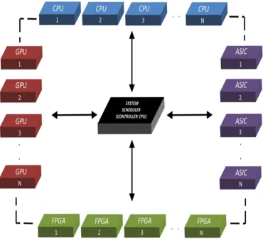
Terrestrial Intelligence). Such systems are known as heterogeneous systems. A hardware
system level diagram of a heterogeneous system with multiple CPUs, GPUs, FPGAs and
[image:13.612.134.504.195.532.2]ASICs is shown in Figure 1.
Figure 1. Hardware system level diagram of the heterogeneous system.
In section 1.1 we discuss the motivation behind using such heterogeneous systems
for high performance computing applications and pose the problem statement that we will
i.e. an optimized scheduling policy for heterogeneous systems with large degree of
heterogeneity.
1.1.
Motivation and Problem Statement
The limitations and design challenges associated with homogeneous systems; and
comparative analysis of various applications on different kinds of processors have led to
the emergence of heterogeneous systems. It has been understood that to achieve high
performance and power efficiency, different kinds of applications have different hardware
requirements. Binotto et al.[4] used a heterogeneous system of CPU, GPU and FPGA for
X-ray image processing using high-speed scientific cameras. Also, Skalicky et al. [5]
performed a distributed execution of transmural electrophysiological imaging with a
heterogeneous system comprised of CPU, GPU and FPGA. It is shown in [4], [5] and many
other works that using a heterogeneous system can give better performances in terms of
total execution time, power efficiency and system utilization as compared to homogeneous
systems.
There are many challenges of using heterogeneous systems which were presented
by Khokhar et al. [6], such as, programming, hardware platform selection, best use of large
degree of heterogeneity and network connections. Since then, many efforts have been made
at simplifying programming for platforms like CPUs, GPUs and FPGAs. These include
many libraries for CPUs, a variety of programming languages for GPUs and FPGAs in
addition to cross-compilers and high-level synthesis tools. Connecting CPU, GPU and
FPGA via PCI Express has been proposed by Chen et al. [7] and Skalicky et al. [8] to solve
graph (DAG) to heterogeneous processors have been studied and found to be NP-complete
for finding the optimal schedule [9]. Also, scheduling in heterogeneous systems has been
heavily researched [11-14], but usually only with systems containing abstract hardware
platforms. And in these studies, hardware platforms have been associated with generic
heterogeneities rather than using specific hardware platforms. As the variety of real
platforms included in current heterogeneous systems expands, the problem at hand is of
finding the best scheduling heuristic for systems with high degrees of heterogeneity.
Optimal assignment of work to hardware platforms is essential in achieving high
performance and efficiency from heterogeneous systems.
1.2.
Proposed Solution
In this work, after thorough analysis of the six state of the art scheduling policies
for heterogeneous systems and comparing their performance for a variety of stream of
applications, we propose an optimized scheduling heuristic for heterogeneous systems with
high degree of heterogeneity. The six examined policies are, predict earliest finish time
(PEFT) [15], heterogeneous earliest finish time (HEFT) [16], shortest process next (SPN),
serial scheduling (SS) [17], adaptive greedy (AG) [18] and minimum execution time/best
only (MET) [19]. In the proposed optimized heuristic, we consider a tolerance threshold,
which is the deciding metric for an assignment of task to any processor. As opposed to the
policies like SS, SPN and MET, this heuristic makes the decision to wait or to assign to
next best available processor based on a metric which ensures that the total execution time
is minimized and the system utilization is optimal. Also, this policy being dynamic, it does
capitalizes mainly on reducing communication time in the system, this policy tries to
optimize the total execution time by capitalizing on the fact that there is abundance of
multiple types of idle competing processors. This policy therefore strikes a good balance
Chapter 2
Related Work and Background
In this chapter we describe the previous work that forms the foundation of our work
and other similar efforts that are related to our objectives and contributions. In section 2.1
we discuss the related work and in section 2.2 we elaborate on the advancements in
heterogeneous computing. Section 2.3 represents the types of processors used in the
heterogeneous systems with very large heterogeneity and the methodology of classifying
dwarfs is presented in the section 2.4. Finally, in section 2.5 we present the scheduling
problem and provide a survey of the state of the art scheduling policies for heterogeneous
systems.
2.1.
Related Work
Performance evaluations have compared and contrasted various computations and
hardware platforms to determine which is best [20-22]. Skalicky et al. [23] evaluated five
linear algebra computations using multiple implementations for each hardware platform.
They presented the areas within the design space in which each processor architecture and
implementation excelled. Their results represent the ground truth for making intelligent
computation-to-hardware assignments to maximize performance. Also, Krommydas et
al.[24] evaluated the performance of four different kinds of applications on different kinds
of processors. The applications evaluated in [24] are Needleman Wunsch, GEM (Gaussian
Electrostatic Model), BFS (Breadth First Search) and SRAD (Speckle Reducing
Anisotropic Diffusion). We will use results from [23] and [24] to evaluate how well each
As opposed to the previous work [11-14], we use specific hardware platforms in
this work. Topcuoglu et al. [16] presented the highly regarded heterogeneous earliest finish
time (HEFT) policy but do not mention the heterogeneity of their system. Arabnejad et al.
[15] presented the predict earliest finish time (PEFT) policy that used a novel optimistic
cost table and produced makespans of 20% less than HEFT using an abstract system where
each platform had a heterogeneity value between 0 (similar) and 2 (very different). Liu et
al. [17] presented the priority rule based serial scheduling (SS) policy and evaluated it in a
system with uniformly distributed random task compute times. Wu et al. [18] presented the
adaptive greedy (AG) algorithm and evaluated it in a heterogeneous system of CPU+GPU
workstations but used exponentially distributed random task compute times. Braun et al.
[19] presented eleven scheduling policies including opportunistic load balancing (OLB)
and minimum execution time (MET) and evaluated them in a system with uniformly
distributed random task compute times. However, OLB does not consider the execution
time of each task on the given hardware platform before making assignments. The shortest
process next (SPN) policy was suggested by Khokhar et al. [6] for use in heterogeneous
systems and improves upon OLB by choosing the next task to assign based upon the
shortest execution time of a task on any of the available hardware platforms.
2.2.
Heterogeneous Computing
Until very recently, the most powerful HPC (High Performance Computing)
systems were primarily CPU based [25], although there is a very recent but significant shift
towards the use of general-purpose graphical processor unit (GPU) co-processing. On the
the true compute power of a cluster [26]. Because power consumption, and hence heat
generation, is proportional to clock speed, processors have begun to hit the so-called “speed
wall”. Meanwhile, hardware accelerators have occupied niches, such as video processing
and high-speed DSP applications. The most commonly available of these accelerators are
the (general-purpose) graphical processor unit (GPU) and the FPGA.
Systems that use more than one kind of processor are referred to as heterogeneous
computing. These are multi-core systems that gain performance not by just adding more
cores, but also by including specialized processing capabilities to handle specific tasks.
There are a number of platforms that implement an on-chip or off-chip heterogeneous
CPU+GPU+FPGA system. A sophisticated sixteen node cluster, known as the
“Quadro-Plex Cluster” [27] is an example of such a heterogeneous system. It has two 2.4 GHz AMD
Opteron CPUs, four nVidia Quadro FX5600 GPUs, and one Nallatech H101-PCIX FPGA
in each node, with a thread management design matching that of the GPUs. Another such
example is the “Axel” [28]. It is a configuration of sixteen nodes in a Non-uniform Node
Uniform System (NNUS) cluster, each node comprising an AMD Phenom Quad-core
CPU, an nVidia Tesla C1060, and a Xilinx Virtex-5 LX330 FPGA. Also, the “chimera”
[29] is another example of a heterogeneous system of CPU, GPU and FPGA.
2.3.
Types of Processors
Different kinds of processors have their own purpose in any system and therefore
their own set of advantages and disadvantages. The general-purpose CPU is expected to
perform a variety of tasks and therefore CPU processor designs cannot afford to specialize.
for general almost all kinds of computational loads. CPUs are usually deeply pipelined, run
at very high clock frequencies and have a lot of hardware on-board, etc. to run code
speculatively/out of order. CPUs are very useful and perform the best when there is a lot
control switching in the application, pointer usages, indirect load-stores etc.
Traditionally developed for graphics processing, GPUs today are used for almost
any application which has lots of parallelism. This is because GPUs were designed to have
a SIMD (Single Instruction Multiple Data) architecture with the vision to efficiently
perform linear operations on vectors and matrices. Also, they use a lot less power when
compared to CPUs for similar computations [30]. GPUs have hundreds or even thousands
of stream processors, and each stream processor runs slow when compared to a CPU and
also has less features; but collectively, the extremely high degree of parallelism in GPUs
hide the latency and outperform CPUs in tasks with lots of parallelism.
An FPGA is very different from CPUs or GPUs in the sense that it is not a processor
in itself i.e. it does not run a program stored in the program memory. FPGAs are special
hardware implementations of specific algorithms/tasks and are more deterministic. Being
special hardware implementations, they are faster than any software implementation. Also,
they can be configured as needed and this makes them ideal for re-configurable computing
and application specific processing. Another benefit of the custom design is that high
performance can be achieved at lower frequency.
2.4.
Dwarfs
The applications chosen for our work belong to multiple domains, ranging from
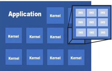
know that each application can be broken down to a set of kernels and that each kernel in
an application has a particular computational objective for which it follows a computation
and communication pattern. This idea of breaking down an application into kernels where
[image:21.612.96.527.211.483.2]each kernel has a computational objective is illustrated in Figure 2.
Figure 2. Application break down: an application has multiple kernels; each kernel
has multiple instructions (INS).
An algorithmic method that captures a pattern of computation and communication
is called a dwarf. In his work [31], P. Colella identified seven numerical methods that he
seven dwarfs can be understood as equivalence classes in which membership in a class is
defined by the similarity in the computation and communication pattern i.e. data
movement. Inspired from [31] and after exploring more applications, Asanovic et al. [32]
expanded the list of dwarfs from seven to thirteen. Kernels that are members of a class can
have different implementations and the core numerical methods may change too, but the
underlying patterns have persisted for generations and will remain important in the future
too. Below, with short descriptions, we list all the dwarfs presented in [32] and the dwarfs
marked with * are the dwarfs that were newly introduced.
a) Dense Linear Algebra: These are traditional vector and matrix operations,
usually divided into three levels. The three levels are level 1 (vector/vector),
level 2 (matrix/vector) and level 3 (matrix/matrix) operations.
b) Sparse Linear Algebra – Sparse matrices are the ones that have many zero
entries. Sometimes, using another data structure has more advantages when it
comes to memory and efficiency. Algorithms that involve such data structures
and computations belong to sparse linear algebra category of dwarves.
c) Spectral Methods – These methods are widely used in many different fields
like applied mathematics and scientific computing. In this method, data is
operated on in the spectral domain, which is often transformed from a temporal
or a spatial domain. Therefore, they often involve use of a Fast Fourier
Transform (FFT).
d) N-Body Methods – These methods involve calculations that depend on
interactions among many discrete points. This dwarf does not cover a few
e) Structured Grids – In this dwarf, data is formatted in a regular
multidimensional grid. This grid is updated in a sequence of steps and in each
step, the points are updated using values from its neighborhood.
f) Unstructured Grids – These methods are used when there are surfaces/objects
or any modelling problem that has irregular geometric dimensions. When each
grid element is updated, unlike structured grids, irregular number of
neighboring elements are accessed, leading to an irregular amount of
computations.
g) MapReduce – Initially, this dwarf was known as “Monte Carlo” after the idea
of using statistical methods based on repeated random trials. Generalizing the
same idea, this dwarf has the programming model in which a function is
repeatedly executed independently and the results are aggregated at the end
from all these independent executions.
h) Combinational Logic * - This dwarf has many important functions that exploit
bit-level parallelism for high throughput. These dwarfs have computations in
which the operations are quite simple logical operations, but they are operated
on very large amounts of data.
i) Graph Traversal * - These are kernels which traverse a number of objects in a
graph data structure while examining the characteristics of the objects, usually
with very little computation.
j) Dynamic Programming * - Dynamic programming is a programming method
problems. Subsequently, combining the solutions to the sub problems provides
the solution to the original problem.
k) Backtrack and Branch-and-Bound * - These algorithms are very effective in
solving search and optimization problems. The idea is to search for an objective
in a very large space to find an optimal solution. Usually the search space is
intractably large and a set of rules are devised to prune subregions of this search
space that have no helpful solutions. This method uses the divide and conquer
rule to divide the search space into smaller regions and then searches for
solution in this smaller sub region.
l) Graphical Models * - These models are represented by a graph that has nodes
which represent variables and edges that represent conditional probabilities. As
these models are graphs, they are evaluated using graph traversal methods.
m) Finite State Machines * - This is a system that can be described as set of
connected states. The behavior of such systems can be defined by states,
transitions defined by inputs and the current state, and various events associated
with transitions or states.
Understanding these dwarfs and the idea that applications consist of one or more
kernels is key in identifying the dwarfs that are found in an application. This means, that
an application can have kernels that belong to different kinds of dwarfs. For example,
consider a Bayesian network model for a machine learning problem. This application has
both, the graphical model dwarf which builds the model during the training of the system
and the graph traversal dwarf that evaluates during the testing phase of the system. But
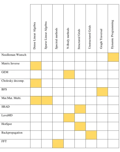
Table 1. Each column denotes the types of dwarfs and each row shows the
belongingness of applications to dwarfs.
be the BFS implementation for the shortest path problem which has just the Graph
Traversal dwarf. Going forward with this idea, the Table 1. summarizes a variety of
examples of applications. It also indicates all the dwarfs that are found in all these
applications.
2.5.
Scheduling
2.5.1 Problem Representation
We can represent the problem of scheduling kernels from an application in a
heterogeneous system as (R | prec | Cmax) in standard scheduling notation. For this problem,
we have processors pj ∈ P for 1 ≤ j ≤ np, where np is the number of processors in the
system, and a dataflow graph G = (V, E) where V is the set of kernels and E is the set of
dependencies between kernels. Each kernel vi ∈ V has an execution time tij ∈ T for
processor j. For kernel vi, the data transfer cost is djk∈ D when vi’s predecessor is assigned
to processor pjand viis assigned to pk.
Mathematically a scheduling algorithm can be represented as a function f that maps
kernels from V to processors in P as f : V → P such that each kernel is assigned to exactly
one processor. Currently there are no feasible polynomial time algorithms to find the best
kernel-to-processor assignment map, or schedule, by minimizing the maximum completion
time of any kernel in the application. We do not find a lot of previous work focused on this
problem in particular since the two relaxed simplifications still have no known polynomial
time solutions. In essence, this work presents an approach that models the performance of
statically, having access to the entire kernel dataflow graph (DFG) of the application. In
the real world though, this may not be possible, so dynamic scheduling approaches are also
used in large number of systems.
Foster [33], Puigjaner [34] and many others have been active researchers in
modeling system performances. Ideally, the scheduling should be able to assign the kernels
to the processor to achieve the lowest overall execution for the stream of applications. Since
we cannot achieve the minimum execution time in real world, efforts have been made to
identify the components of this overall execution time. We have understood that this
overall execution time comprises of three parts: kernel compute time, data transfer time,
and scheduling delay. The first two components, kernel compute time and data transfer
time depend on the processors in the system and the system design. Therefore, we will only
discuss the scheduling delay; the first two components being trivial. This delay, 𝜆, as
discussed earlier could be caused by various factors such as:
• the scheduling delay to process which task should be assigned to which processor
next,
• communication delay from the scheduler to the processor to tell it to begin
processing and provide the necessary information,
• dependencies on kernels that are being executed in another processor, but have not
completed yet.
This means that the order in which tasks are assigned impacts the amount of
scheduling delay. To understand this delay and its impact on the performance of scheduling
policies, we compare the overall impact of this delay on the total execution time for each
2.5.2 Types of Scheduling Policies
Elaborating a little more on types of scheduling policies, static scheduling policies
have access to the entire DFG of the application prior to execution. This category therefore
determines a schedule before executing the application on the heterogeneous system. The
schedule that the policy gives beforehand, is followed during the actual execution. Some
notable work in this category of scheduling policies was by Herrmann et al. [35] and Liu
et al.[17]. Herrmann et al. investigated scheduling with a peculiar chain dependency
structure and Liu et al. proposed a priority rule-based algorithm which had arbitrary
dependencies. As compared to the policies mentioned before, dynamic scheduling policies
do not have access to the entire DFG. These policies therefore try to make the best of the
current state of the system and the kernels that have been already submitted. Adaptive
Greedy and Adaptive Random were two policies presented in [18] by Wu et al. The
Adaptive Greedy policy tries to minimize the waiting time for each kernel whereas the
Adaptive Random policy uses random weights and probabilities to assign kernels. The
system used for this investigation had multiple CPUs and GPUs. But in an approach like
this, the kernels become resource constrained and need a different scheduling approach
[36]. This is mainly because the kernels are custom and cannot be broken further down in
a combination of standard library routines.
2.5.3 Chosen Scheduling Policies
In this work we analyze two static and four dynamic state of the art scheduling
policies to assign kernels to processors. All of these policies assign kernels from a set of
subset of V. It is a set in which each kernel that has not yet begun execution and whose
dependencies, also known as the precedence constraints, have already been completed. The
set of available processors, A, is a subset of P. It contains only those processors that have
are not currently executing any kernels or data transfers.
The shortest process next (SPN) policy was suggested by Khokhar et al. [37]
chooses a kernel from I that has the minimum execution time on any of the processor from
A. If there is any processor available and there are kernels in set I, assignments are made
to keep the system busy. This policy tries to minimize 𝜆delays by keeping the processor
busy. But this policy has its own decision making mechanism, according to which it does
not use the information about the difference in execution time among the processors. This
mechanism therefore disregards the observed heterogeneity observed in the kernels,
therefore not making the best use of available heterogeneity in the system architecture.
Braun et al. [19] presented the minimum execution time (MET) policy. In this
policy, a kernel is chosen in a random order from I and is then assigned to the processor
with the lowest execution time for that kernel. As opposed to SPN, if the best suited
processor for the kernel is not currently available, policy decides to wait for the best
processor to become available i.e. the kernel will be assigned to that best processor at a
later time. By virtue of this rule, a processor sits idle if there are no kernels in I that are
suitable for it. This policy always waits to assign kernels to their best processor. Due to the
large differences in execution times, this will result in lower 𝜆delays.
A relatively more statistical scheduling policy known as serial scheduling (SS) was
presented by Liu et al. [17]. In this policy, the metric for decision making is the standard
standard deviation of the compute times are calculated for each
kernel-to-available-processor mapping. Then the scheduler chooses the kernel from I with the highest standard
deviation and assigns it to the processor from A in which the kernel has the lowest execution
time. Whenever there are kernels in I and there are available processors, assignments can
be made in this policy. This policy is a little different than the policies mentioned
previously. It does not directly consider the difference in execution time among the
processors in its calculations; instead calculates the standard deviation in execution time
among the processors and assigning kernels to the processor with the least execution time.
When the best processor is busy, just like SPN, SS assigns kernels to processors even if
they are the not the best choice.
The adaptive greedy (AG) policy presented by Wu et al. [18] tries to optimize the
data transfer and queuing delay. It maintains queues for each processor and attempts to
make assignments to minimize data transfer and queuing delay. The policy calculates wait
time by adding the queuing delay for each processor and the associated data transfer time
for the given data size and transfer rate. Then the policy chooses the processor which will
incur the lowest total time. The queuing delay mentioned above is calculated as the sum of
the compute times for all kernels already in the queue for each of the processors. This
policy takes the differences in execution time between the various processors into account
by using the queuing delay in its decision making metric. As it turns out, this policy
indirectly ends up making the decision to wait for the best processor.
In [18], AG considers a CPU-GPU system, but we generalize the policy to a
heterogeneous system with CPU, GPU and FPGA. This policy examines every device in
the device g. As shown in (1),𝜏𝑔 comprises of the queueing delay 𝜏𝑔𝑞 (time to queue the
kernel to the processor g) and the data transfer delay 𝜏𝑔𝑑 (time to transfer the data that the
kernel requires for successful execution). Also (2) explains that 𝜏𝑔𝑞, the queueing delay is
estimated by the number of kernel calls queued on that processor i.e. Ngand the average
execution time of the last k kernel calls on that processor i.e. 𝜏𝑔𝑘.
𝜏𝑔 = 𝜏𝑔𝑞+ 𝜏𝑔𝑑 (1)
𝜏𝑔𝑞 = 𝑁𝑔. 𝜏𝑔𝑘 (2)
The heterogeneous earliest finish time (HEFT) policy presented by Topcuoglu et
al. [16] is a static scheduling policy which makes its decisions based on a statistically
derived rank. Because the policy is static, it has access to the entire kernel DFG beforehand,
and using this DFG, the policy first statically ranks all kernels and then assigns them to
processors in order of highest rank first in I. The assignments are made to the processor
from A with the least sum of time remaining of any previous kernel and execution time of
the current kernel on that processor. This policy was specifically designed to minimize the
𝜆 delays in the rank calculations by evaluating dependencies in the DFG.
Tasks in HEFT are ordered based on their scheduling priorities using their upward
and downward rank. The upward rank of a task 𝑛𝑖is defined by (3), where succ(ni) is the
𝑟𝑎𝑛𝑘𝑢 (𝑛𝑖) = 𝑤𝑖+ max 𝑛𝑗 𝜖 𝑠𝑢𝑐𝑐(𝑛𝑖)
(𝑐𝑖,𝑗+ 𝑟𝑎𝑛𝑘𝑢 (𝑛𝑗)) (3)
set of immediate successors of 𝑛𝑖, 𝑐𝑖,𝑗 is the average communication cost of edge (i, j), and
𝑤𝑖 is the average computation cost of 𝑛𝑖. It is called the upward rank because it is computed
recursively traversing the graph upward, starting from the exit task. The upward rank for
𝑟𝑎𝑛𝑘𝑢 (𝑛𝑒𝑥𝑖𝑡) = 𝑤𝑒𝑥𝑖𝑡 (4)
Similarly, the downward rank is defined by
𝑟𝑎𝑛𝑘𝑑(𝑛𝑖) = max
𝑛𝑗 𝜖 𝑝𝑟𝑒𝑑(𝑛𝑖)
(𝑟𝑎𝑛𝑘𝑑 (𝑛𝑗) + 𝑤𝑗+ 𝑐𝑗,𝑖) (5)
where pred(ni) is the set of immediate predecessors of task ni. It is called the downward
rank because it is computed recursively traversing the graph downward, starting from the
entry task of the graph. The downward rank value for the entry task nentry is zero. From
these definitions, we understand that the upward rank is the length of the critical path from
ni to the nexit, including the computation cost of the task ni. And the downward rank is the
longest distance from nentry to ni, excluding the computation cost of the task itself. After
selecting the task based on its calculated priority (using the upward and downward rank),
the processor selection phase of HEFT is a little different than most other scheduling
policies. It has an insertion-based policy which considers an insertion of task in an earliest
time slot between two already scheduled tasks, if the time slot can accommodate the
computation time of the chosen task.
The predict earliest finish time (PEFT) policy, yet another static policy, presented
by Arabnejad et al. [15] follows a similar process to HEFT except that the ranks are based
on a pre-computed cost table. This cost table serves as a lookup table that helps the policy
in making decisions for allocation of kernel to the processor. The assignments are made to
the processor from A with the least sum of value from the cost table and execution time of
the kernel on that processor. Just like HEFT, this policy also specifically addresses 𝜆delays
PEFT uses an optimistic cost table (OCT) based on which the task priority is
decided and the processor is selected. The OCT is a matrix in which the rows indicate the
number of tasks and the columns indicate the number of processors. Each element in the
matrix OCT(ti, pk) is the maximum of the shortest paths to ti children’s tasks to the exit
node in the case that the task ti is assigned to processor pk. This value is defined by the
formula shown in (6) by traversing the task graph from the exit task node to the entry task
node. In (6), 𝑐𝑖,𝑗 is the average communication cost, 𝑤(𝑡𝑗, 𝑝𝑤) is the execution time of task
tj on processor pw, succ(ti) is the set of immediate successors of ti and P is the number of
processors in the system. Also 𝑐𝑖,𝑗 is zero if tj is being evaluated for processor pk because
𝑂𝐶𝑇(𝑡𝑖, 𝑝𝑘) = max 𝑡𝑗𝜖 𝑠𝑢𝑐𝑐(𝑡𝑖)
[min
𝑝𝑤𝜖𝑃
{𝑂𝐶𝑇(𝑡𝑗, 𝑝𝑤) + 𝑤(𝑡𝑗, 𝑝𝑤) + 𝑐𝑖,𝑗}] ,
𝑐𝑖,𝑗 = 0 𝑖𝑓 𝑝𝑤 = 𝑝𝑘 (6)
the task is going to be executed on the same processor and therefore there is no
communication cost. And finally to make assignments, task priority is calculated using
rankoct which is defined in (7). To select a processor for a task, OEFT (Optimistic Earliest
𝑟𝑎𝑛𝑘𝑜𝑐𝑡(𝑡𝑖) =
∑𝑃𝑘=1𝑂𝐶𝑇(𝑡𝑖, 𝑝𝑘)
𝑃 (7)
Finish Time) is calculated which sums to EFT the computation time of the longest path to
the exit node. Comparing ranku and rankoct, it is understood that ranku uses the average
computing cost for each task and also accumulates the maximum descendent costs of
descendent tasks to the exit node. In contrast, rankoct is an average over a set of values that
were computed with the cost of each task on each processor.
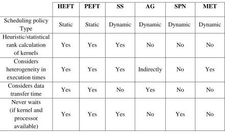
A comparative analysis of the before mentioned policies can be found in Table 2.
to processors. Each column in the table represents a scheduling policy. This comparison
helps in understanding the key differences in all these policies and the effects of these
differences in the performance of these policies.
[image:34.612.86.527.233.497.2]
Table 2. Summary of key properties of the scheduling policies HEFT, PEFT, SS,
AG, SPN and MET.
HEFT PEFT SS AG SPN MET
Scheduling policy
Type Static Static Dynamic Dynamic Dynamic Dynamic Heuristic/statistical
rank calculation of kernels
Yes Yes Yes No No No
Considers heterogeneity in execution times
Yes Yes Yes Indirectly No Yes
Considers data
transfer time Yes Yes No Yes No No
Never waits (if kernel and
processor available)
Yes Yes Yes No Yes No
From the before mentioned descriptions and Table 2, we understand that static
policies i.e. HEFT, PEFT; have a ranking mechanism like a preprocessing step to prioritize
the available set of subtasks in the application. Using the ranks from the ranking process,
a fixed static schedule is formed and is followed during the execution. But for applications
with high degree of parallelism and very deep DFG, the ranking step can be very time
consuming and thus cumulatively very expensive. Among the dynamic policies, Serial
this ranking is not iterative and neither is it as complicated as it is for the static policies.
This policy tries to prioritize execution of kernels that have the maximum heterogeneity on
a processor that is available and has the least execution time than the other available
processors. While doing this, the policy might end up assigning kernels to a processor that
is very expensive in terms of computation time. Shortest Process Next (SPN) has a simple
rule for assignment i.e. assign the shortest available kernel to the best available processor.
In this process, the policy does not consider the heterogeneity available in the system and
therefore does not make the most effective use of the resources available. In both the
policies, SS and SPN, the assignments are made at the cost of not caring about how slow
the selected processor is as compared to most suitable processor which is currently
unavailable. As opposed to SS and SPN, Minimum Execution Time (MET) has an even
simpler approach of choosing the best processor for a kernel, whenever it is available, even
at the cost of waiting time. This approach makes the best use of heterogeneity of the system,
but will have large execution times when few processors are best at many different kernels,
adding a lot of waiting time. When all other policies concentrate on reducing the execution
time or execution time coupled with communication time, Adaptive Greedy (AG) tries to
reduce waiting time for kernel execution and not computation time across processors.
Therefore, the policy favors executing kernels on either the same processor or the
processors connected with higher bandwidths. All the above mentioned dynamic policies
have access to the observed heterogeneity in the kernels and multiple types of processors.
But none of these policies capitalize on this heterogeneity among kernels and the
Chapter 3
Alternative Processor within Threshold (APT)
In this chapter, section 3.1 describes the proposed scheduling heuristic, Alternative
Processor within Threshold (APT) and in section 3.2 discusses the methodology to use the
heterogeneous system and evaluate the seven scheduling policies (six state of the art
examined policies and the proposed policy - APT).
3.1.
Scheduling heuristic - Alternative Processor within Threshold
(APT)
In this section, we introduce a new scheduling heuristic for heterogeneous systems,
called Alternative Processor within Threshold. APT is a dynamic scheduling heuristic that
adds flexibility to MET, a flexibility that can be tuned to the degree of heterogeneity of the
system. This flexibility offered by APT, makes it more lenient in making the
kernel-to-processor assignment instead of always waiting for the best suitable kernel-to-processor to be
available. This policy has just one phase, the processor selection phase, to choose a
processor which will execute the selected task.
Ideally, for a scheduling policy to be effective and reduce the overhead of
scheduling delay, the scheduling policy should be quick in choosing the task and the
processor on which the task will be executed. This means that, if the policy has lesser
computations in selecting the task to be scheduled and a suitable processor, it reduces the
λ delay, thus achieving better performance. But this improvement can come with the cost
assignment is not good enough. To address this issue, we try to keep the computations in
the processor selection phase to a minimum in our policy.
APT maintains a list of tasks as and when they arrive for execution. This list can be
referred to as a queue because it is filled on first-come, first-serve basis while maintaining
the computational and data dependencies among different kernels. If there are tasks that
are ready to be scheduled, each task in this queue gets a fair chance to find a suitable
processor for execution. Once there are tasks that can be scheduled, the policy tries to find
a suitable processor for the task in the processor selection phase.
For a chosen task vi from the queue, the processor selection phase, tries to find a
processor which has the minimum execution time for vi. The minimum execution time can
be found from the entries for vi in the lookup table and we refer to the processor with the
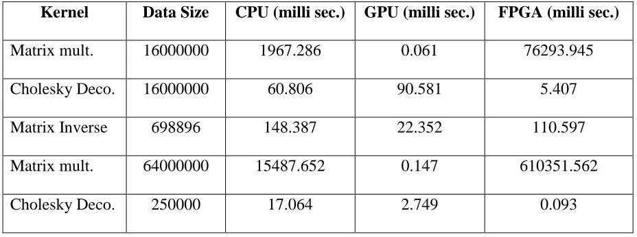
minimum execution time as pmin. The lookup table is a table that consists of the execution
times for different kernels (for different data sizes) on different processors. Table 3. shown
[image:37.612.79.543.485.658.2]below is an example of such a lookup table.
Table 3. Lookup table example.
Kernel Data Size CPU (milli sec.) GPU (milli sec.) FPGA (milli sec.)
Matrix mult. 16000000 1967.286 0.061 76293.945
Cholesky Deco. 16000000 60.806 90.581 5.407
Matrix Inverse 698896 148.387 22.352 110.597
Matrix mult. 64000000 15487.652 0.147 610351.562
The complete lookup table is shown in Appendix A. In this table, each row indicates
the execution times of a kernel for a data size on different processors, in this case, the
processors are CPU, GPU and FPGA. For example, the third row indicates the execution
times in milliseconds for the matrix inversion kernel for a matrix that has 836 rows and
836 columns, therefore the data size is 836*836 i.e. 698896.
In an ideal case, if pmin is available (it is not executing any other kernel) then vi is
assigned to pmin. But pmin can be busy executing some other task vk and now the policy has
to make the critical decision to wait for this processor to be available or to assign the task
to alternative processor (second best processor). APT uses threshold i.e. a threshold
constant (customizable as per policies demand), that decides if vi should be allocated to
alternative processor (palt) or should the policy wait for pmin to be available for execution.
Trying to allocate the task to an alternative processor is the difference in APT when
compared to MET and this alternative processor can keep the system busy, while also
reducing the waiting time.
The concept of finding the alternative processor is very important in understanding
APT’s functioning. If 𝒙 is the execution time of kernel vi on pmin (which can be found from
the lookup table), then the threshold for kernel vi, can be defined by (8)
𝑡ℎ𝑟𝑒𝑠ℎ𝑜𝑙𝑑 = 𝛼 ∗ 𝑥 ,
𝑤ℎ𝑒𝑟𝑒 𝛼 ≥ 1 (8)
where α is the customizable variable that can take any value greater than or equal to 1.
Also, if vi is dependent on some previous task (vprev executing on processor pprev) for data,
then the transfer time for that data from pprev to the contending processors is also very
processor for which the addition of execution and the data transfer times is less than or
equal to the policy’s established threshold, and is available to execute kernel vi”. The
purpose of defining a threshold is to address the trade-off between waiting for the best
processor and assigning the task at hand to an alternative processor. α’s value determines
how large or small the threshold is, which governs the degree of flexibility of the heuristic
in choosing the alternative processor. As we will see, this degree of flexibility will affect
the efficiency of the scheduling policy depending highly on the degree of heterogeneity of
the system. The proposed algorithm for APT is formalized in Algorithm 1.
Algorithm 1. The APT Algorithm
1: const threshold = αx 2: while(true)do
3: collect DFGs of all incoming jobs 4: for (all available kernels in DFG) do 5: pmin ← findBestProc(kernel)
6: if there is a pmindo
7: allocate current kernel to pmin
8: remove current kernel from available list
9: else do
10: palt ← find2ndBestProc(kernel, threshold)
11: if there is a palt do
12: allocate current kernel to palt
13: remove current kernel from available list
14: end if
15: end if
The algorithm starts by setting the threshold for the policy and then it is always
waiting for new tasks to be allocated to the processors. In line 4 we see that the policy
iterates through all available kernels that are waiting for execution. The policy tries to find
pmin for the kernel using the function findBestProc in line 5 and allocates the kernel to pmin
if pmin is available in lines 6 and 7. Later in line 8, the kernel is removed from the list of
available kernels. If pmin was not available, we see that the policy tries to find the alternative
processor (palt) with the function find2ndBestProc in line 10. If it finds palt, the policy
allocates the kernel to palt in line 12. And in line 13, the kernel is removed from the list of
available kernels.
A closer look at the algorithm can help us understand that a larger threshold means
that in the case when pmin is not available, the policy is willing to sacrifice on the least
execution time rather than waiting. And a smaller threshold signifies that the policy is very
stringent in choosing the alternative processor and is not designed to allow a lot of slack in
terms of execution time of the kernel. But the overall effect of the threshold is influenced
also by the heterogeneity of the system. To get the best results, a good balance of α value
is to be found with respect to the heterogeneity of the system. This effect is explained in
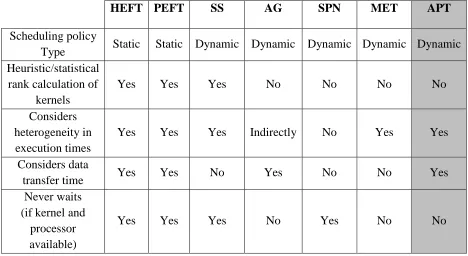
detail in chapter 4 with the experimental results. In Table 4 shown below, we see the
Table 4. Summary of key properties of the scheduling policies HEFT, PEFT, SS,
AG, SPN, MET and APT
HEFT PEFT SS AG SPN MET APT
Scheduling policy
Type Static Static Dynamic Dynamic Dynamic Dynamic Dynamic Heuristic/statistical
rank calculation of kernels
Yes Yes Yes No No No No
Considers heterogeneity in
execution times
Yes Yes Yes Indirectly No Yes Yes
Considers data
transfer time Yes Yes No Yes No No Yes
Never waits (if kernel and
processor available)
Yes Yes Yes No Yes No No
3.2.
Methodology
In this section we establish the method of evaluating the performance of scheduling
policies for a heterogeneous system. With the help of the work by Skalicky et al.[5], we
have developed a software to simulate the distributed hardware heterogeneous system, the
incoming stream of applications as a work load for the system and the different scheduling
policies.
The simulated heterogeneous system comprises of commercial-off-the-shelf
(COTS) CPUs, GPUs and FPGAs and each communication link is based on PCI Express
(PCIe). The number of processors of any type are customizable in the software and so is
for any kind of heterogeneous system with different kinds of processors. For our work, we
have used the system with one CPU, one GPU and one FPGA.
A stream of applications serves as an input to the scheduler of the heterogeneous
system. This stream of applications can be represented as a DFG (Data Flow Graph) of
kernels. An input stream can have multiple applications and each application can have
multiple similar or distinct kernels. The kernels within the application can be independent
of one another too and applications may have data or computational dependencies among
them. This input stream can have as many applications, and there is no specific number of
instances or order in which the applications occur. We have used two types of input streams
for our work, 1. input stream without any dependencies and 2. input streams with
dependencies, which we will henceforth refer to as DFG Type-1 and DFG Type-2
respectively. To generate each type of input stream, we have written a software which
accepts for an input, a series of kernels and each kernel has its own data size. This series
of kernels is then fit into the model/type of DFG, either DFG Type-1 or DFG Type-2, as
needed. The series of kernels given as input, has different number of kernels and different
data sizes for each kernel.
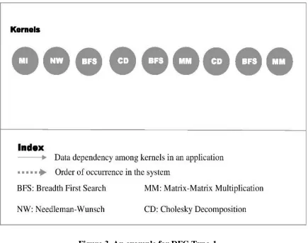
If there are a total of n kernels in the input, then the graph generated of DFG
Type-1 will have n-1 kernels available for execution in parallel with no data or computational
dependencies (referred to as level-1) and only after these kernels are executed, the last nth
kernel is available for execution. An example of DFG Type-1 with 9 kernels can be seen
Figure 3. An example for DFG Type-1.
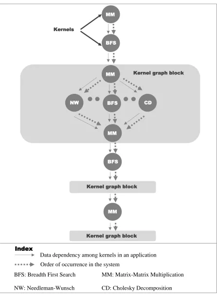
there are n kernels in the input, then the graph generated of DFG Type-2 will have data and
computational dependencies among kernels as shown in figure C. There are individual
kernels and a group of kernels with computational and data dependencies. There is also a
kernel graph block with a diamond like structure with one kernel each at the top and
bottom, and multiple independent kernels in the middle. There are three such kernel graph
blocks in any graph in Figure 3, where 9 kernels are available for execution in parallel and
Figure 4. An example for DFG Type-2.
Kernels
MM
BFS
MM
NW CD
Index
Data dependency among kernels in an application
Order of occurrence in the system
BFS: Breadth First Search MM: Matrix-Matrix Multiplication
NW: Needleman-Wunsch CD: Cholesky Decomposition
BFS
MM
BFS
Kernel graph block
Kernel graph block
MM
a total of n kernels in the input, then the graph generated of DFG Type-2 will have data
and computational dependencies among kernels as shown in figure C. There are individual
kernels and a group of kernels with computational and data dependencies. There is also a
kernel graph block with a diamond like structure with one kernel each at the top and
bottom, and multiple independent kernels in the middle. There are three such kernel graph
blocks in any graph of DFG Type-2, just as shown in figure 4. When the number of kernels
in the input changes, the structure remains the same, for both the types of graphs. The only
thing that changes is the number of kernels in level-1 in DFG Type-1 and the independent
kernels in kernel graph blocks of DFG Type-2.
The graphs generated using the above-mentioned software serve as the input to the
scheduling policy. These graphs have different kernels in different orders and each kernel
[image:45.612.73.552.429.658.2]has different data size, therefore ensuring that the scheduling policies are evaluated without
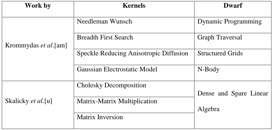
Table 5. Kernels chosen in our work
Work by Kernels Dwarf
Krommydas et al.[am]
Needleman Wunsch Dynamic Programming
Breadth First Search Graph Traversal
Speckle Reducing Anisotropic Diffusion Structured Grids
Gaussian Electrostatic Model N-Body
Skalicky et al.[u]
Cholesky Decomposition
Dense and Spare Linear
Algebra Matrix-Matrix Multiplication
any bias and the results can be extrapolated to any stream of applications. We have 10
input graphs for both, DFG Type-1 and DFG Type-2; generated using the software
described above and each graph of a type has different order and number of kernels. The
kernels that are chosen to be a part of the workload for the stream of applications are shown
in Table 5.
We give a brief understanding of these kernels in the following paragraphs.
• Needleman-Wunsch (NW) - The Needleman-Wunsch algorithm is a dynamic
programming algorithm for optimal sequence alignment [38]. This algorithm is a
nonlinear global optimization method that is used for amino acid sequence
alignment in proteins. Because the Needleman-Wunsch algorithm finds the optimal
alignment of the entire sequence of both proteins, it is a global alignment technique,
and cannot be used to find local regions of high similarity.
• Breadth First Search (BFS) - Breadth First Search is an algorithm to traverse a
graph in search of a node or a path, usually starting from its root node. In this
algorithm, all immediate unvisited neighbors are inspected. Subsequently, for each
of these neighbors, their own unvisited immediate neighbors are visited, eventually
traversing the entire graph. The traversing is terminated depending on the problem
statement, for example, if the algorithm is used to find for a particular node, then
the algorithm terminates if the node is found or if the entire graph is traversed and
still the node wasn’t found.
• Speckle Reducing Anisotropic Diffusion (SRAD) - Speckle Reducing Anisotropic
Diffusion, also known as SRAD is an algorithm based on partial differential
and radar imaging applications. It is the edge-sensitive diffusion for speckled
images. This is similar in ways that the conventional anisotropic diffusion is the
edge-sensitive diffusion for images corrupted with additive noise. Apart from
perfectly preserving edges, SRAD also enhances edges by inhibiting diffusion
across edges and allowing diffusion on either side of the edge.
• Gaussian Electrostatic Model (GEM) - Electrostatic interactions are a very
important factor in determining properties of biomolecules. The ability to compute
electrostatic potential generated by a molecule is often essential in understanding
the mechanism behind its biological function such as catalytic activity or ligand
binding. Gaussian Electrostatic Model, also referred to as GEM, calculates the
electrostatic potential of a biomolecule as the sum of charges contributed by all
atoms in the biomolecule owing to their interaction with a surface vertex (two sets
of bodies)
• Cholesky Decomposition (CD) - The Cholesky decomposition [39] of a positive
definite matrix A is an upper triangle matrix U with only positive diagonal values
such that it satisfies (9).
𝐴 = 𝑈𝑇𝑈 (9)
• Matrix - Matrix Multiplication (MatMul) – The purpose of the kernel is singular
i.e. multiplying two matrices, and the operations (instructions) involved in this
kernel are very simple too. but, it is one of the most highly used kernels in a variety
of domains including image processing, machine learning, computer vision, Finite
• Matrix Inverse (MI) – Like MatMul, this again is one of the most widely used
kernels across domains. The inverse of the matrix A is denoted by A-1 such that,
𝐴 𝐴−1 = 𝐼 (10)
where I is an identity matrix of the same dimensions as that of A.
We use these kernels in the stream of applications and their execution times in the lookup
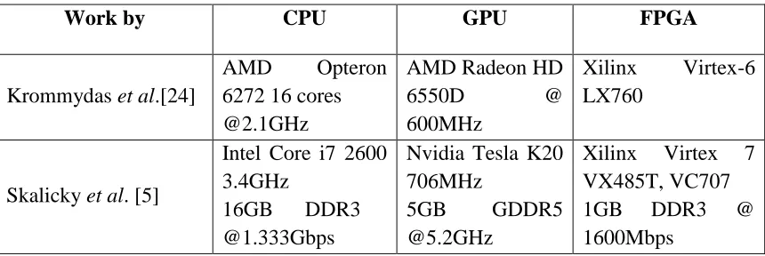
table. These execution times used for our work for the following hardware platform
[image:48.612.92.522.292.436.2]specifications:
Table 6. Hardware platform specifications.
Work by CPU GPU FPGA
Krommydas et al.[24]
AMD Opteron
6272 16 cores @2.1GHz
AMD Radeon HD
6550D @
600MHz
Xilinx Virtex-6 LX760
Skalicky et al. [5]
Intel Core i7 2600 3.4GHz
16GB DDR3 @1.333Gbps
Nvidia Tesla K20 706MHz
5GB GDDR5
@5.2GHz
Xilinx Virtex 7 VX485T, VC707
1GB DDR3 @
1600Mbps
In our work, we have made a generalization that the execution time for any given
kernel belongs to the category of the platform. What this means is that, we have the
execution times on the Intel Core i7 2600 CPU for the kernel matrix-matrix multiplication
from the work of Skalicky et al.[5], and not on AMD Opteron 6272 (CPU used by
Krommydas et al.[24]); but we will assume that this is the execution time for the category
CPU, irrespective of the exact CPU configuration. Similarly, we will also assign the
execution times to the categories GPU and FPGA, and not the specific configuration of
Using PCIe 2.0 the data rate per lane is 500MBps, we varied the number of lanes
to be 8 and 16 so that we can understand the effect of varying the data transfer rates on the
performance of APT. With 8 lanes (x8) this would achieve an approximate throughput of
4GBps (500 × 8) and with 16 lanes (x16) this would achieve an approximate throughput
of 8GBps (500 × 16). In our work, we maintain the data transfer rates between all
processors to be the same i.e. if the rate is 4GBps, then it is the same from the CPU to GPU,
GPU to FPGA and CPU to FPGA.
Once the system starts receiving computations that are to be executed, it is the job
of the scheduler to assign tasks to a processor and this decision of assignment of any task
to a particular processor is made by the scheduling policy. Each scheduling policy has its
own strategy to make assignments. This scheduler also has access to a lookup table which
has real execution times of a variety of kernels (each belonging to some dwarf category)
from the works of Skalicky et al.[5] and Krommydas et al.[24] for multiple data sizes on
the different processors. Using these execution times is one key difference in our work
when compared to other efforts. This lookup table is a medium of generalizing and
estimating an approximate execution time of any kernel on any kind of processor in the
heterogeneous system. Following its own strategy and using this lookup table, in the case
of dynamic policies, the scheduler assigns all the incoming tasks and at time T, finally
generates a log of the schedule in which the tasks were assigned to different processors.
But for static policies, the scheduler generates a log of the schedule that it had generated
beforehand over multiple iterations of constraint optimization.
Other than creating a schedule for a given stream of applications, the simulator also
1. total execution time(makespan)- total time the system was busy executing the said
stream of applications,
2. compute time per processor - time for which each processor was busy,
3. transfer time per processor - time for which each processor was engaged in
transferring data,
4. idle time - time for which each processor was idle,
5. number of occurrences of better solutions – number of times the policy performed
better than other policies,
6. total λ delay – comprises of three factors (a) the scheduling delay to process which
task should be assigned to which processor, (b) communication delay from the
scheduler to the processor to begin processing and provide the necessary
information, (c) dependencies on kernels that are being executed in another
processor, but have not completed yet.
7. average λ delay - It can be calculated as follows:
𝜆𝑎𝑣𝑔=
𝜆𝑡𝑜𝑡𝑎𝑙
𝑁 (11)
where N is the number of times a delay occurred.
8. standard deviation of λ delay - It can be calculated with the formula:
𝜆𝑠𝑡𝑑𝑑𝑒𝑣 = √1
𝑁 ∑(𝜆𝑖− 𝜆𝑎𝑣𝑔)
2 𝑁
𝑖=1
(12)