On Optimal Rule Discovery
Jiuyong Li
Abstract—In machine learning and data mining, heuristic and association rules are two dominant schemes for rule discovery. Heuristic rule discovery usually produces a small set of accurate rules, but fails to find many globally optimal rules. Association rule discovery generates all rules satisfying some constraints, but yields too many rules and is infeasible when the minimum support is small. Here, we present a unified framework for the discovery of a family of optimal rule sets and characterize the relationships with other rule-discovery schemes such as nonredundant association rule discovery. We theoretically and empirically show that optimal rule discovery is significantly more efficient than association rule discovery independent of data structure and implementation. Optimal rule discovery is an efficient alternative to association rule discovery, especially when the minimum support is low.
Index Terms—Data mining, rule discovery, optimal rule set.
æ
1
INTRODUCTION
R
ULES are among the most expressive and human-understandable representations of knowledge; a rule-based method produces self-explanatory results. Therefore, rule discovery has been a major issue in machine learning and data mining.Heuristic algorithms for rule discovery that were developed in the machine learning community, such as C4.5rules [15], CN2 [6], and RIPPER [7] focus on classifica-tion accuracy and usually return small rule sets. However, a heuristic method does not guarantee the discovery of the best-quality rules. A complete or optimal rule set is more desirable whenever it is computationally feasible.
Association rule discovery [1] produces a complete rule set within the minimum support and confidence constraints. It has been widely accepted because of the simplicity of the problem statement and the effectiveness of pruning by support. Association rule discovery is a general-purpose rule-discovery scheme and has wide applications. Classifi-cation is one appliClassifi-cation. CBA [12] makes use of a method that is similar to the C4.5rules pruning method to prune an association rule set and produces more accurate classifiers than C4.5rules. This suggests that some rules in the complete rule set, which are missed by C4.5rules, make CBA classifiers more accurate. However, association rule discovery usually produces too many rules and is inefficient when the minimum support is low.
Nonredundant association rule discovery [19] improves the efficiency of association rule discovery. However, the requirements for redundant rules are strict and the efficiency of nonredundant rule discovery can be further improved. We discuss the relationships between our proposed optimal rule set and the redundant rule set in Section 3.
Optimal rule discovery uncovers rules that maximize an interestingness measure. The search for maxima further
prunes the search space and, hence, optimal rule discovery is significantly more efficient than association rule discovery.
One type of optimal rule set isk-largestrule sets, which contain the top k rules measured by an interestingness metric. Webb and Zhang’sk-optimalrule set [18] is a typical example.k-optimalrules are measured by a leverage metric. However, the topkrules may come from the same section of data and leave some records in a data set uncovered by rules. This is a drawback for optimal rule sets containing k-largestrules.
The problem of not reasonably covering the data set exists in other optimal rule sets, such as the SC optimality rule set [2] and rule sets defined by all confidence and bond [13]. In an SC optimality rule set, a rule with higher confidence and support excludes another rule with lower confidence and support. When the records covered by the excluded rule are not covered by another rule, these records lose their representative rules in the SC-optimal rule set. In the generation of rule sets defined by all confidence and bond, rules with different targets are compared directly for the exclusion of rules from the rule sets. Rules with different targets have different implications and they should not be used to exclude each other.
The definition of optimal rule sets in this paper is very close to a special constraint rule set with a zero confidence improvement [3], which consists of rules whose confidences are greater than confidences of all their simpler form rules. A rule covers a subset of records covered by one of its simpler form rules and, hence, it is guaranteed that the records covered by the excluded rule are covered by other rules with higher confidence. A PC optimality rule set [2] postprunes the constraint association rule set with a zero confidence improvement [3] and, hence, is in the same category as the optimal rule sets that we discuss.
We achieve the following four developments in this paper: First, we present a general definition for a family of optimal rule sets for a range of interestingness metrics. Second, we prove that the family of optimal rule sets observe the same antimonotonic property. Third, we develop an effective algorithm for mining the family of optimal rule sets without assuming that the target is fixed to one class. Fourth, we characterize the relationships between . The author is with the Department of Mathematics and Computing,
University of Southern Queensland, Toowomba, QLD 4350, Australia. E-mail: [email protected].
Manuscript received 5 Apr. 2005; revised 25 July 2005; accepted 20 Sept. 2005; published online 17 Feb. 2006.
For information on obtaining reprints of this article, please send e-mail to: [email protected], and reference IEEECS Log Number TKDE-0136-0405.
an optimal rule set and a nonredundant rule set and reveal the relationships among support pruning, closure pruning, and optimality pruning.
The rest of this paper is arranged as follows: Section 2 presents definitions, Section 3 gives properties of the family of optimal rule sets, Section 4 provides a complete algorithm for mining the optimal rule sets, Section 5 illustrates the relationships among support pruning, closure pruning, and optimality pruning, Section 6 presents proof-of-concept experimental results, and Section 7 concludes the paper.
2
DEFINITIONS
Consider a relational data setDwithnattribute domains. A record ofDis a set of attribute-value pairs, denoted byT. A
patternis a subset of a record. We say a pattern is ak-pattern
if it containskattribute-value pairs. All the records inDare categorized by a set of classesC.
Animplicationis denoted byP!c, wherePis called the
antecedent, and c is called the consequence. The support of
patternPis defined to be the ratio of the number of records containingP to the number of all the records inD, denoted bysuppðPÞ. The support of implicationP!cis defined to be the ratio of the number of records containing bothPandcto the number of all the records inD, denoted bysuppðP !cÞ.
Theconfidenceof the implicationP !cis defined to be the
ratio ofsuppðP !cÞtosuppðPÞ, represented byconfðP !cÞ.
An association rule is a strong implication whose both
support and confidence are not less than given thresholds from a data set.
The cover set of pattern P is the set of IDs of records containingP, represented bycovðPÞ. The cover set of rule P !c is a set of IDs of records containing both P and c, denoted by covðP!cÞ. Clearly, if P Q, then we have covðPÞ covðQÞandcovðP !cÞ covðQ!cÞ.
For simplicity, in the rest of this paper, we use uppercase letters, for example, P and Q, to stand for patterns and lowercase letters, for example, a; b;. . ., to stand for attribute-value pairs. We abbreviate P[Q as P Q and P[ fag as P a.
The association rule definition is understandable, but it has the following major obstacles in real-world applications:
1. the confidence is not suitable for a variety of applications;
2. the number of association rules is too large; and
3. the support pruning is not efficient when the minimum support is low.
To overcome the first obstacle, many interestingness metrics have been proposed to measure interestingness of rules. For example, lift (interest or strength), gain, added-value, Klosgen, conviction, p-s, Laplace, cosine, certainty factor, Jaccard, and many others discussed by Tan et al. [16]. All these interestingness metrics are used monotoni-cally. A rule with a higher value in a metric is more interesting than a rule with a lower one. To generalize, we
use Interest to stand for an interestingness metric and
InterestingnessðP!cÞfor the interestingness of ruleP !c. Some interestingness metrics are not monotonic with the interestingness, such as odds ratio. A rule with an odds ratio that is significantly greater than or less than 1 is interesting. For example, let c be a disease andA be a symptom or exposure factor. A high odds ratio of rule
A!cmeans the disease has higher occurrence probability in the cohort with A than the cohort without A and vice versa. In this paper, we consider an odds ratio that is greater than 1 and, hence, monotonic with the interesting-ness. When we need rules with odds ratios lower than 1, we switch the consequence. For example, when we divide data into the disease group and the nondisease group. A high odds ratio in the nondisease group means a low odds ratio in the disease group.
To make the rule definition more general, we replace the confidence with the value of an interest metric. Formally, we have the following definition:
Definition 1 (The general rule).A rule is a strong implication whose both support and interestingness are not less than given thresholds.
In the rest of this paper, a rule refers to a generalized rule instead of an association rule. To proceed with the discussions of obstacles 2 and 3, we give another definition: Definition 2 (General and specific relationships). Given
two rulesP !cand Q!c, whereP Q, we say that the
latter is more specific than the former and the former is more general than the latter.
A specific rule covers a subset (at most the equal set) of records covered by one of its more general rules. More formally,covðQ!cÞ covðP !cÞ. Therefore, the removal of a specific rule from a rule set does not reduce the total coverage of the rule set.
In some cases, we may consider the rule ; !c as the most general rule targetingc. Its confidence equalssuppðcÞ. For example, if 80 percent of customers buy bread when they shop in a supermarket, then this is formalized as
; !breadðconfidence¼80%Þ. Such a rule filters many trivial rules that do not surprise a manager, for example, ruleegg!breadðconfidence¼75%Þ.
In other cases, we need to consider one-pattern ante-cedent rules, such asa!candb!c, as the most general rules. For example, 99.9 percent of records in a medical data set are not related to a particular disease, but we are still interested in rules with 80 percent confidence in the records since they may reveal some preventative patterns. In this paper, we consider this case.
Obstacles 2 and 3 are closely related. A major reason for many rules being of no interest to users is that they are superfluous. For example, suppose that we have two rules, ðsalary >$30;000Þ ! creditCardðapprovalÞ ðconf¼
85%Þ and ðsalary > $30;000Þ and ðoccupation¼XÞ !
creditCardðapprovalÞ ðconf¼84%Þ: The latter rule is superfluous and should be removed.
Therefore, we disregard those superfluous rules in the rule-discovery stage. To achieve this goal, we have the following definition:
Definition 3 (An optimal rule set).A rule set is optimal with respect to an interestingness metric if it contains all rules except those with no greater interestingness than one of its more general rules.
Since only more specific rules are removed from an optimal rule set, an optimal rule set covers the same set of records covered by its corresponding complete rule set.
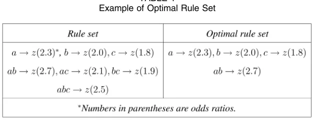
Each interestingness metric defines an optimal rule set and the above definition defines a family of optimal rule sets. We use the following example to elaborate the definition: Example 1.Let the interestingness metric be the odds ratio
(or). We have a rule set and its corresponding optimal rule set as shown in Table 1. Rules ac!zðor¼2:1Þ, bc!zðor¼1:9Þ, and abc!zðor¼2:5Þ are excluded since their odds ratios are smaller than those of their more general rules.
We provide another example to show the practical implication of an optimal rule set.
Example 2. When Interestingness is measured by an estimated accuracy of a rule, the optimal rule set is an optimal class association rule set [11]. Based on an ordered rule-based classification model, all rules ex-cluded by the optimal class rule set will not be used in building a classifier because they are less accurate and more complex than some rules in the optimal class association rule set covering the same data section. Therefore, a classifier built from the optimal class association rule set is identical to that from a class association rule set. In summary [11]: The optimal class association rule set is the minimum subset of rules with the same predictive power as the complete class association rule set. Further experimental proofs are reported in [10]. Classifiers built on the optimal class association rule sets are at least of the same accuracy as those from CBA [12] and C4.5 rules [15].
Building classifiers from optimal class association rule sets is significantly more efficient than building them from class association rule sets. First, mining optimal class association rule sets is significantly faster than mining class association rule sets. When the minimum support is low, mining class association rule sets may not be feasible. Second, an optimal class association rule set is significantly smaller than a class association rule set and, hence, building classifiers from the optimal class association rule set is more efficient.
In the next section, we discuss properties of the family of the optimal rule sets.
3
PROPERTIES OF
OPTIMAL
RULE
SETS
In this section, we discuss some properties of the family of optimal rule sets and their relationships with the non redundant rule set.
We start with some notation. Let Xbe a pattern where X6¼ ;and letcbe a class. P Xis a proper super pattern of P. P Q is a super pattern of P. P Q¼P and P QX¼P X when Q¼ ;. P QX is a proper super pattern of P. :c stands for a special class occurring in a record wherecdoes not occur, and, therefore, we havesuppð:cÞ ¼1suppðcÞ. Similarly for patternP:suppð:PÞ ¼ 1suppðPÞ.P:Xis a pattern with the following support: suppðP:XÞ ¼
suppðPÞ suppðP XÞ. Further, we have suppð:ðP XÞÞ ¼
suppð:P XÞ þ suppð:P:XÞ þsuppðP:XÞ.
Theorem 1 (Antimonotonic property). If suppðP X:cÞ ¼
suppðP:cÞ,1then ruleP X!cand all its more-specific rules will not occur in an optimal rule set defined by confidence, odds ratio, lift (interest or strength), gain, added-value, Klosgen, conviction, p-s (or leverage), Laplace, cosine, certainty factor, or Jaccard.
A proof is provided in the Appendix.
The practical implication of the above theorem is that once suppðP X:cÞ ¼suppðP:cÞ is observed, it is not necessary to search for more specific rules ofP X!c, for example,P QX!c. Those more specific rules will not be in an optimal rule set. RuleP X!cis removed since it is not in an optimal rule set either.
In the following, we consider two special cases of the above theorem:
Corollary 1 (Closure property). If suppðPÞ ¼suppðP XÞ, then ruleP X!cfor anycand all its more specific rules do not occur in an optimal rule set defined by confidence, odds ratio, lift (interest or strength), gain, added-value, Klosgen, conviction, p-s (or leverage), Laplace, cosine, certainty factor or Jaccard.
A proof is provided in the Appendix.
The practical implication of the above corollary is that, oncesuppðP XÞ ¼suppðPÞis observed, it is not necessary to search for rules withP QX as their antecedent for any Q. Those rules will not be in the optimal rule set.
[image:3.612.126.441.78.199.2]1. In this paper, we only discuss rules with a single class as the consequence, but this theorem holds for rules with a pattern as the consequence.
TABLE 1
The reason for naming the above corollary as the closure property is that it is closely related to closed pattern set mining [20].
Pattern Pc is closed if there exists no proper super
pattern XPc such that covðXÞ ¼covðPcÞ. Consider a
chain of patterns P P0P00 Pc, which satisfies covðPÞ ¼covðP0Þ ¼covðP00Þ ¼covðPcÞ.Pc is the closure of
patternsP,P0, andP00. A closed pattern is the same as its
closure. The support of a pattern is equivalent to that of its closure. In the above example, suppðPÞ ¼suppðP0Þ ¼
suppðP00Þ ¼suppðPcÞ. Further, a pattern Y is a proper generator of Y0 if Y0Y and covðY0Þ ¼covðYÞ hold. A pattern is a minimal generator if it has no proper generator. For example, P0 is a generator of P00 and Pc, and P is a
minimal generator ofPc if there exists noZP such that
covðPÞ ¼covðZÞ.
The closed pattern and minimal generator are two closely related concepts and the mining methods for both are very similar. The condition of Corollary 1 is the fundamental test for mining both patterns. For example, we have suppðPÞ ¼suppðP XÞ for any X ðPcnPÞ in the
above example. We illustrate this in Section 5. Usually, closed patterns are useful for producing all frequent patterns and minimal generators are useful for generating nonredundant rules.
Zaki [19] gave a general definition of nonredundant association rule sets. Here, we rephrase it in a simple form by constraining the consequence to c. Rule Y !c is redundant if there exists Y X such that covðYÞ ¼covðXÞ. suppðYÞ ¼suppðXÞ is the immediate result of covðYÞ ¼covðXÞ. For example, in the chain P P0P00Pc, all rules, such as P0!c, P00!c, and
Pc!c, are redundant since they have the same support
and interestingness as ruleP !cbut are more specific. A rule set is nonredundant if it includes all rules except redundant rules.
Theorem 2 (Relationship with the nonredundant rule set).
An optimal rule set is a subset of a nonredundant rule set.
A proof is provided in the appendix. We have another special case for Theorem 1.
Corollary 2 (Termination property).IfsuppðP:cÞ ¼0, then all more-specific rules of the rule P!c do not occur in an optimal rule set defined by confidence, odds ratio, lift (interest or strength), gain, added-value, Klosgen, conviction, p-s (or leverage), Laplace, cosine, certainty factor or Jaccard.
A proof is provided in the appendix.
The practical implication of the above corollary is that oncesuppðP:cÞ ¼0is observed, it is not necessary to search for more specific rules ofP !c. Those more-specific rules will not be in an optimal rule set. RuleP !cis kept since it may be in an optimal rule set.
Let us look at why it is called the termination property. Assume that the interestingness metric is confidence. If suppðP:cÞ ¼0, then rule confðP!cÞ ¼100%. None of its more specific rules improves this confidence and we stop going any further. The same is true for other interestingness metrics.
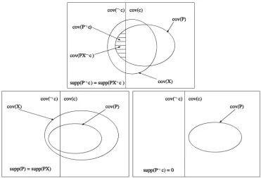
An illustrative comparison of conditions of Theorem 1 and Corollaries 1 and 2 is given in Fig. 1.
We use the following example to show how the Theorem 1 and its corollaries work.
[image:4.612.97.468.68.321.2]Example 3.We assumezis a class and do not assume the minimum support requirement in this example.
Fig. 1. Depictions of conditions of Theorem 1 and Corollaries 1 and 2. In each diagram, the left-hand rectangle stands for the set of records not containing the classc, and the right-hand rectangle stands for the set of records containing the classc. Ellipses denote the cover sets of patternsP
Usually, we have to consider all 15 candidate rules: a!z, b!z, c!z, d!z, ab!z, ac!z, ad!z, bc!z, bd!z, cd!z, abc!z, abd!z, acd!z, bcd!z, andabcd!z.
Sincesuppðab:zÞ ¼suppða:zÞ, according to Theorem 1, rule ab!z and all its more specific rules—abc!z, abd!z, andabcd!z—will not be in an optimal rule set. Similarly, both ruleac!zand rulebc!zand their more specific rules will not be in the optimal rule set.
Since suppðad:zÞ ¼0, all more specific rules of ad!z, e.g., abd!z,acd!z, andabcd!zwill not be in the optimal rule set. Similarly, all more specific rules ofcd!zwill not be in the optimal rule set.
Since suppðdÞ ¼suppðbdÞ, bd!c and all its more specific rules will not be in the optimal rule set.
Therefore, rules that are possible members of the optimal rule set are a!z,b!z,c!z,d!z,ad!z, and cd!z. This set of candidate rules is significantly smaller than the original 15 candidate rules.
4
AN
OPTIMAL
RULE
DISCOVERY
ALGORITHM
In this section, we first show how to use Theorem 1 and its corollaries for forward pruning. Then, we discuss a candi-date-presentation method for easy pruning. Sections 4.3 and 4.4 present the detailed implementation of forward pruning by Theorem 1 and its corollaries. The complete algorithm is presented in Section 4.5. After that, an illustrative example shows how the algorithm works.4.1 Basic Ideas and Forward Pruning
General-to-specific searching is very common in rule discovery. For example, C4.5rules, CN2, and Apriori employ this method.
When a heuristic search method is employed, we worry less about combinatorial explosion. However, when we conduct an optimal search, combinatorial explosion is a big problem.
We first look at how association rule discovery alleviates this problem. An association rule discovery algorithm prunes infrequent patterns forwardly. A pattern is frequent if its support is not less than the minimum support. A pattern is potentially frequent only if all its subpatterns are frequent and this antimonotonic property is used to limit the number of patterns to be searched. This is called forward pruning.
Optimal rule discovery makes use of Theorem 1 and its corollaries to forwardly prune rules.
We illustrate how Theorem 1 forwardly prunes rules that are not in an optimal set. Given a patternabcd, assume the target is fixed to z. We usually have to examine candidate rules a!z,b!z,. . . for one-patterns, ab!z, ac!z,. . . for two-patterns,abc!z,abd!z,. . . for three-patterns, and abcd!z for four-pattern. If we know suppða:zÞ ¼ suppðab:zÞ, then the theorem empowers us
to skip examining candidates, ab!z, abc!z, abd!z, and abcd!z because they are not in the optimal rule set anyway. Corollary 2 works in a similar way.
We show how Corollary 1 forwardly prunes rules that are not in an optimal rule set by using the above example. When the targets are not fixed tozbut include xand y too, the number of rule candidates is tripled. We list those including patternab in their antecedents as follows: ab!x,ab!y, ab!z,abc!x,abc!y,abc!z,abd!x,abd!y,abd!z, abcd!x,abcd!y, andabcd!z. If we know thatsuppðaÞ ¼
suppðabÞholds, then all candidates listed above are ignored according to Corollary 1. Corollary 1 prunes more candidates than Theorem 1, but its requirement is stricter.
4.2 Candidate Representation
To facilitate the implementation of forward pruning by Theorem 1 and its corollaries, we define a rule candidate as a pair of (pattern, target set), denoted by ðP ; CÞ. P is a pattern andCis a set of classes. In a relational data set, we haveP\C¼ ;. For example, letP¼abcandC¼xyz, and then ðP ; CÞ stands for three candidate rules: abc!x, abc!y, and abc!z. To remove a candidate rule, we simply remove a class from the target set. For example, candidate fabc; yzg stands for only two candidate rules, namely,abc!yandabc!z. When the target set is empty, the candidate stands for no rules.
The removal of classes from target setCis determined by Theorem 1 and its corollaries. For example, if we have suppðab:xÞ ¼suppðabc:xÞ, then, according to the theorem, ruleabc!xand all its more specific rules will not occur in the optimal rule set. x should be removed from the candidate set and the candidate becomes ðabc; yzÞ. If we knowsuppðabc:yÞ ¼0,yshould be removed from the target set according to Corollary 2, and the candidate becomes
ðabc; zÞ. Consider another candidate ðbcd; xyzÞ. If we have suppðbcdÞ ¼suppðcdÞ, then, according to Corollary 1, the target set of the candidate should be emptied and the candidate becomesðbcd;;Þ.
CandidateðP ;;Þshould be removed since no rules will be generated from it and its supercandidates. ðP0; C0Þ is
called a supercandidate ofðP ; CÞifP0P holds.
The existence of a candidate relies on two conditions: 1) PatternP is frequent, and 2) target setC is not empty.
4.3 Candidate Generator
For easy comparison, we present Candidate-gen for optimal rule-set discovery in a way similar to Apriori-gen. We call a candidate l-candidate if its pattern is an l-pattern. An l-candidateset includes alll-candidates.
Function:Candidate-gen // Combining
1) for each pair of candidatesðPl1s; CsÞ andðPl1t; CtÞin
anl-candidateset
2) insert candidateðPlþ1; CÞ in theðlþ1Þ-candidateset
wherePlþ1¼Pl1standC¼Cs\Ct
// Pruning 3) for allPlPlþ1
4) if candidateðPl; ClÞdoes not exist
5) then remove candidateðPlþ1; CÞand return
6) elseC¼C\Cl
7) if the target set ofðPlþ1; CÞis empty
First, we explain lines 1 and 2. Suppose that we have two candidates, ðabc; xyÞ and ðabd; yÞ. The new candidate is
ðabcd; yÞ. The intersection of target sets here and in line 6 is to ensure that removed classes from the target set of a candidate never appear in the target set of its super-candidates. The correctness is guaranteed by Theorem 1 and its corollaries since any class removal in the target set is determined by them.
Second, we explain lines 3 to 8. Suppose we have new candidate ðabcd; yÞ. It is the combination of ðabc; yÞ and
ðabd; yzÞ. We need to check if candidates identified by patternsfacdg andfbcdgexist. Suppose that they do exist and are ðacd; yÞ and ðbcd; xzÞ. After considering candidate
ðacd; yÞ; by line 7, the new candidate remains unchanged. After considering candidateðbcd; xzÞ, by line 7, the target set of the new candidate becomes empty because C¼
fyg \ fx; zg ¼ ;. The new candidate is then pruned.
4.4 More Pruning
We have a pruning process in candidate generation and will have another pruning process after counting the support of candidates. This is a key to making use of Theorem 1 and its corollaries for pruning. In the following algorithm,is the minimum support.
Function:Pruneðlþ1Þ
//lþ1is the new level where candidates are counted. 1) for each candidateðP ; CÞinðlþ1Þ-candidateset 2) for eachc2C
// test the frequency individually
3) ifsuppðP cÞ=suppðcÞ then removecfromC // test the satisfaction of Corollary 2
4) else ifsuppðP:cÞ ¼0then markcterminated 5) ifCis empty then remove candidateðP ; CÞand return 6) for eachl-levelsubsetP0P
// test the satisfaction of Corollary 1 7) ifsuppðPÞ ¼suppðP0Þthen emptyC
// test the satisfaction of Theorem 1 8) else ifsuppðP:cÞ ¼suppðP0:cÞthen
removecfromC
9) ifCis empty then remove candidateðP ; CÞ
We prune candidates from two aspects, the infrequency of the pattern and the emptiness of the target set.
Here, we consider a local support instead of the global support. Because of the possible skewed distributions of classes, a single global support is not suitable for a variant rule targeting different classes. Many applications have adopted local support in spite of using different names, such as coverage in [3]. The local support of rule P!cis defined as suppðPcÞ=suppðcÞ. The local support is the support in the data subset containing c. It is also called the recall of rule P !c. We prefer local support since it observes the antimonotonic property of the support. When we make use of local support, infrequent candidate rules are removed one by one, as in line 3.
We are aware of two variants of the forward pruning by Theorem 1 and Corollary 2. One is that ruleP X!cand all its more-specific rules are not in an optimal rule set as in Theorem 1. In this case, we just removecfrom the target set. Another is that all more specific rules of ruleP !care not
in an optimal rule set except ruleP !c, as in Corollary 2. In this case, we cannot removecsince we may lose ruleP !c. We design a special statue for this situation, namely, termination of targetc.
Definition 4.Targetc2Cis terminated in candidateðP ; CÞif
suppðP cÞ ¼0.
Terminatedcis removed after the rule forming in line 9 of the ORD algorithm.
Line 4 of the Prune function is a direct application of Corollary 2. Target cis marked as terminated and will be removed after a rule is formed. Oncecis removed fromC, all more-specific rules of P !c will be removed in the following rule-candidate generation.
Line 7 of the Prune function is a direct result of Corollary 1. All classes inC are removed and, as a result, candidateðP ; CÞis removed. No supercandidates ofðP ; CÞ
will be formed in the following rule-candidate generation. Line 8 of the Prune function is a direct utilization of Theorem 1. Targetcis removed and, therefore, ruleP !c and all its more-specific rules are removed in the following candidate generation.
All candidates with an empty target set are removed in lines 5 and 9 to ensure their supercandidates are pruned in the following candidate generation.
4.5 ORD Algorithm
Now, we are able to present our algorithm for optimal rule discovery, abbreviated ORD. In this algorithm, any inter-estingness metric discussed in Section 3 can be used as a rule-selection criterion and the output rule set is an optimal rule set defined by the interestingness metric. It differs from association rule discovery in that it does not form rules from the set of all frequent patterns, but generates rules using partial frequent patterns.
Algorithm 1ORD: Optimal Rule Discovery
Input: a data setD, the minimum local supportand the
minimum interestingnessby a metric.
Output: an optimal rule setRdefined by an interestingness metric.
1) SetR¼ ;
2) Count support of one-patterns by arrays 3) Build one-candidate sets
4) Form and add rules toR 5) Generate two-candidate set
6) While new candidate set is not empty
7) Count support of patterns for new candidates 8) Prune candidates in the new candidate set 9) Form rules and add optimal rules toR 10) Generate next-level candidate set 11) Return the rule setR
The above algorithm is self-explanatory and its two main functions have been discussed in the previous sections.
4.6 An Illustrative Example
We provide an example to show how the ORD algorithm works in this section.
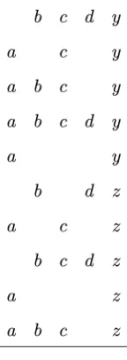
[image:7.612.30.271.71.183.2]Example 4.In the following data set,yandzare classes. We do not assume the minimum support constraint. All candidates generated by the ORD algorithm are listed in Fig. 2.
The first-level candidates are used to prune the second-level candidates. z is removed in candidate
ðad; yzÞ by line 3 in Function Prune due to suppðadzÞ ¼0. y in candidate ðad; yzÞ is terminated by line 4 in Function Prune because ofsuppðad:yÞ ¼0. Both y and z are removed in candidateðbd; yzÞ by line 7 in Function Prune since suppðbdÞ ¼suppðdÞ holds. z in
candidate ðbc; yzÞ and ðcd; yzÞ is removed by Line 8 in Function Prune because both suppðbc:zÞ ¼suppðb:zÞ
andsuppðcd:zÞ ¼suppðd:zÞhold.
After rules have been formed, candidatesðad;;Þand
ðbd;;Þare removed. As a result, all their supercandidates, such as ðabd;;Þ, ðacd;;Þ, and ðbcd;;Þ, will not be generated according to lines 4 and 5 in Function Candidate-gen.
Candidateðabc; yzÞis generated by combining candi-dates ðab; yzÞ and ðac; yzÞ according to lines 1 and 2 in Function Candidate-gen. z is then pruned by line 7 in Function Candidate-gen using its subcandidateðbc; yÞ.y in candidate ðabc; yÞ is removed by line 8 in Function Prune due to suppðabc:yÞ ¼suppðab:yÞ. Subsequently, candidateðabc;;Þis removed.
In the rule-forming procedure, rules are formed by a user-specified interestingness metric. No matter what metric discussed in Section 3 is used, the set of candidates is identical. Only the output rule set differs.
5
SUPPORT
PRUNING, CLOSURE
PRUNING AND
OPTIMALITY
PRUNING
In this section, we discuss support pruning, closure pruning, and optimality pruning and then characterize relationships among them. This clarifies the efficiency improvement of optimal rule discovery over association rule discovery and nonredundant rule discovery.
[image:7.612.121.193.321.524.2]First, look at the support pruning of the following data set:
Fig. 3 shows support pruning using the minimum support of 0.2. We see that the removal of e in Level 1 equals the removal of 15 patterns in subsequent levels, such asae,be,. . .,abe,ace,. . .,abce,abde,. . ., andabcde.
[image:7.612.139.427.623.741.2]Support pruning works effectively when the underlying data set is sparse or the minimum support is high. Fig. 2. All candidates searched in Example 4. A class crossed is
removed and a class boxed is terminated.
However, it does not work well on dense data sets or when the minimum support is low.
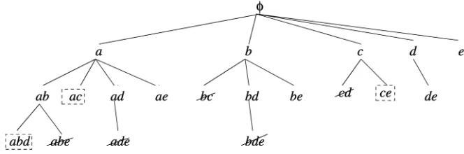
[image:8.612.115.447.70.180.2]Look at the closure pruning by the following data set:
Fig. 4. shows the closure pruning. There is no minimum support requirement.
As discussed in Section 3, Corollary 1 summarizes the closure pruning. Each pattern in a box is terminated because the support of its superpatterns equals that of itself. If the final goal is to find minimal generators, all candidates are left as they are in Fig. 4. If the the final goal is to find closed patterns, the number of candidates remains unchanged, but patterns in some candidates are extended. For example, ac is terminated due to suppðacÞ ¼suppðcÞ
and, as a result, all occurrences ofcwill be replaced byac. Similarly, all occurrences of c are further replaced by ce because of the termination of ce by suppðceÞ ¼suppðcÞ. Patternaceis the only closed pattern left out in Fig. 4, and other minimal generators are closed patterns too. Closed patterns can be discovered in the same search tree finding minimal generators. Therefore, both closed-pattern mining and minimal-generator mining search for the same number of candidates and make use of the closure pruning strategy. Closure pruning works effectively when the underlying data set is dense or the minimum support is low. We use an example to elaborate the first point. Assume that a dense data set contains five identical recordsfa; b; c; d; eg. Closed-pattern mining will stop at Level 2 after searching for 15 candidates. In contrast, frequent-pattern mining will continue all the way to Level 5 and search for 251 candidates. We present the following justification for the second point:suppðP XÞ ¼suppðPÞmeanscovðPÞ covðXÞ. WhencovðXÞremains unchanged, patternPwith a smaller covðPÞ is more probable to satisfy covðPÞ covðXÞ than with a larger covðPÞ.
The above two pruning strategies are complementary. How does the ORD algorithm use them in an effective way? Let us look at the following data set concatenating the above two data sets.zis the target for rules. Fig. 5 shows the optimality pruning with the minimum local support of 0.2 in the data subset containingz.
The candidate set searched by optimal rule discovery is the intersection of the candidate set (frequent patterns) for association rule discovery in z data subset and the candidate set (minimal generators) for nonredundant rule discovery in:zdata subset. The crucial point is that both have to perform simultaneously. Both association rule discovery and nonredundant rule discovery search for more candidates than optimal rule discovery.
Now, we have an insight understanding of optimality pruning as stated in Theorem 1. It makes use of the closure pruning strategy. Comparing Corollary 1 with Theorem 1, we find that Theorem 1 states Corollary 1 in the data subset excludingc.
[image:8.612.362.461.216.414.2]Fig. 4. Closure pruning for mining minimal generators on data set B. Patterns crossed are nonexisting and patterns boxed are terminated
[image:8.612.300.530.621.727.2]6
EXPERIMENTAL
RESULTS
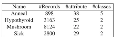
In this section, we empirically evaluate the computational complexity of optimal rule discovery in comparison with association rule discovery and nonredundant association rule discovery on four data sets from UCML repository [4] described in Table 2. The efficiency of optimal rule discovery is its effective optimality pruning. We show that optimality pruning significantly reduces candidates for searching.
The efficiency of an algorithm significantly depends on the data structure and implementation. For example, association rule discovery has various implementations. All are based on support pruning strategy, but their execution times vary. Theoretically, their computational complexities are the same since they all search for all frequent patterns. Their efficiencies vary since they employ different data structures and counting schemes. There are a number of implementations for association rule discovery and we are unable to compare with them individually by execution time.
However, the computational complexity improvement is fundamental and the implementation only accelerates the improvement. An empirical estimation of the complexity for a rule-discovery algorithm is the number of candidates it searches. In this paper, we compare the searched candidates for association rule discovery, for nonredundant association rule discovery, and for optimal rule discovery. An associa-tion-discovery algorithm searches for all frequent patterns and a nonredundant rule-discovery algorithm searches for all frequent minimal generators (equivalently, all frequent closed patterns). We compare the number of candidates for the ORD algorithm with the number of frequent patterns and the number of frequent minimal generators. This comparison is independent of the implementation.
In this experiment, we employ the local support as defined in Section 4.4, which is a ratio for an individual class. A pattern is frequent if it is frequent in at least one class. All frequent patterns are stored in the prefix tree.
The experiment was conducted on a 1 GHz CPU computer with 2 Gbytes memory running Linux. We search for rules containing up to eight attribute-value pairs. We do not specify the type of optimal rule set since the same candidate set generates an optimal rule set defined by any interestingness metric discussed in Section 3.
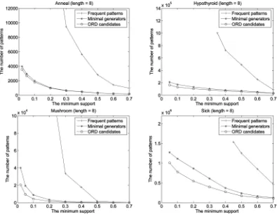
Fig. 6 shows the searched candidates by the ORD algorithm in comparison with the number of frequent patterns and the number of frequent minimal generators. The set of ORD candidates is a very small subset of frequent patterns and a subset of frequent minimal generators. This
trend is more evident when the minimum support is low. This shows that optimal rule discovery has significantly less computational complexity than association rule discovery, and less computational complexity than nonredundant association rule discovery.
In comparison with optimal rule discovery and non redundant rule discovery, association rule discovery is very inefficient in data sets such as were used in this experiment. The efficiency of association rule discovery deteriorates dramatically when the minimum support is low. Optimal rule discovery is more efficient than nonredundant associa-tion rule discovery. Though differences between candidate numbers of nonredundant association rule discovery and optimal rule discovery are squashed in Fig. 6 by the large number of frequent patterns, the discrepancies are still clear in data sets Mushrooms and Sick.
7
CONCLUSIONS
In this paper, we discussed a family of optimal rule sets, the properties for their efficient discovery, and their relation-ships with the nonredundant rule sets. The family of optimal rule sets supports a simple antimonotonic property and an optimal rule set is a subset of a nonredundant rule set. We presented the ORD algorithm for mining optimal rule sets and evaluated its computational complexity on some data sets in comparison with the association rule discovery and nonredundant association rule discovery. The computational complexity of optimal rule discovery is significantly lower than that of association rule discovery and lower than that of nonredundant association rule discovery. We discussed the relationship of optimal prun-ing with support prunprun-ing and closure prunprun-ing and we concluded that optimality pruning makes use of both support and closure pruning strategies simultaneously on two disjointed data sets.
Optimal rule discovery is efficient and works well with low or no minimum support constraint. It generates optimal rule sets for a number of interestingness metrics. Therefore, it is a great alternative for association rule discovery.
APPENDIX
In this appendix, we provide proofs for Theorems 1 and 2, and Corollaries 1 and 2.
Theorem 1 (antimonotonic property). If suppðP X:cÞ ¼
suppðP:cÞ, then rulesuppP X!cand all its more specific rules will not occur in an optimal rule set defined by confidence, odds ratio, lift (interest or strength), gain, added-value, Klosgen, conviction, p-s (or leverage), Laplace, cosine, certainty factor, or Jaccard.
Proof.In the proof, we show
InterestingnessðP QX!cÞ InterestingnessðP Q!cÞ:
Therefore, ruleðP X!cÞ(whenQ¼ ;) and all its more specific rules, for example,P QX!c(whenQ6¼ ;), will not occur in the optimal rule set.
The only case for the condition suppðP X:cÞ ¼
[image:9.612.59.242.96.156.2]suppðP:cÞ holding is that covðP:cÞ covðX:cÞ. We TABLE 2
then deduce that covðP Q:cÞ covðQX:cÞ for any Q. Consequently, suppðP QX:cÞ ¼suppðP Q:cÞ holds for anyQ.
For the confidence case, consider fðyÞ ¼y=ðyþÞ
monotonically increases withywhen constant >0and suppðP QÞ suppðP QXÞ>0:
confðPQ!cÞ ¼suppðP QcÞ
suppðP QÞ
¼ suppðP QcÞ
suppðP QcÞ þsuppðP Q:cÞ
¼ suppðP QcÞ
suppðP QcÞ þsuppðP QX:cÞ
suppðPQXcÞ
suppðP QXcÞ þsuppðP QX:cÞ ¼confðP QX!cÞ:
We then prove the odds ratio case. Odds ratio is a classic statistical metric to measure the association between events. Consider fðyÞ ¼y=ðyÞ monotoni-cally increases with y when constant >0 and suppðP QÞ suppðP QXÞ>0:
orðP Q!cÞ ¼ suppðP QcÞsuppð:ðP QÞ:cÞ
suppðð:ðP QÞcÞsuppðP Q:cÞ
¼suppðP QcÞðsuppð:cÞ suppðP Q:cÞÞ ðsuppðcÞ suppðP QcÞÞsuppðP Q:cÞ
¼suppðP QcÞðsuppð:cÞ suppðP QX:cÞÞ ðsuppðcÞ suppðP QcÞÞsuppðP QX:cÞ
¼ suppðP QcÞsuppð:ðP QXÞ:cÞ
ðsuppðcÞ suppðP QcÞÞsuppðP QX:cÞ
suppðP QXcÞsuppð:ðP QXÞ:cÞ ðsuppðcÞ suppðP QXcÞÞsuppðP QX:cÞ
¼suppðP QXcÞsuppð:ðP QXÞ:cÞ
suppð:ðPQXÞcÞsuppðPQX:cÞ ¼orðP QX!cÞ:
Lift, also known as interest [5] or strength [8], is a widely used metric for ranking the interestingness of association rules. It has been used in IBM Intelligent Miner. We make use of the previous results,confðP Q!
cÞ confðP QX!cÞ, in the following proof:
liftðP Q!cÞ ¼ suppðP QcÞ
suppðP QÞsuppðcÞ
¼confðP Q!cÞ
suppðcÞ
confðP QX!cÞ
[image:10.612.87.482.71.376.2]suppðcÞ ¼liftðP QX!cÞ:
Gain [9] is an alternative for confidence. Fraction is a constant in interval ð0;1Þ and only rules obtaining positive gain are interesting. We use confðP Q!cÞ
confðP QX!cÞ> in the following proof:
gainðP Q!cÞ ¼suppðP QcÞ suppðP QÞ ¼ ðconfðP Q!cÞ ÞsuppðP QÞ
ðconfðP QX!cÞ ÞsuppðP QXÞ
¼gainðP QX!cÞ:
The proofs for metrics added-value,
addedvalueðP!cÞ ¼confðP!cÞ suppðcÞ;
and Klosgen,
KlosgenðP !cÞ ¼pffiffiffiffiffiffiffiffiffiffiffiffiffiffiffiffiffiffiffiffisuppðP cÞðconfðP!cÞ suppðcÞÞ;
are very straightforward and, hence, we omit them here. Conviction [5] is used to measure deviations from independence by considering outside negation:
convictionðP Q!cÞ ¼suppðP QÞsuppð:cÞ
suppðP Q:cÞ
¼suppðP QÞð1suppðcÞÞ
suppðP QÞ suppðP QcÞ
¼ 1suppðcÞ
1confðP Q!cÞ
1suppðcÞ
1confðP QX!cÞ ¼convictionðPQX!cÞ:
P-s metric (or leverage), psðP!cÞ ¼suppðP cÞ
suppðPÞsuppðcÞ, is a classic interestingness metric for rules proposed by Piatesky-Shaprio [14]. The proof for it is very similar to that of gain and hence we omit it.
Laplace [6], [17] accuracy is a metric for classifica-tion rules. jDj is the number of transactions in D and k is the number of classes. In classification problems, k2 and, usually, confðP QX!cÞ 0:5. Therefore, k confðP QX!cÞ 1 holds. Function fðyÞ ¼ ðjDj þyÞ=
ðjDj þkyÞ monotonically decreases withy when k > 1 and 1=suppðP QXÞ 1=suppðP QÞ.
LaplaceðP Q!cÞ ¼suppðP QcÞjDj þ1
suppðP QÞjDj þk
¼confðP Q!cÞjDj þ1=suppðPQÞ jDj þk=suppðP QÞ
confðP QX!cÞjDj þ1=suppðP QÞ jDj þk=suppðP QÞ
confðP QX!cÞjDj þ1=suppðP QXÞ jDj þk=suppðP QXÞ ¼LaplaceðP QX!cÞ:
The proofs for the following two metrics are straight-forward and, hence, we omit them:
CosineðP !cÞ ¼suppðP cÞ=ðpffiffiffiffiffiffiffiffiffiffiffiffiffiffiffiffiffiffiffiffiffiffiffiffiffiffiffiffiffiffiffiffiffisuppðPÞsuppðcÞÞ
and
CertaintyfactorðP !cÞ ¼
ðconfðP !cÞ suppðcÞÞ=ð1suppðcÞÞ:
Finally, we prove the metric of Jaccard.
JaccardðP Q!cÞ
¼ suppðP QcÞ
suppðP QÞ þsuppðcÞ suppðP QcÞ
¼ confðP Q!cÞ
1þsuppðcÞ=suppðP QÞ confðP Q!cÞ
confðP Q!cÞ
1þsuppðcÞ=suppðP QXÞ confðP Q!cÞ
confðP QX!cÞ
1þsuppðcÞ=suppðP QXÞ confðP QX!cÞ ¼JaccardðP QX!cÞ:
The theorem has been proved. tu
Corollary 1 (Closure property). If suppðPÞ ¼suppðP XÞ, then ruleP X!cfor anycand all its more-specific rules do not occur in an optimal rule set defined by confidence, odds ratio, lift (interest or strength), gain, added-value, Klosgen, conviction, p-s (or leverage), Laplace, cosine, certainty factor, or Jaccard.
P r o o f . I f suppðPÞ ¼suppðP XÞ, t h e n suppðP:cÞ ¼
suppðP X:cÞ holds for any c. Therefore, this Corollary is proved immediately by Theorem 1. tu
Corollary 2 (Termination property).IfsuppðP:cÞ ¼0, then all more-specific rules of the rule P!c do not occur in an optimal rule set defined by confidence, odds ratio, lift (interest or strength), gain, added-value, Klosgen, conviction, p-s (or leverage), Laplace, cosine, certainty factor, or Jaccard.
Proof.IfsuppðP:cÞ ¼0, thensuppðP X:cÞ ¼suppðP:cÞ ¼0 holds for any X. Therefore, this corollary is proved
immediately by Theorem 1. tu
Theorem 2 (Relationship with the nonredundant rule set).
An optimal rule set is a subset of a nonredundant rule set.
Proof. Suppose that we have suppðPÞ ¼suppðP XÞ and there is noP0Psuch thatsuppðPÞ ¼suppðP0Þ. The rule P X!c for any c is redundant. It will not be in an optimal rule set either, according to Corollary 1.
Suppose thatsuppðPÞ ¼suppðP XÞ and there isP0
P such that suppðPÞ ¼suppðP0Þ. We always have
suppðP0Þ ¼ suppðP0YÞ for Y ðP XnP0Þ. Rules P !c and P X!c are redundant. They will not be in an optimal rule set either, according to Corollary 1.
Further, many nonredundant rules are pruned by Theorem 1.
Therefore, an optimal rule set is a subset of a
nonredundant rule set. tu
ACKNOWLEDGMENTS
REFERENCES
[1] R. Agrawal, T. Imielinski, and A. Swami, “Mining Associations Between Sets of Items in Massive Databases,”Proc. ACM SIGMOD Int’l Conf. Management of Data,pp. 207-216, 1993.
[2] R. Bayardo and R. Agrawal, “Mining the Most Interesting Rules,”
Proc. Fifth ACM SIGKDD Int’l Conf Knowledge Discovery and Data Mining,pp. 145-154, 1999.
[3] R. Bayardo, R. Agrawal, and D. Gunopulos, “Constraint-Based Rule Mining in Large, Dense Databases,” Data Mining and Knowledge Discovery J.,vol. 4, nos. 2/3, pp. 217-240, 2000.
[4] E.K.C. Blake and C.J. Merz, UCI Repository of Machine Learning Databases, http://www.ics.uci . edu/~mlearn/MLRepository. html, 1998.
[5] S. Brin, R. Motwani, J.D. Ullman, and S. Tsur, “Dynamic Itemset Counting and Implication Rules for Market Basket Data,” Proc. ACM SIGMOD Int’l Conf. Management of Data, vol. 26, no. 2, pp. 255-264, 1997.
[6] P. Clark and R. Boswell, “Rule Induction with CN2: Some Recent Improvements in Machine Learning,“Proc. Fifth European Working Session Learning (EWSL ’91),pp. 151-163, 1991
[7] W.W. Cohen, “Fast, Effective Rule Induction,”Proc. 12th Int’l Conf. Machine Learning (ICML),pp. 115-123, 1995.
[8] V. Dhar and A. Tuzhilin, ”Abstract-Driven Pattern Discovery in Databases,“ IEEE Trans. Knowledge and Data Eng., vol. 5, no. 6, pp. 926-938, Dec. 1993.
[9] T. Fukuda, Y. Morimoto, S. Morishita, and T. Tokuyama, “Data Mining Using Two-Dimensional Optimized Association Rules: Scheme, Algorithms, and Visualization,”Proc. ACM SIGMOD Int’l Conf. Management of Data,pp. 13-23, 1996.
[10] H. Hu and J. Li, “Using Association Rules to Make Rule-Based Classifiers Robust,”Proc. 16th Australasian Database Conf. (ADC),
pp. 47-52, 2005.
[11] J. Li, H. Shen, and R. Topor, “Mining the Optimal Class Association Rule Set,” Knowledge-Based Systems, vol. 15, no. 7, pp. 399-405, 2002.
[12] B. Liu, W. Hsu, and Y. Ma, “Integrating Classification and Association Rule Mining,” Proc. Fourth Int’l Conf. Knowledge Discovery and Data Mining (KDD ’98),pp. 27-31, 1998.
[13] E. Omiecinski, “Alternative Interest Measures for Mining Associa-tions in Databases,”IEEE Trans. Knowledge and Data Eng.,vol. 15, no. 1, pp. 57-69, Jan. 2003.
[14] G. Piatetsky-Shapiro, “Discovery, Analysis and Presentation of Strong Rules,” Knowledge Discovery in Databases, G. Piatetsky-Shapiro, ed., pp. 229-248. Menlo Park, Calif.: AAAI Press/The MIT Press, 1991.
[15] J.R. Quinlan, C4.5: Programs for Machine Learning. San Mateo, Calif.: Morgan Kaufmann, 1993.
[16] P. Tan, V. Kumar, and J. Srivastava, “Selecting the Right Objective Measure for Association Analysis,” Information Systems,vol. 29, no. 4, pp. 293-313, 2004.
[17] G.I. Webb, “OPUS: An Efficient Admissible Algorithm for Unordered Search,” J. Artificial Intelligence Research, vol. 3, pp. 431-465, 1995.
[18] G.I. Webb and S. Zhang, “K-Optimal Rule Discovery,” Data Mining and Knowledge Discovery J.,vol. 10, no. 1, pp. 39-79, 2005.
[19] M.J. Zaki, “Mining Non-Redundant Association Rules,” Data Mining and Knowledge Discovery J.vol. 9, pp. 223-248, 2004.
[20] M.J. Zaki and C.J. Hsiao, “Charm: An Efficient Algorithm for Closed Association Rule Mining,” Proc. SIAM Int’l Conf. Data Mining,2002.
Jiuyong Lireceived the BSc degree in physics and MPhil degree in electronic engineering from Yunna University in China in 1987 and 1998 respectively, and received the PhD degree in computer science from Griffith University in Australia in 2002. He is currently a lecturer at the University of Southern Queensland in Aus-tralia. His main research interests are in rule discovery and health informatics.