A comparative study of velocity obstacle approaches for multi-agent systems

This is a repository copy of

A comparative study of velocity obstacle approaches for

multi-agent systems

.

White Rose Research Online URL for this paper:

http://eprints.whiterose.ac.uk/135915/

Version: Accepted Version

Proceedings Paper:

Douthwaite, J.A. orcid.org/0000-0002-7149-0372, Zhao, S. and Mihaylova, L.S.

orcid.org/0000-0001-5856-2223 (2018) A comparative study of velocity obstacle

approaches for multi-agent systems. In: Proceedings of 2018 UKACC 12th International

Conference on Control (CONTROL). Control 2018: The 12th International UKACC

Conference on Control, 05-07 Sep 2018, Sheffield, UK. IEEE , pp. 289-294. ISBN

978-1-5386-2864-5

https://doi.org/10.1109/CONTROL.2018.8516848

© 2018 IEEE. Personal use of this material is permitted. Permission from IEEE must be

obtained for all other users, including reprinting/ republishing this material for advertising or

promotional purposes, creating new collective works for resale or redistribution to servers

or lists, or reuse of any copyrighted components of this work in other works. Reproduced

in accordance with the publisher's self-archiving policy.

[email protected]

Reuse

Items deposited in White Rose Research Online are protected by copyright, with all rights reserved unless indicated otherwise. They may be downloaded and/or printed for private study, or other acts as permitted by national copyright laws. The publisher or other rights holders may allow further reproduction and re-use of the full text version. This is indicated by the licence information on the White Rose Research Online record for the item.

Takedown

If you consider content in White Rose Research Online to be in breach of UK law, please notify us by

A Comparative Study of Velocity Obstacle Approaches for Multi-Agent

Systems

James A. Douthwaite, Shiyu Zhao and Lyudmila S. Mihaylova

Abstract— This paper presents a critical analysis of some of the most promising approaches aimed at geometrically generating reactive avoidance trajectories for multi-agent systems. Several evaluation scenarios are proposed that include both sensor uncertainty and increasing difficulty. An intensive 1000 cycle Monte Carlo analysis is used to assess the performance of the selected algorithms under the presented conditions. The Optimal Reciprocal Collision Avoidance (ORCA) method was shown to demonstrate the most scalable computation times and collision likelihood in the presented scenarios. The respective features and limitations of the algorithms are discussed and presented through examples.

Index Terms— Collision avoidance, multi-agent systems, veloc-ity obstacles, VO, RVO, HRVO, OCRA

I. INTRODUCTION

Collision avoidance is a subject that has seen an increasing interest over the last decade with the growth of domestic and commercial robotics. Multi-agent systems are now required to navigate increasingly crowded and dynamic environments, of-ten where inter-agent communication is unreliable. In addition to this, in systems composed of numerous physical agents, agents must be able to generate trajectories in order to avoid other agents and obstacles in the field.

Two principle classifications of reactive avoidance tech-niques can be drawn from the literature: 1) Cooperative, 2) Non-cooperative. In both cases assumptions are made based on the availability of the obstacle telemetry. Cooperative avoid-ance algorithms operate on the assumption of a unilateral communication system with explicit communication between each agent and obstacle. Non-cooperative approaches however, rely on obstacle telemetry sensed through an on board tracking system. While typically multi-agent systems rely on com-municated information about its neighbours, we examine the scenario where agents are tasked with locally computing their trajectories to achieve a desired way-point. This is synonymous to scenarios where inadequate information is communicated or lost. This reduces the agent trajectory generation to a localised Sense, Detect and Avoidance (SDA) problem [1].

Previous approaches to solving the SDA problem in-clude probabilistic modelling [2], conflict resolution interval and agent trajectory optimisation [3]–[6]. More classical ap-proaches include designed potential fields as seen in [7] and

The authors gratefully acknowledge the support from the UK EPSRC under grant number EP/M506618/1. James A. Douthwaite, Shiyu Zhao and Lyudmila S. Mihaylova are with the Department of Automatic Control and Systems Engineering, The University of Sheffield, UK.jadouthwaite1, zhao, [email protected].

OpenMAS MatlabR _{simulation environment available at}

https://github.com/douthwja01/OpenMAS

numerous geometry based avoidance techniques [8], [9]. The concept of the Collision Cone and the Velocity Obstacle is introduced in [8], defining geometric regions as constraints on the agents feasible velocities at timetk+1. Presentation of the

collision scenario geometrically, given no prior knowledge or predictions, allows a resolution velocity to be found quickly and with minimal obstacle information.

Iterations of the Velocity Obstacle concept include the Re-ciprocal Velocity Obstacle [10], [11], which has been shown to reduce the trajectory oscillation by considering the reactive nature of avoiding agents. Variable acceleration obstacles are addressed under the notion ofAcceleration Velocity Obstacles

in [12]. Hybrid-Reciprocal Velocity Obstacle are introduced in an effort to eliminate direction ambiguity in [13] and eliminate the phenomenon known as the reciprocal dance. Despite producing smoother trajectories, the HRVO is not capable of guaranteeing that trajectories will be smooth. A method proposed to address this is the Optimal Reciprocal Collision Avoidance method, by adopting the concept of half-planes as linear constraints [14]. Similar techniques demon-strate consideration for non-linear obstacle motion, proposed in [15], with the addition of kinematic constraints in the

Kinematic Velocity Obstacles (KVO) in [16]. Although these approaches have been widely used in multi-agent systems such as pedestrian modelling and small robotic systems, they face challenges in symmetric scenarios where a phenomenon known as Dead-lockcan occur.

This paper presents an in depth analysis of the most promis-ing models and approaches for multi-agent collision avoidance. These approaches are studied over a range of scenarios with varying levels of difficulty and obstacle numbers. Through an intensive Monte Carlo analysis the pros and cons of these algo-rithms are demonstrated and discussed. These are evaluated in the light of a minimum separation distance and computation time, and can be applied both to unmanned aerial vehicles and air traffic control. Two dimensional collision avoidance is considered, although the extension to the three dimensional case is natural.

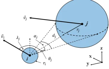
Fig. 1. A description of the adopted sensor model defining the spherical position of obstaclej, at timek, as its position in the azimuthdj,θjandλj.

in Section VI.

II. PROBLEMDESCRIPTION

We begin by considering an interaction between two agents,

i and j, respectively. Both agents are moving through two dimensional (2D) Cartesian space. The agents velocities are denoted by ~vi ∈ R3×1 and ~vj ∈ R3×1, with representative

radii ri andrj, respectively. Agenticonsiders agentj as both

a collaborator and an obstacle to be avoided. The position of agentiat timetk+1is defined as~pi,k+1=~pi,k+∆t·~vi,kwhere

∆tis the sampling rate. We define a maximum speed constraint

vmax to limit the velocities available to the avoidance routine;

represented simply as |~vi|<=vmax. A. Sensor Model

We assume that each agent is able to make its own observa-tions of its surrounding using an on board camera and range finder. The resulting measurements represent the spherical position of agentjin the form of an elevation, azimuth angle, range and width, denoted by θj ∈ [−π, π], λj ∈ [−π, π],

dj ∈[0, dmax] andαj ∈ [−π, π] respectively. The parameter

dmax is used here to describe the maximum visual range of

agent i. Agent i observes agent j in its body axes as seen in Figure 1 [3].

For the context of this paper we assume avoidance is to be carried out at constant altitude. Agentimeasures the spherical position,θj,k, λj,k, dj,k, and widthαj,k in the body axes ofi.

The agent then computes its equivalent 2D Cartesian position

~

pj,k = [xj,k, yj,k]T and radius estimate rj,k at time k. The

Cartesian velocity of the obstacle is then be calculated from successive position samples ~vi,k = ∆1t(pj,k −pj,k−1). The

relative state of obstacle j, at time tk, is then defined as

Xj,k = [pj,k, vj,k, rj]T. The agents are otherwise assumed

capable of retaining a set of states that correspond to all obstacles with in the agent’s visual horizon dmax.

III. VELOCITYOBSTACLEMETHODS

A. The Velocity Obstacle

The concept of the Velocity Obstacle (VO), based on the geometric assembly of the Collision Cone (CC), was first presented in [8]. Obstacles are observed in the agents local horizontal plane (XY) as their planar cross-section centred at

Fig. 2. The Velocity ObstacleV Oj(shaded in dark grey) from the initial CCij. Here theV Ojdefined in the configuration space ofi, from the relative

positionλij, configuration radiusrc=ri+rjand velocity~vj.

~

pjas seen in Figure 2. Here, the collision cone for obstaclejis

defined asCCijfrom the geometric properties of the obstacles

relative position~λij, configuration radius rc and velocity~vj.

Velocities that will bring about collision with obstacle j

are then be represented in the velocity space by translating

CCij by~vj via the Minkowski sum: V Oij =CCij ⊕~vj. In

the consideration of multiple obstacles, the union of multiple

V O1:nis taken. Agent velocities are therefore considered valid

if ~vi,k+1 6∈V Ok =∪nj=1V Oj,k [8]. Velocities satisfying this

constraint describe a collision free trajectory for agentiin the presence of obstaclesV Oj=1:n for time tk.

In practice, oscillatory trajectories are often observed in instances where two agents attempt to resolve a conflict with one another using theVO method. This often propagates until the point of collision occurs; as the two agents repeatedly resolve velocities~vi,k+1that imply a new conflict attk+1[10].

Obstacles that are static, or moving with constant velocity can otherwise be handled using the VOapproach.

B. The Reciprocal Velocity Obstacle

An iteration of the conventional VO method, termed the

Reciprocal Velocity Obstacle (RVO) [10], attempts to consider the reciprocal motion of the second decision making agent j

in order to produce smoother avoidance trajectories. The agent generates aVOwith an apex augmented by the average of the two object velocities ~vi,k+1 6∈ CCij⊕(~vi,k+~vj,k)/2. This

concept effectively allows the agent to mediate its correction trajectory ~vi,k+1 in accordance with~vj. At timetk, theRVO

contains represents the region of velocities for i that are the average of both the velocity of agent i and the velocity of obstaclej.

Fig. 3. The construction of the Reciprocal Velocity Obstacle (RV Oj) by

averaging the velocities of the agent~viand obstacle~vj.

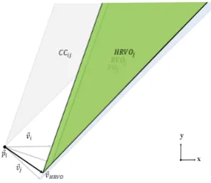
Fig. 4. The relation of the Hybrid Reciprocal Velocity obstacleHRVOto the initialV Ojand theRV Ojfor a given obstacleB.

C. The Hybrid Reciprocal Velocity Obstacle

An advancement on the VO problem has been proposed to negate the causes of reciprocal dance by augmenting the VO

and RVO regions. The Hybrid Reciprocal Velocity Obstacle (HRVO), shown in Figure 4, alters the apex of the HRVO in order to example different behaviour depending on the relative motion of the obstacle~vj.

The centreline of theV OjandRV Ojare collinear in nature,

therefore if the obstacle is moving right, the agent should resolve a trajectory~vi,k+1 to pass the obstacle on the left and

vice versa. Failure to do so brings about the phenomena of the

Reciprocal Dance. Although the method is shown to improve the generation of smooth avoidance trajectories, it cannot guar-antee it theoretically [13]. In the example given in Figure 4, directional bias is established by adjusting the apex of the

HRV Oj to be the intersection of the leading edge ofRV Oj

the trailing edge of V Oj (i.e. HRV Oij =CCij⊕~vHRV O.

The resulting constraint set imposed upon agent i at time tk

is then written~vi,k+1 6∈HRV Ok =∪nj=1HRV Oi,k [13].

Typically the RVO and HRVO are only necessary in the computation of inter-agent avoidance trajectories. The global

VO set for agent i can instead be written as the union of the reciprocal variants (RVO or HRVO) for surrounding agents Aj and the VO for obstacles Oj: ~vi,k 6∈ HRV Ok =

Sn

Aj=1HRVOAj ∪

Sn

Oj=1VOOj.

Fig. 5. a) The geometric description of the truncatedVOfor obstaclej, defined by the truncation parameter τ, relative position (~pj−~p_{i) and configuration} radiusrc=ri+rj. b) The assembled ORCA obstacle and velocity correction ~

uas a result of obstaclej.

D. Optimal Reciprocal Collision Avoidance

TheRVOconcept has be extended more recently in a method termed Optimal Reciprocal Collision Avoidance (ORCA). The ORCA approach is described well in [17], demonstrating how the ORCA velocity obstacle is formulated for a given reciprocally collision avoiding agent pairiandj. The resultant trajectory is not only smooth but, for small time steps, can be seen as continuous in the velocity space. The truncation parameter,τ, represents the time window for which a collision free trajectory should be guaranteed, i.e the agent can move at its new velocity forτ seconds.

If we assume that ~vi and ~vj are those that will bring

about a collision in the future, then we define ~u as the vector to the point closest to the boundary of V Oj: ~u =

(arg min~v∈δVOτ||~v−(~vi−~vj)||)−(~vi−~vj)(see Figure 5). Here

||~v|| denotes the euclidean norm of ~v . Using the ”outward” facing normal ~n of the boundary at the point (~vi−~vj) +~u

and the assumption that the responsibility that the avoidance is shared equally, the formulation for the ORCAj constraint

can be written as ORCAτ

k = ~v|~v−(~vi +12~u).~n ≥ 0. The

geometric representation of~v is given in Figure 5(b). Here it is represented as a half-plane with normal~n, with the initial point at~p=~vi+12~u[17].

The ORCA lines themselves allow the scenario to be de-scribed using only linear constraints. In addition, representation of the RVO as half-planes allows for simplification of the constraint set by eliminating those already covered by other

ORCA lines, whilst guaranteeing continuously smooth agent trajectories.

E. Trajectory Selection

How the optimal resolution velocity is determined from the constraint sets defined in Sections III-A-III-D, is also subject to strategy [8]. In the literature this is typically deter-mined by considering the minimum deviation from a desired trajectory ~vpref_i subject to the union of the V Ok set. In

such cases the optimal velocity can then be expressed as

~v∗

i = arg min~v6∈V O(||~v−~vipref||). In this paper, the optimal

Pathmethod [17], subject to the global constraint set of a given algorithm.

IV. AGENTKINEMATICS& CONTROL

A. Way-point Navigation

In this case study, way-points are used to both ensure contradictory trajectories and to indicate task completion. At all times, the position of agenti’s way-point~pwp,iis assumed

observable in its surroundings. The preferred velocity is that in the direction ofp~wp,i, expressed as~vipref=

~ pwp,i−~pi

||~pwp,i−~pi||·vpref

wherevpref is the preferred speed. B. Neighbour Consideration

For the purposes of this paper it is assumed that the agents have an infinite visual horizon. This allows the agents to observe the trajectories of the complete agent set, and their target way-points. To limit the number of constraints (and therefore complexity of solution) a local neighbourhood is adopted using the maximum separationdmaxstated in Table I.

V. EXPERIMENTALRESULTS

A. A Problem of Symmetry

In collision scenarios involving greater than two agents, there exists a problem of symmetry. This occurs when the obstacle configuration is perfectly symmetrical about the agents velocity vector~vi. Similar to theDead-lockscenario in [13]; no

feasible solution can be found either because of this symmetry, or because the velocity space is saturated withVO. Despite this scenario being unlikely in real world applications, the agent is incapable of resolving an avoidance heading without violating or relaxing a given constraint.

In such scenarios a higher level strategy must be applied to intelligently preserve a collision-free trajectory by manip-ulating the constraint (or VO) set or designing a new desired velocity (~vpref). As part of the Monte Carlo analysis, the initial

positions of the agents are perturbed by a small noise signal 0.5m. This process also aids in the prevention of the dead-lock by ensuring that the scenario is asymmetrical.

B. Experimental Conditions

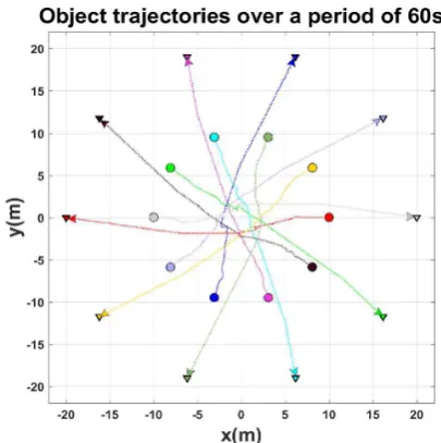
In this section we demonstrate the conflict resolution meth-ods outlined in Section III. The agent population is initialised with the parameters defined in Table I. The noise parameters are applied to better represent sensor-derived measurement of the obstacle trajectory. Agents are designated a target way-point at the antipodal position of a concentric circle with a radius of20m. The agents are tasked with crossing the circle to reach their way-point positions~pwp,iwhilst avoiding collision.

In Figure 6 the agent initialise at their origins (circles) and move through the collision centre to reach their respective way-points (triangles).

Events such as collisions or way-point incidence are said to occur when the following condition is violated||~pi−p~wp,i||<

(ri+rwp,i)−Ktol, where the parameterKtol is a condition

tolerance that aims to eliminate ambiguity between collisions and narrow-misses caused by the nature of discrete simulation.

Parameter Value

Maximum speed 2 m/s

Agent critical radius 0.5 m

Neighbour horizon 15 m

Camera standard deviation 5.208×10−5 rad Range-finder standard deviation 0.5 m Airspeed standard deviation 0.5 m/s Position standard deviation 0.5 m

Agent orbital radius 10 m

Way-point orbital radius 20 m

Object position standard deviation 0.5 m

Cycles 1000

Sampling rate 0.25 s

Event tolerance (Way-points, Collisions etc..) 1×10−3m

TABLE I

THE UNILATERAL AGENT PARAMETERS,INCLUDING ASSUMPTIONS ON

SENSOR UNCERTAINTY.

Fig. 6. A depiction of ten agents using theVObased reactive avoidance in a concentric collision scenario. The oscillations due to obstacle compensative motion can be clearly observed as the agent progress towards the collision centre.

The agent and scenario parameters are otherwise explicitly stated in Table I.

The selected algorithms presented in Section III were placed in scenarios with an increasing numbers of agents. We examine the ten agent scenario to discuss the principle difference in algorithm behaviour. Figure 6 demonstrates the trajectories generated by the VO algorithm. When compared to the RVO

in Figure 7 the trajectory adjustments can be seen to be abrupt, with greater oscillation throughout, until all conflicts are resolved.

The compensation for obstacle movement is clearly seen in Figure 7 as the trajectories are shown more gradual. This indicative of the adjustment of the RVO in response to the movement of the obstacles; leading to fewer instances of harsh correction. Oscillation in the form ofReciprocal Dancecan still be observed however as the direction of pass is resolved.

Fig. 7. A depiction of the ten agent concentric scenario and applying theRVO based avoidance method. Abrupt trajectory changes can be seen observed, with distinct oscillations as new agentsjenter the visual horizon of agenti.

Fig. 8. The ten agent concentric scenario repeated with theHRVOobstacle generation method applied. Oscillations can be observed as the procedure begins, however shown to be near linear as the direction of pass is resolved.

in Figure 8; their is a clear reduction in the oscillation as the agents initially determine their direction of pass. The

HRVO directional bias can also be observed from the agent trajectories, indicated by the emergent spiral behaviour around the conflict centre.

The representation of theVOasORCAconstraints is shown to produce trajectories similar to that the ofHRVOin Figure 9. The linearity of the of the constraints however is shown to create smooth trajectories throughout the conflict scenario, resulting in a smaller overall course deviations.

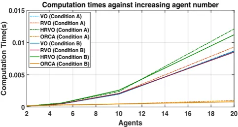
The selected algorithms were exampled in scenarios with 2, 5, 10 and 20 agents and their performance measured over 1000 Monte Carlo independent iterations. In addition to this, two sensor conditions were observed; A)Ideal Sensing; the agents

Fig. 9. The ten agent concentric scenario repeated under theORCAobstacle generation method. The resultant trajectories appear as smoother, more gradual adjustments than the previous methods.

are given perfect knowledge of the surrounding obstacles B)

Representative Sensing; the agents adopt the sensor properties defined in Table I.

Algorithm Condition

Mean Collisions

Mean Minimum Separation (m)

Mean Computation

Time (ms)

Condition A

VO 9.203 0.581 2.000

RVO 3.140 0.831 2.100

HRVO 0.053 0.996 2.400

ORCA 0.038 1.000 0.460

Condition B

VO 7.749 0.624 2.000

RVO 9.380 0.577 2.100

HRVO 2.878 0.836 2.600

ORCA 6.881 0.757 0.463

TABLE II

ALGORITHM PERFORMANCE OF IN THE SAME10AGENT SCENARIO. CONDITIONA) SENSING CAPABILITIES ARE ASSUMED IDEAL, CONDITION B) ASSUMING REPRESENTATIVE SENSING. EACH VALUE REPRESENTS THE

MEAN ACROSS1000INDEPENDENTMONTECARLO ITERATIONS.

2 4 6 8 10 12 14 16 18 20 Agents 0 0.005 0.01 0.015 Computation Time(s)

Computation times against increasing agent number

VO (Condition A) RVO (Condition A) HRVO (Condition A) ORCA (Condition A) VO (Condition B) RVO (Condition B) HRVO (Condition B) ORCA (Condition B)

Fig. 10. The mean algorithm computation times in both condition A) Ideal obstacle knowledge is assumed B) Obstacle telemetry data is subject to interference. Their effect on computation time is observed with an increasing number of obstacles.

Observing the behaviour of the algorithms in the presence of sensor uncertainty demonstrated a 5.08% mean increase in computation time. This can be seen more clearly in Figure 10. The RVO is shown to be sensitive to obstacle trajectory uncertainty; with a factor of 3 increase in mean collision likelihood across the 1000 iterations. This may be due the aggravation of the reciprocal corrections (Reciprocal Dance) by the uncertainty in obstacle trajectory. Similar behaviour can also be observed for the ORCA algorithm, as the sensor uncertainty is shown to significantly increase the likelihood of collision under this regime also.

The ORCA algorithm was also shown to have achieved a mean minimum separation closest to the desired 1m. This suggests theORCAalgorithm was more consistent in its ability to maintain the intended boundary condition. Although, in considering noisy telemetry this resulted in a mean collision likelihood 40.03% higher than theHRVO approach.

Studying Figure 10, we observe an exponential relationship between the size of the agent population and the mean algo-rithm computation time for theVO,RVOandHRVOmethods. TheORCAapproach is however shown to benefit greatly from the linear representation of the constraint set; computation time is shown to scale linearly with increasing agent number. The relationship between the performance reduction raterORCA=

3.4×10−5_s/n

is shown to be distinctly lower than the other presented approaches. The ORCA algorithm therefore has a clear advantage when considering scalability for larger multi-agent systems, abeit more susceptible to uncertainty than the

HRVO method. All analyses were completed using an Intel Core i7-6600HQ quadcore (@2.8GHz) CPU. Code for the presented algorithms and scenarios are also available on Github [18].

VI. CONCLUSIONS

In this paper several well established approaches to non-cooperative collision avoidance are presented for use in multi-agent systems. Uncertainty in obstacle trajectory is shown to increase the mean computation time of all the proposed approaches by without compensative measures. The HRVO

and ORCA methods are shown to be more effective in both

negotiating dense environments without collision, and handing obstacle trajectory uncertainty. The ORCA method is also shown to generate both smoother resolution trajectories and scalable mean computation times.

The presented algorithms have shown that reactive collision avoidance can be sufficient to mitigate multiple collisions in a communication denied environment. Further work into inherent avoidance will examine such algorithms in the presence static and dynamic obstacles in more sophisticated coordinated tasks.

REFERENCES

[1] A. Zhahir, A. Razali, and M. Ajir, “Current Development of UAV Sense and Avoid System,” inProc. of the IOP Conference on Materials Science and Engineering, vol. 152, Universiti Putra Malaysia, 2016.

[2] S. Ramasamy and R. Sabatini, “A Unified Approach to Cooperative and Non-Cooperative Sense-and-Avoid,” in Proc. of the International Conference on Unmanned Aircraft Systems, ICUAS 2015. IEEE, 2015, pp. 765–773.

[3] J. Douthwaite, A. D. Freitas, and L. Mihaylova, “An interval approach to multiple unmanned aerial vehicle collision avoidance,” in Proc. of the 11th Symposium Sensor Data Fusion: Trends, Solutions, and Applications, SDF 2017. IEEE, September 2017.

[4] J. Marin, R. Radtke, D. Innis, D. Barr, and A. Schultz, “Using a genetic algorithm to develop rules to guide unmanned aerial vehicles,” inProc. of the IEEE International Conference on Systems, Man, and Cybernetics (SMC), vol. 1, 1999, pp. 1055–1060.

[5] A. Richards and J. How, “Aircraft Trajectory Planning with Collision Avoidance using Mixed Integer Linear Programming,” inProc. of the American Control Conference, vol. 3, no. 2, 2002, pp. 1936–1941. [6] H. Chen, V. Jilkov, and X. Li, “On threshold optimization for aircraft

conflict detection,” inProc. of the 18th International Conference on Information Fusion, Fusion 2018. IEEE, 2015, pp. 1198–1204. [7] M. Suzuki and K. Uchiyama, “Three-Dimensional Formation Flying

Using Bifurcating Potential Fields,” in Proc. of the AIAA Guidance, Navigation and Control, vol. 22, 2009, pp. 1753–1759.

[8] P. Fiorini and Z. Shiller, “Motion Planning in Dynamic Environments Us-ing Velocity Obstacles,”The International Journal of Robotics Research, vol. 17, no. 7, pp. 760–772, 1998.

[9] D. Wilkie, J. van den Berg, and D. Manocha, “Generalized Velocity Obstacles,” inProc. of the International Conference on Intelligent Robots and Systems. IEEE, 2009, pp. 5573–5578.

[10] J. van den Berg, M. Lin, and D. Manocha, “Reciprocal Velocity Obstacles for Real-Time Multi-Agent Navigation,” inProc. of the International Conference on Robotics and Automation. IEEE, 2008, pp. 1928–1935. [11] V. G. Santos, M. F. Campos, and L. Chaimowicz, “On segregative behav-iors using flocking and velocity obstacles,” inDistributed Autonomous Robotic Systems. Springer, 2014, pp. 121–133.

[12] J. van den Berg, J. Snape, S. Guy, and D. Manocha, “Reciprocal Collision Avoidance with Acceleration-Velocity Obstacles,” inProc. of the International Conference on Robotics and Automation, 2011, pp. 3475–3482.

[13] J. Snape, J. van den Berg, S. J. Guy, and D. Manocha, “The Hybrid Reciprocal Velocity Obstacle,”IEEE Transactions on Robotics, vol. 27, no. 4, pp. 696–706, 2011.

[14] M. Kim and J. Oh, “Study on Optimal Velocity Selection using Velocity Obstacle (OVVO) in Dynamic and Crowded Environment,”Autonomous Robots, vol. 40, no. 8, pp. 1459–1470, 2016.

[15] Z. Shiller, F. Large, S. Sekhavat, and C. Laugier, “Motion Planning in Dy-namic Environments: Obstacles Moving Along Arbitrary Trajectories,” inProc. of the International Conference on Robotics and Automation, vol. 4, Grenoble, France, 2001, pp. 3716–3721.

[16] J. Wilkerson, J. Bobinchak, M. Culp, J. Clark, T. Halpin-Cha, K. Es-tabridis, and G. Hewer, “Two-Dimensional Distributed Velocity Collision Avoidance,” Naval Air Warfare Center Weapons Division, Tech. Rep. February, 2014.

[17] J. Van Den Berg, S. Guy, M. Lin, and D. Manocha, “Reciprocal n-body collision avoidance,” inRobotics research. Springer Tracts in Advanced Robotics, 2011, vol. 70, pp. 3–19.