This is a repository copy of Development of Constrained Predictive Functional Control
using Laguerre Function Based Prediction.
White Rose Research Online URL for this paper:
http://eprints.whiterose.ac.uk/113412/
Version: Accepted Version
Proceedings Paper:
Abdullah, M., Rossiter, J.A. orcid.org/0000-0002-1336-0633 and Haber, R. (2017)
Development of Constrained Predictive Functional Control using Laguerre Function Based
Prediction. In: IFAC-PapersOnLine. 20th IFAC World Congress, 09/07/2017 - 14/07/2017,
Toulouse, France. Elsevier , pp. 10705-10710.
https://doi.org/10.1016/j.ifacol.2017.08.2222
Article available under the terms of the CC-BY-NC-ND licence
(https://creativecommons.org/licenses/by-nc-nd/4.0/)
[email protected] https://eprints.whiterose.ac.uk/
Reuse
This article is distributed under the terms of the Creative Commons Attribution-NonCommercial-NoDerivs (CC BY-NC-ND) licence. This licence only allows you to download this work and share it with others as long as you credit the authors, but you can’t change the article in any way or use it commercially. More
information and the full terms of the licence here: https://creativecommons.org/licenses/
Takedown
If you consider content in White Rose Research Online to be in breach of UK law, please notify us by
Development of Constrained Predictive
Functional Control using Laguerre Function
Based Prediction
M. Abdullah∗,∗∗ J.A. Rossiter∗ R. Haber∗∗∗
∗Department of Automatic Control and System Engineering,
University of Sheffield, Mappin Street, S1 3JD, UK. (e-mail: [email protected], [email protected])
∗∗Dept. of Mech. Engin., International Islamic University Malaysia.⋆ ∗∗∗Institute of Process Engineering and Plant Design, Cologne
University of Applied Sciences, D-50679 K¨oln, Germany.
Abstract: This work presents a novel constraint handling strategy for Predictive Functional
Control (PFC). First, to improve prediction consistency, the constant input assumption of nominal PFC approaches is replaced with Laguerre based prediction. This substitution improves the effectiveness of using a constrained solution to prevent long-term constraint violations. Secondly, for state constraints, a simpler single regulator approach is proposed instead of switching between regulators, an approach common in the PFC literature. Simulation results verify that the proposed method manages the constraints better than the traditional approach. Moreover, despite all the modifications, the controller formulation and framework remain simple and straightforward which thus are in line with the key ethos of PFC.
Keywords:Predictive Control, Constrained PFC, Effective Constraint Technique.
1. INTRODUCTION
Most control systems have constraints which can be identi-fied as input constraints, rate constraints, state constraints and output constraints. If these constraints are not consid-ered systematically in a control design, it may result in un-wanted behaviour such as overshoots, long settling times, and even instability. Satisfying constraints effectively offers many attractive benefits including a higher production profit, better control performance, lower maintenance cost and safer control environment (Rossiter, 2003; Richalet and O’Donovan, 2009; Wang, 2009; Abdullah and Idres, 2014a). Clearly, these scenarios justify the need for a systematic constrained controller design.
In practice, the commonly used Proportional-Integral-Derivative (PID) controller faces difficulties in handling constraints. For example, the usage of an integrator during constraint violations can produce wind-up and/or satura-tion (Rossiter, 2003). Although, anti wind-up techniques can prevent this situation (Visioli, 2006), these require tuning procedures which are difficult to design and manage for different combinations of dynamics and constraints.
Conversely, Model Predictive Control (MPC) utilises a representative mathematical model to form an accurate future prediction of the system behaviour and thus sat-isfies constraints systematically via an optimal control approach (Rossiter, 2003; Wang, 2009). However, typical MPC strategies require a high computational demand and expensive computer hardware, thus are only suitable for
⋆ This work is funded by International Islamic University Malaysia
and Ministry of Higher Education Malaysia.
certain applications (Rossiter et al., 2010; Jones and Kerri-gan, 2015). Indeed, as the number of constraints increases, the optimal constraint handling problem requires increas-ingly complex and demanding solvers.
Many industrial end-users are willing to trade off some loss in optimality with ease/cost of implementation. This preference has triggered the widespread acceptance of Pre-dictive Functional Control (PFC) among industrial prac-titioners. PFC belongs to the family of predictive control which compute the manipulated input based on a sim-plified cost function. It provides some valuable properties namely intuitive tuning, simplicity in coding, low com-putational demand, effective handling of dead-time pro-cesses and a basic constraint handling ability (Richalet and O’Donovan, 2009). With these features, PFC has become a popular and widely used alternative to PID controllers, especially for SISO loops.
constraints, where multiple regulators that work in parallel are switched either to track the set point or satisfy the constraint depending on a supervisor decision (Richalet and O’Donovan, 2009). This structure works in most appli-cations, but has a disadvantage in that it requires a careful tuning procedure to avoid conflicts with the internal con-straints which thus counters some of the inherent benefits of a simple and transparent approach. The operation cost also may increase due to the use of multiple regulators.
This paper proposes a better constraint strategy to allevi-ate some of the drawbacks of the conventional approach. A Laguerre function will be utilised to improve the pre-diction consistency (Abdullah and Rossiter, 2016), hence instead of assuming a constant future value, the future predicted input converges to the steady state exponentially based on the desired pole. With a well-posed decision, the constrained solution will become more precise and less conservative. In addition, rather than handling state constraints with a multiple regulators scheme, a vector approach is considered to simplify the computation and tuning processes.
Section 2 provides a brief description of a traditional con-strained PFC formulation. Section 3 presents the proposed Laguerre PFC scheme for constraint management. Section 4 gives a comparison between the nominal and Laguerre approaches based on two numerical examples. Finally, section 5 presents some conclusions and future work.
2. NOMINAL CONSTRAINED PFC FORMULATION
This section provides a brief review of nominal PFC in-cluding constraint handling. For simplicity of presentation of the core concepts, the main objective is to track a con-stant step target and moreover, the offset correction and integral action algebras are omitted, although included in the numerical examples. These simplifications do not affect the core analysis, insights and results presented. Finally, without loss of generality, the PFC formulation is constructed using a general transfer function structure.
2.1 Unconstrained PFC
The basic principle of PFC is to drive the ny step ahead prediction of output yk+ny|k nearer to the set point R than the current outputyk. The ratio is linked to a tuning parameter is the desired closed loop poleλ=e−3T /CLT R, where T is the sampling time and CLTR is the desired closed loop settling time (to 95%). The basic PFC law is defined by enforcing the following equality:
yk+ny|k =R−(R−yk)λ
ny (1) whereny is denoted as the coincidence horizon. There are some subtleties to ensure offset free tracking but the basic law is still (1). For a more detailed description of PFC theory and concepts, interested readers can refer to these references, e.g. (Rossiter and Haber, 2015; Richalet and O’Donovan, 2009; Haber et al., 2011).
Since the prediction algebra for general transfer functions is well known in the literature (e.g. (Rossiter, 2003)), only simplified formulations are presented here. The ny step ahead unbiased linear prediction for inputsukand outputs
yk can be represented as:
yk+ny|k=Hnyu→k+Pnyu←k+Qnyy←k (2)
whereHny,Pny,Qny depend on the model parameters and for systems of orderm:
uk
→ =
uk
uk+1
.. .
uk+n−1
;u←k =
uk−1
uk−2
.. .
uk−m
;y←k=
yk
yk−1
.. .
yk−m
(3)
The control input is solved by substituting the predic-tion of (2) into (1) alongside the assumppredic-tion of a con-stant future input, namely uk+i|k = uk, i = 0, ..., ny. In consequence the parameter Hny can be simplified to
hny =Hny[1,1,· · ·]
T and (1) becomes:
hnyuk+Pnyu←k+Qnyy←k=R−(R−yk)λ
ny (4) After minor rearrangement, the, PFC law reduces to:
uk=
R−(R−yk)λny −(P
nyu←k+Qnyy←k)
hny
(5)
2.2 Input and Input Rate Constraints
The system input is often constrained because of physical limits or indeed desired limits on temperature, pressure, voltage and others. These constraints are presented as:
umin≤uk≤umax (6) ∆umin+uk−1≤uk≤∆umax+uk−1 (7)
where ∆umin and ∆umax are the minimum and the maximum rate, whileumin andumaxdenote the minimum and maximum input. Without explicitly including these constraints in the control computation, a clipping method can be utilised (Fiani et al., 1991). When the limit in (6) or (7) is violated, the controller will treat it as an equality constraint (Wang, 2009). However, it is crucial for the model to detect possible constraint violationsa priori
(Richalet and O’Donovan, 2009). Failure to do this could introduce an overshoot in the input (and/or output) due to a mismatch between the predicted model behaviour and the actual system behaviour.
Remark 1. The input and rate constraint need only be implemented on the current input within conventional PFC because of the constant future input assumption.
2.3 State Constraints
In some applications (i.e heat treatment) an internal variable, state or output may be constrained either for an economic or safety reason. To solve this problem, the conventional PFC approach uses multiple regulators which run in parallel (see Fig. 1) (Richalet and O’Donovan, 2009; Fiani et al., 1991).
• The first regulatorP F C1is the preferred control law
and produces input u1,k (using (5)) to track the set point while satisfying its internal constraints. Within some validation horizon to be defined, the supervisor uses input u1,k to predict the future state behaviour using a prediction model such as (2). If the state predictions are within their limit, then useuk =u1,k.
• The second regulator P F C2 is more conservatively
tuned and tracks the state limit by manipulating input u2,k. When the state limit is expected to be
Fig. 1. Schematic of PFC considering state constraints.
• An advanced decision-making method such as fuzzy logic, look up table, or artificial neural network may be utilised for a smoother transition.
Remark 2. The second controllerP F C2 regulates the
sec-ond inputu2,k based on a state prediction equation:
xk+nx|k =hnxuk+Pnxu←k+Qnxx←k (8) where hnx, Pnx, Qnx denote the state model parameters. The maximum state limit xmax is a set as a target. With a suitable coincidence horizon nx and the desired closed loop poleλx, inputu2,k is computed as:
u2,k =
xmax−(xmax−xk)λnx
x −(Pnxu←k+Qnxx←k)
hnx
(9)
The associated PFC is tuned, if possible, to avoid oscilla-tions in the predicoscilla-tions to ensure the constraint is satisfied.
Remark 3. A suitable validation horizon for checking the predictions associated to P F C1 should be used since the
projection ofu1,k
→ must include the open loop time response
ofP F C2. In addition, the target poleλxofP F C2must be
compatible with the need to satisfy the internal constraints of P F C1. Choosing a fast pole to improve the overall
system response may decrease the controller robustness and introduce conflicts with the actuator limit (Richalet and O’Donovan, 2009).
3. CONSTRAINED LAGUERRE PFC FORMULATION
This section presents the formulation of PFC based on Laguerre based input predictions. By embedding expo-nentially decaying dynamics within the input prediction, it enables PFC to achieve a closer match to the desired closed-loop behaviour. This can improve the reliability of the constrained PFC solution. A detailed analysis and benefits of Laguerre PFC are presented in Abdullah and Rossiter (2016). Since a similar strategy to nominal PFC is adopted for input and rate constraints (Remark 1), only the state/output constraint case is presented here.
The Laguerre PFC approach requires explicit knowledge of the expected constant steady-state input uss which will lead to no steady-state offset; in fact this value is implicitly used in conventional MPC as well. For a given model and disturbance estimate, the computation of this is straightforward (Rossiter, 2003).
3.1 Unconstrained Laguerre PFC formulation
A Laguerre polynomial is often used for system identifica-tion and estimaidentifica-tion as it can provide the ability to capture system behaviour with fewer parameters (Nurges, 1987). The z-transform of discrete Laguerre polynomials are:
Lj(z) =
p
1−a2(z
−1−a)j−1
(1−az−1)j ; 0< a <1 (10)
where j is the order of Laguerre function and a is the Laguerre pole which depends on a user selection. Although a high order polynomial can be used in MPC (Abdullah and Idres, 2014b; Wang, 2009), this work employs a first-order Laguerre polynomial to retain the simplicity of formulation especially when dealing with low order system. The first-order Laguerre function, with altered scaling is:
L1(z) =
1
1−az−1 ≡ 1 +az
−1+a2z−2+· · · (11)
DefineL1= [1, a, a2,· · ·, an−1]T. Now we are in a position
to define the input prediction to be deployed in PFC.
Theorem 1. A future input parametrised as
u(z) = uss 1−z−1 +
η
1−az−1 (12)
will give output predictions which settle at the desired steady-state.ηrepresents one degree of freedom.
Proof:The signal defined in (12) has the property that
lim
k→∞uk =uss ⇒ klim→∞yk=R (13)
The implied input prediction in (12) converges to the steady state exponentially with a rate a. The associated output prediction is derived by substituting (12) into (2):
yk+ny|k =hnyuss+HnyL1η+Pnyu←k+Qnyy←k (14)
The following algorithm defines the PFC law using the Laguerre polynomial to shape the input predictions.
Algorithm 1.(LPFC). Define theny step ahead predicted output using equation (14). The PFC law is defined by substituting this prediction into (1), solving for the parameterη and then computinguk from (12).
η=R−(R−yk)λ ny −(P
nyu←k+Qnyy←k)−hnyuss
HnyL1
(15)
Due to the receding horizon principle (Wang, 2009) and the definition ofL1(z), the current input is defined as:
uk =uss+η (16)
Remark 4. The value of Laguerre pole a determines the convergence speed of a system (Abdullah and Rossiter, 2016). For low order system, a reasonable choice isa=λ
where it gives a direct link to the desired target trajectory.
Remark 5. The maximum (if bigger than uss) and mini-mum (if smaller than uss) of the predicted future input given in (12) is the first (current) value uk. Similarly, the maximum/minimum rate is given from ∆uk =uss+
η −uk−1. Hence, with LPFC, the maximum/minimum
input rate/value (relative to expected steady-state) occur at the first sample and thus the proposed Laguerre PFC can adopt an equivalent constraint handling procedure for input constraints as standard PFC.
3.2 Efficient state and output constraint handling
Lemma 2. The input constraints can be represented by a set of linear inequalities with a single variableη.
Proof: This follows directly from the observations in
remark 5. The constraints can be summarised as follows:
1 −1 1 −1
η+
uss
−uss
uss−uk−1
uk−1−uss
≤ umax umin ∆umax ∆umin
(17)
Lemma 3. State constraints can be represented by a set of linear inequalites with a single variableη.
Proof:This follows directly from computation of the state
predictions as in (14) and comparison with the state limits. For example, a single state limit gives the following:
Hnx
uss uss uss .. . + 1 a a2 .. . η
+Pnxu←k+Qnxx←k
| {z }
fnx(k)
≤xmax
One can stack these inequalities over a specified horizon such that, for example:
H1 H2 . . . uss uss . . . + 1 a . . . η + f1(k)
f2(k)
. . .
≤xmax (18)
Theorem 4. All the input, state and output constraints can be represented by a single vector inequality as:
M η≤v(k) (19)
Proof:This is a consequence of the previous two lemmata
by combining all the inequalities for all the constraints. The vector M is fixed but the vector v(k) varies each sample as it depends upon past system data and the estimation of the expected steady-state inputuss.
Corollary 1. In the absence of uncertainty, the inequalities implied in (19) are always feasible, assuming feasibility at the previous sample, no changes in the target and a long enough horizon.
Proof:The structure of the input prediction (12) is such
that, as long as uss does not change from one sample to the next, then one can always choose η so that the predicted input trajectory is unchanged; this is obvious from the simple exponential structure. Consequently, if there exists an η to satisfy constraints at the previous sample, there must exist a valid value at the current sample. [We shall not discuss issues linked to required horizon lengths (Gilbert and Tan, 1991) as this would take the complexity beyond reasonable expectations for PFC approaches where a lack of rigorous mathematical guarantees is accepted to allow more simplicity.]
Remark 6. Infeasibility can arise due to too fast or too large changes in the target (or disturbances) as this causes large changes in the value ofuss. However, Laguerre PFC helps enormously in this case because the exponential structure embedded into the input prediction automati-cally slows down any over aggressive input responses and thus significantly increases the likelihood of feasibility be-ing retained. In the worst case, set point changes need to be moderated (as in reference governer approaches) but such a discussion is beyond the remit of this paper.
We can now define the constraint handling algorithm.
Algorithm 2.(LPFC constrained). First ensure that the change in the steady-state value of uss is such that no absolute or rate constraints in the inputs are violated as this suggests a poorly chosen target. Hence enforce that
|uss,k−uss,k−1|<∆umax and thatumin≤uss≤umax. Second, use the unconstrained law (15) to determine the ideal value ofη and check each constraint implied in (19) using the following simple loop (subscripts denote position in a vector).
Setηmax=∞, ηmin =−∞. For i=1:end,
ifMiη6≤vi &Mi>0 then defineηmax=vi/Mi, ifMiη6≤vi &Mi<0 then defineηmin=vi/Mi, end loop.
ifη < ηmin, setη=ηmin. ifηmax< η, set η=ηmax. Note that the upper and lower limits on η to ensure feasibility update at each cycle in the loop but as all the inequalities are only ever tightened, changes lower down cannot contradict changes higher up.
3.3 Summary of benefits
This approach eliminates the careful tuning process of multiple regulators (Remark 3) since the constraint is now explicitly included in the control computation. Moreover, the algebra for computing the vectors v, M is the same as that required for computing the predictions and thus is unavoidable where constraint handling is desired and specifically, needs no input or tuning choices from the designer. This work has not investigated the implications of infeasibility due to large disturbances or set point changes any further than insisting on sensible limits to changes in uss as that is a more challenging scenario and requires a priori trade off decisions such as which constraints or requirements to sacrifice during transients.
4. NUMERICAL EXAMPLES
This section presents two numerical examples to highlight the benefit of the proposed constraint method. The first example implements output constraints while the second example operates with state constraints. For each case, two figures are plotted to represent the system input and output. The focus is to analyse and compare the constrained control performance of nominal PFC (PFC) and Laguerre PFC (LPFC). It should be noted that throughout the examples, a choice of a = λ is used for LPFC as discussed in Remark 4.
4.1 Output Constraint Example
A first order system (20) with 0.2 input disturbance from 20sto 25sshould track a constant set point (R= 1). For a fair comparison of PFC and LPFC, both controllers use similar tuning parameters for the desired pole (λ = 0.7) and a coincidence horizon (ny= 1).
G1= 0.25z −1
1−0.8z−1 (20)
Samples
0 5 10 15 20 25 30 35 40
Intput
0 0.2 0.4 0.6 0.8 1 1.2 1.4 1.6
u (PFC) u
p (PFC)
u (LPFC) u
p (LPFC)
Samples
0 5 10 15 20 25 30 35 40
Output
0 0.2 0.4 0.6 0.8 1 1.2 1.4 1.6
y (PFC) y
p (PFC)
y (LPFC) y
p (LPFC)
[image:6.595.346.510.75.354.2]r
Fig. 2. Unconstrained PFC and LPFC responses.
trajectoryR with settling time 8 samples and overshoots slightly in response to the disturbance. However, the initial prediction of nominal PFC yp(P F C) (displayed as com-puted at the first sample) is inconsistent with the actual closed-loop behavioury(P F C) because of the assumption of constant input in the prediction (i.e.up(P F C)). Never-theless, the actual inputu(P F C) converges to the correct steady state value. Since LPFC embeds the exponential decay dynamics (e.g. through (12)), the input prediction
up(LP F C) matches the actual system input u(LP F C) and so has better consistency between predictions and ac-tual behaviour. This consistency is important for accurate constraint handling, to avoid conservativeness.
For the constrained case, a maximum output is set at
ymax = 1.05. A validation horizon i = 10 is used to cover the transient period and avoid a long-term violation. However, PFC detects the output violation ofyp(P F C) at the 6th sample ahead because of the ill-posed prediction (refer Fig. 2). The constraint is satisfied (Fig. 3) by the input u(P F C) reducing from 1.2 to 0.9. As a result, the output y(P F C) converges slower to the set point compared to y(LP F C). Since LPFC produces a well-posed prediction, the output y(LP F C) exactly matches the target trajectoryR with a precise solutionu(LP F C).
4.2 State Constraint Example
Consider two processes that run in parallel. The main processP1and state processP2receive a similar
manipu-lated inputufrom the regulator. For safety and economic reasons, the state is constrained at xmax = 127 with a limited input umax= 160, and speed ∆umax= 4.
P1= 0.0164z−
1
1−0.9835z−1;
P2= 0.08914z−
1−0.08674z−2
1−1.918z−1+ 0.92z−2 (21)
Samples
0 5 10 15 20 25 30 35 40
Intput
0 0.2 0.4 0.6 0.8 1 1.2
u (PFC) u (LPFC)
Samples
0 10 20 30 40 50
Output
0 0.2 0.4 0.6 0.8 1 1.2
y (PFC) y (LPFC) r y
[image:6.595.81.246.75.356.2]max= 1.05
Fig. 3. Constrained PFC and LPFC responses.
For a fair comparison, Laguerre PFC (LPFC) and the first regulator of state constrained PFC (CPFC) will both use
ny = 1, validation horizon (i = 68) and pole (λ= 0.975) to track the set point (R = 100). Since CPFC treats the maximum state as a second target (9), the coincidence horizon (nx = 30) and desired pole (λx = 0.984) of the second constraining regulator are selected carefully to satisfy the internal constraints (Remark 3).
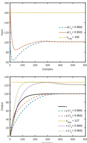
Fig. 4 shows that LPFC outperforms CPFC while satisfy-ing the state constraints. Although the state behaviours of both x(CP F C) andx(LP F C) are within the limits, the output settling time of y(LP F C) 200 samples is almost twice as fast as y(CP F C) (300+ samples) and closer to the target trajectory R. In addition, CPFC requires a careful tuning process and a higher operation cost as two regulators are used simultaneously. To respect the actuator limits, a large pole is needed to slow down the control response. Fig. 5 demonstrates the effect of poor tuning decision with a smaller pole λx = 0.963, where it computes a higher initial input than the maximum input xmax = 160. On the other hand, LPFC satisfies all the system constraints systematically without conflict. With Laguerre based prediction, the constrained solution becomes more precise and less conservative compared to the nominal CPFC approach.
5. CONCLUSION
Samples
0 100 200 300 400 500 600
Input
40 50 60 70 80 90 100 110
u
2 (CPFC) active u1 (CPFC) active
u (CPFC) u (LPFC)
Samples
0 100 200 300 400 500 600
Output
0 20 40 60 80 100 120 140
r y (CPFC) y (LPFC) x
max = 127
[image:7.595.79.247.76.355.2]x (CPFC) x (LPFC)
Fig. 4. Constrained CPFC and LPFC reponses.
Samples
0 100 200 300 400 500 600
Input
60 80 100 120 140 160 180
u(λ x= 0.984)
u(λ x= 0.963)
u
max= 160
Samples
0 100 200 300 400 500 600
Output
0 20 40 60 80 100 120 140
r y (λ
x= 0.984)
y (λ x= 0.963)
x
max = 127
x (λ x= 0.984)
x (λ x= 0.963)
Fig. 5. CPFC responses with different poles λx = 0.984 andλx= 0.963.
input dynamics instead of constant input dynamics gives a better prediction consistency which ensures the constraint handling is more precise and less conservative. Given that the more conservative and complicated multi-regulator ap-proach is widely adopted in many industrial applications,
we expect the proposed single constrained LPFC will offer better performance and be more cost effective. It alleviates the strict tuning requirements of the second CPFC regu-lator while satisfying all the constraints in a systematic fashion. As shown in the examples, the proposed method often enables faster convergence when handling the output and state constraints compared to the nominal strategy.
For future work, the robustness and sensitivity analysis of conventional PFC and LPFC will be investigated as well as the potential for more rigorous stability and feasibility guarantees, while retaining simplicity. Moreover, tests on hardware are planned. Finally, consideration will focus on whether higher order input parameterisations would be even more advantageous for higher order systems; this may involve a more complex constraint handling procedures.
REFERENCES
Abdullah, M. and Idres, M. (2014a). Constrained model predictive control of proton exchange membrane fuel cell. JMST, 28(9), 3855–3862.
Abdullah, M. and Idres, M. (2014b). Fuel cell starvation control using model predictive technique with Laguerre and exponential weight functions. JMST, 28(5), 1995– 2002.
Abdullah, M. and Rossiter, J.A. (2016). Utilising Laguerre function in predictive functional control to ensure pre-diction consistency. UKACC.
Fiani, P., Richalet, J., et al. (1991). Handling input and state constraints in predictive functional control. In
CDC, 985–990. IEEE.
Gilbert, E.G. and Tan, K.T. (1991). Linear systems with state and control constraints: The theory and application of maximal output admissible sets. IEEE Transactions on Automatic Control, 36(9), 1008–1020. Haber, R., Bars, R., and Schmitz, U. (2011). Predictive
control in process engineering:From basics to applica-tions, chapter 11. Wiley-VCH, Germany.
Jones, C.N. and Kerrigan, E. (2015). Predictive control for embedded systems. Optimal Control Applications and Methods, 36(5), 583–584.
Nurges, Y. (1987). Laguerre models in approximation and identification of digital systems. Avtomatika i Telemekhanika, (3), 88–96.
Richalet, J. and O’Donovan, D. (2009). Predictive func-tional control: principles and industrial applications. Springer.
Rossiter, J.A. (2003). Model-based predictive control: a practical approach. CRC press.
Rossiter, J., Kouvaritakis, B., and Cannon, M. (2001). Computationally efficient algorithms for constraint han-dling with guaranteed stability and near optimality.IJC, 74(17), 1678–1689.
Rossiter, J., Wang, L., and Valencia-Palomo, G. (2010). Efficient algorithms for trading off feasibility and per-formance in predictive control. IJC, 83(4), 789–797. Rossiter, J.A. and Haber, R. (2015). The effect of
coin-cidence horizon on predictive functional control. Pro-cesses, 3(1), 25–45.
Visioli, A. (2006). Practical PID control. Springer. Wang, L. (2009). Model predictive control system design
[image:7.595.77.246.394.670.2]