Pixel Based Sar Image Classification using Random Forest Algorithm

(1)

International Journal of Innovative Technology and Exploring Engineering (IJITEE) ISSN: 2278-3075,Volume-8 Issue-10, August 2019



Abstract: Synthetic Aperture Radar (SAR) images (Microwave data) were classified using Multi-Layer Feed Forward, Cascade Forward Neural Networks and Random Forest (RF) algorithms.

For the Random Forest, a general model for classification of Remotely Sensed Radar dual-polarization data based on RF is implemented and classified of SAR image (microwave data) classifications. The RF model exploits spatial context between neighbouring pixels in an image, and temporal class dependencies between different images of the same region, in the case of multi-temporal data. Based on the well-founded experimental on basis of random forest techniques for classification tasks and the encouraging experimental results in RF algorithm , the authors conclude that the proposed RF algorithm is useful for classification of SAR (Sentinel 1A) imagery and evaluate its accuracy and kappa coefficient.

Keywords: Cascade feed forward neural network, Multilayer Feed forward, Random Forest, Synthetic Aperture Radar (SAR) Image Classifications.

I. INTRODUCTION

synthetic Aperture Radar (SAR) images are more difficult to understand, because of complicated interaction of microwaves with the Earth surface objects and speckle noise. They require careful analysis [1-2]. The main aim of the analysis is to streamline the description of the image data into quantifiable information which is realistic, highly understandable and accessible to use it as an input for applications. For example, the information of classification all pixels in the SAR images (microwave images) will be very much useful for planning and proper utilization of land. The procedure of segregating a digital image data, which consists of discrete forms or character, into various thematic partitions is known as pattern classification analysis. To state in another way, image analysis is a way of identification of each pixel in an image to a class, such that all pixels with similar identity or common qualities [3] belong to same class.

The major issue occurs during the analysis is clustering in the concentrated area [4]. Clustering is a famous autonomous motif analysis method which divides the group of n substances into k (>1) sets depending upon coincidences and non-coincidence metric where the value of k can either be pre-determined or not [5]. This paper explains the analysis and categorization utensil of the SAR image.

Revised Manuscript Received on August 12, 2019.

Battula Balnarsaiah, Research and Training Unit for Navigational Electronics (NERTU), Dept of ECE and University College of Engineering, Osmania University, Hyderabad, Telangana, India.

T.S.Prasad, National Remote Sensing Centre(NRSC), Indian Space Research Organization (ISRO), Hyderabad, Telangana, India.

P.Laxminarayana, Research and Training Unit for Navigational Electronics(NERTU), Osmania University, Hyderabad, Telangana, India.

A. Satellite image Analysis and Categorization The analysis of a satellite image into various synthesized regions, called ‘classes’ is one of the complicated issues [6] in the science of Image Analysis. The supervisory categorization methods are highly efficient. But, these methods need the appropriate guidance set, for every pixel of the new image to be classified. Generally, an individual does not have an idea about the various issues that exist in a SAR images. For example, the variation properties of the textures are not known clearly to locate where the textures are present. Similarly, in real-time or other applications, the possibility of deciphering relevant land use/cover information will not be present directly in many images. The major purpose of this paper is to examine some thriving categorization techniques of the day that provide accuracy for analyzing the images of the examined location where sufficient training information is facilitated. These techniques will help us in the effective usage of remote-sensing images [7].

The latest issue faced by the experimenters is by introducing an automatic conditioning method for maximum-likelihood (ML) segregation [8], which can develop a land-cover image even for the images for which perfect information is absent. Though Gaussian ML is operationally useful in Remote Sensing, search, modern methods can be utilized in future. Some of the modern algorithms which are believed to give better results are Neural Networks, Support Vector Machines, and Random Forest.

B. Supervised categorization technique This categorization technique is defined as below

Any pixel or dimensionally assembled sets of pixels revealing some factor, class, or object is distinguished by a level of digital numbers, for each of the bands of a remote sensor. The values of the digital numbers that are used for samples are taken as accumulated sets of information in 2D space for the thematic category. These are examined and determined analytically for finding their level of uniqueness in this spectral return space and some functional calculations are selected for segregating the clusters. The procedure commonly used in segregation is given below:

Supervised Classification

In the supervised categorization, the experimenter has an idea about the presence and location of the classes to enable provision of training samples. The person also should have (or desirable to have) an idea about, in how many locations the same class is present.

Pixel Based Sar Image Classification using

Random Forest Algorithm

(2)

These are placed on the image and the mathematical investigation is done on the multiband information present in every such class. The class groupings are also present in place of the cluster, and these groupings have suitable segregated operations. All pixels of the test images or sites for which class is not known, are correlated with the pixels of features of the known classes or sites, and the class is selected which is ‘nearer’ to the test pixel. In this paper, the classification results obtained by random forest method are compared with the results obtained by Multilayer Feed Forward Neural Networks (MFFNN) and Cascade Feed forward Neural Networks (CFFNN).

Supervised Classification

Fig.1.Supervised Categorization Principle Now the details of implementation of these three algorithms for classification of images are explained in Section-II, and the results and discussions in section III. Conclusion and future scope are given in section IV.

II.

I

MPLEMENTATION

A

LGORITHM

The principal algorithms in this work are Neural Networks and Random Forest. Neural Networks are inspired from biological phenomena [1]. For example, human beings are good at easy recognition of faces, handwritings, natural features like hills though for humans numerical processing is a bottleneck. In fact, human beings don’t perform any ‘visible’ complicated calculations for routine tasks such as recognition of known objects or persons. Computers, though highly suitable for numerical processing, aren’t that much good in identification of sometimes even simple objects.

A. Multi-Layer Feed-forward Neural Network

(MLFFNN)

In this work, the algorithm applied for multilayer feed-forward neural networks [9-10] is the back-propagation learning algorithm [11]. These neurons in this network are sequenced into layers, since human brain is assumed to have strata-like pattern. The initial layer is represented as the input layer and the final layer is represented as the output layer. The layers present in between the input and output layers are named as hidden layers, also sometimes called internal layers. To induce more nonlinear capabilities to the artificial neurons in the network, the neurons, upon will compute the weighted sum (integration) of receiving inputs from a previous layer, and transforms the computed integrated amount by using a non-linear function F, often called an activation function. Every neuron is a subset of ancestors or associates relatives of the represented neuron F . Every neuron present in the appropriate layer is linked with the neurons located in the upcoming layer. The links between

them and neurons of k and k-1 layers is weight coefficient and the threshold coefficient value given for the _{neuron is}_

i. The output value of the neuron is represented with , and its value is represented by the below explanation.

Output Layer

Hidden Layer

Input Layer

Fig.2. Conventional feed forward neural networks prepared with three layers

The fig. 2 shows a single internal (hidden) layer feed-forward artificial neural network. In the said network and feed-forward networks in general have no cycles or feedback loops. When a neuron in a hidden layer in the feed-forward-network receives inputs from the immediate previous layer, it carries out a weighted sum of the inputs and transforms the sum non-linearly using an activation transfer function as per the following equations.

(1)

(2)

The neurons potential is represented as and its

function is represented with

. This function is also called a transfer function. The fig.3 below explains the connection between the two neurons i and j.

Input Image (SAR Data)

Choose training pixels for each

, this is also represented as a bias.

The transfer function often used is

(3)

The value of the threshold coefficient is modified by the supervised adaption process. The weighted coefficient is modified for reducing the value of the squared difference between the calculated and required output values. This can be achieved by reducing the objective function E, where the factor of ½ is for mathematical convenience:

(4) Here and are the composed trajectories.

B. Cascade Feed Forward Neural Network (CFFNN)

This model or technique is quite similar to the feed-forward networks, but it also consists of a weight connection between the input to each layer and from each layer to the required layers [12]. The complex relations can be examined very effectively through the feed-forward networks. The cascade forward functions are capable of creating the cascade forward networks. The mathematical work used in this cascade forward function is as below:

(5)

(6)

(7)

Observed value is represented as and the predicted value is represented as .

MSE gives mean square error and RMSE is its square root, that is, the root mean square error. R2 is a coefficient of similarity between the calculated and observed values, which tends to unity when calculated value approaches the observed value. The ‘n’ in equations (5) and (6) is just an index and N is the total number of pixels of training data-set.

Biasing Input

Fig.4 Cascaded Feed Forward Neural Network Random initialization is done for weights and biases at the beginning. The learning of the Neural Network is said to be accomplished once the changes in the weights become insignificant in a cycle of learning. Thus the information about learning is contained in the weights.

C. Random Forest (RF) Algorithm

A random forest classification algorithm, uses a set of supervised classifiers organized in the form of ‘trees’ which uses independent and identically distributed randomization of weak learning variables. The random forest technique uses several decision tree approaches to learn the sample patterns. While making an ‘inference’, i.e., final classification, voting is taken from the population of decision trees [14]. Each tree is made to ‘learn’ from a random sub-population of training-parameters. One advantage with Random Forests is that the availability of large training sets for thematic classes may not be compulsory. Another advantage of random forest approach is that it minimizes over-fitting in the training phase. When input data is diverse, over fitting of sample set is usually noisy because correct prediction is hampered for new data. The algorithm, however, may consume significant time in inference because all ‘trees’ in the forest have to process the same input data.

(a) Decision Tree Learning (DTL):

A decision tree approach organizes learning conditions in the form of a tree structure. It is so named because the structure looks somewhat similar to a tree; with either root node or internal node taking us from a broad level to a more precise direction through a branch (or link) playing the role of a learning/deciding rule till the end node (leaf) is reached. The tree learning is used for assembling the necessities for portioning the process which is usually recursive in nature [13].

The trees which are grown very deeply give outputs which are mostly irregular or random. The reason is that the training sets tend to become over fitted by the irregular motifs and hence a problem of too much specialization surfaces. This set consists of fewer bias values but they consist of huge variance values. The averaging of different broad selection trees is done through the random forests. These random forests are disciplined on various parts of the similar training set; by this the variance can be reduced. Through this process, the bias gets increased and low interpretability loss is existed, but the efficiency on the performance of the final model can be increased.

(b) Tree Bagging (Bootstrap Aggregation):

Bootstrap Aggregation, ‘bagging’ for short, is an ensemble algorithm; the final outcome is taken based on leaf nodes of decision trees in the case of tree-like classification techniques. The general technique for bootstrap bagging is used as the training algorithm for indiscriminate forests. By taking training set (where g1 represents, for example, water, g2 forest, etc.) `with acknowledgments

knapsack frequently (A times) chooses an

arbitrary samples by replacing the training sets and arranges the trees for these instances: for :

1. Instances, with restoration, n training examples

from G, H carries

.

j i

Input Layer

Hidden layers

Output Neuron

(4)

2. A classification or recognition is trained with tree

activation function fa on ,

(8)

The standard deviation is:

(9) The parameter A is considered as a free specification (c) Supervised Learning with Random Forest

Some dissimilarities are observed in the random forest predictors, i.e., the trees, which participate in a ‘hand-rising’ procedure. The majority of votes from the assembly of the participating ‘hand-risers’ decide the classification decision of a pixel. A random forest manages the diversion among the undetected information, that is, the test pixel: the concept is to generate a random forest forecaster which characterizes the “noticed” information from appropriately produced ‘synthetic’ quantities generated by each of the trees. The detected data is the natural undetermined data and the artificial data are taken from the attributed dispersion. The dissimilarities in the random forest are interesting because of the handling capacity of various mixed variables, and are powerful which serve faraway observations. The random forest dissimilarity is capable of handling the huge number of ‘half-continuous’ fluctuations because of its basic variable option.

III. RESULTS AND DISCUUSION

The input image of Kakinada and environs (Andhra Pradesh) with latitude and longitude ranges 17º 2' 16.57" N, 81º 43' 25.83" E to 16º 55' 22.17" N, 81º 53' 12.69" E is chosen for this research study. The data used was Sentinel 1A SAR Image (microwave) level one, which has two polarization data (VV and VH) in fig 5.

In this work, neural network based pixel classification is adapted for identifying different types of regions in the SAR images (microwave data). Three neural networks have been tested, namely,

1. Multilayer feed forward neural networks (MLFFNN)

2. Cascade feed forward neural networks (CFFNN) 3. Random forest (RF)

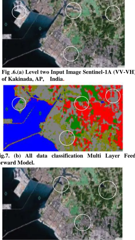
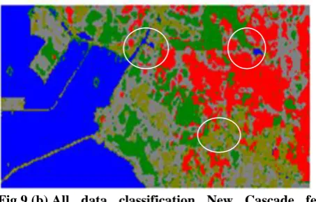
For each network, the input values are fed corresponding to different training classes, which are read into the networks that are trained. After training or learning, the pixel values are given as inputs for evaluation. The resultant images are depicted in this section (figures 6-8), whose base image is shown in fig. 6(a), 7(a) and 8(a). The results show that the random forest classifier has performed a little better classification than the Neural Network models delivered. Smaller regions which were misclassified by other Neural Networks were classified a little more accurately by random forest classifier. In figures 6(b) & 7(b), some variations in classifications given by MLFFNN and CFFNN are represented with white circles. The white circle in both figures 8 (a) and (b) represent the differences between the

input data and outputs and also its three techniques of SAR image classifications represents with white circles given by multilayer feed forward neural network, cascade forward neural network vis-à-vis Random Forest

Fig 5.Level one Sentinel-1A (VV-VH), (SAR Image) Input Image

Fig .6.(a) Level two Input Image Sentinel-1A (VV-VH) of Kakinada, AP, India.

Fig.7. (b) All data classification Multi Layer Feed forward Model.

[image:4.595.65.288.49.156.2] [image:4.595.312.534.95.211.2] [image:4.595.312.547.251.666.2]

(5)

Fig.9.(b).All data classification New Cascade feed forward NN

Fig.10.(a) Level two Input Image Sentinel-1A (VV-VH) of Kakinada, AP,India

Fig.11. (b) All data classification RF (Random Forest)

Water Bodies

Settlements

Forest

Vegetation

Open land

[image:5.595.50.284.36.549.2]

The class legend for all the classified outputs (figures 6-8) is common and given above.

Table.I. Classification methods and their Accuracy

S . N o

Individual Class Accuracy (%) Classificatio

n

Techniques Wat er Bod ies

Set tle me nts

Fo res t

Ve get ati on

Ope n Land 1 Multilayer

Feed forward

82 85 86 78 79

2 New Cascade Forward

83 86 89 76 86

3 Random Forest

[image:5.595.53.280.52.197.2] [image:5.595.318.538.55.228.2]

88 93 89 82 83

Table II. Overall Accuracy and Kappa Coefficient Classification

Algorithm

Overall Accuracy (%)

Kappa Coefficient Multilayer

Feed forward

82 0.766

New Cascade Forward

84 0.789

Random Forest

87 0.843

Table 1 describes class-wise accuracy of the thematic classes in the image and table 2 gives the overall accuracy and kappa coefficient. It is evident from the tables that the new cascade forward network fig 7(b) performed better than multi-layer feed forward network in classification of the image data of fig 6(b). Random Forest algorithm in fig 8(b) gave even better results than both the other methods. In Kakinada area, thematic regions are well connected and therefore the image data is amenable to good quality training sets. The authors are searching for more algorithms/techniques for achieving more accuracy.

IV. CONCLUSION

[image:5.595.49.283.237.492.2] [image:5.595.334.522.250.358.2] [image:5.595.66.196.522.686.2]

(6)

ACKNOWLEDGEMENTS

Authors would like to thank Dr. Rajashree Bothale, General Manager, Outreach Facility and Dr.Santanu Chowdhury, Director of National Remote Sensing Centre (ISRO), Hyderabad, NERTU and TEQIP-III of University College of Engineering Osmania University, Hyderabad, India, for their encouragement. The authors would also like to extend their sincere thanks to the institute staff for the invaluable support. The author would like to acknowledge CSIR, fellowship provided by Govt. of India. New Delhi, India which provided support for this work. The suggestions made by anonymous referees are gratefully acknowledged.

REFERENCES

1. Amitrano, D., Cecinati, F., Di Martino, G., Iodice, A., Mathieu, P.P., Riccio, 480 D., Ruello, G., 2018. Feature extraction from multi temporal SAR images 481 using self organizing map clustering and object-based image analysis. IEEE 482 Journal of Selected Topics in Applied Earth Observations and Remote Sensing .

2. Ma, X.; Liu, S.; Hu, S.; Geng, P.; Liu, M.; Zhao, J. SAR image edge detection via sparse representation. Soft Comput. 2017, doi:10.1007/s00500-017-2505-y

3. Muangnak N, Aimmanee P, Makhanov S (2017) Automatic optic disk detection in retinal images using hybrid vessel phase portrait analysis. Med Biol. Eng. Comput. https://doi.org/10.1007/s11517-017-1705-z. 4. Otto, D. Wang and A. K. Jain “Clustering Millions of Faces by Identity”

arXiv:1604.00989, 2016

5. Depizzol, D.B., Montalv~ao, J., Lima, F.d.O., et al. Feature selection for optical network design via a new mutual information estimator", Expert Systems with Applications, 107, pp. 72-88 (2018).

6. Novoa J, Chokmani K and Lhissou R 2018 A novel index for assessment of riparian strip efficiency in agricultural landscapes using high spatial resolution satellite imagery Science of The Total Environment 644 1439–51.

7. B. Zhang, J. Gu, C. Chen, J. Han, X. Su, X. Cao, and J. Liu. One-two-one network for compression artifacts reduction in remote sensing. ISPRS Journal of Photogrammetry and Remote Sensing, 2018. 8. Ni, G., Moser, G., Wray, N. R. & Lee, S. H. Estimation of genetic correlation using linkage disequilibrium score regression and genomic restricted maximum likelihood. American Journal of Human Genetics 102, 1185–1194 (2018).

9. Rostami A., Anbaz M.A., Gahrooei H.R.E., Arabloo M., Bahadori A. (2017) Accurate estimation of CO 2 adsorption on activated carbon with multi-layer feed-forward neural network (MLFNN) algorithm, Egypt. J. Petrol. doi:10.1016/ j.ejpe.2017.01.003

10. Ansari HR, Zarei MJ, Sabbaghi S, Keshavarz P (2018) A new comprehensive model for relative viscosity of various nanofluids using feed-forward back-propagation MLP neural networks. IntCommun Heat Mass 91:158–164.

11. Zou, W., Yao, F., Zhang, B., & Guan, Z. (2018). Back Propagation Convex Extreme Learning Machine. In Proceedings of ELM-2016 (pp. 259-272). Springer, Cham.

12. Sumit Goyal and Gyandera Kumar Goyal Cascade and Feedforward Backpropagation Artificial Neural Network Models For Prediction of Sensory Quality of Instant Coffee Flavoured Sterilized Drink. Canadian Journal on Artificial Intelligence, Machine Learning and Pattern Recognition Vol. 2, No. 6, August 2011

13. Zhu, M.; Xia, J.; Jin, X.; Yan, M.; Cai, G.; Yan, J.; Ning, G. Class Weights Random Forest Algorithm for Processing Class Imbalanced Medical Data. IEEE Access 2018, 6, 4641–4652.

14. C.H. Chen, “Signal and Image Processing for Remote Sensing”, CRC publ., Taylor & Francis, 2011, pp. 328 – 329

AUTHORS PROFILE

Battula Balnarsaiah received from B. Tech and M. Tech degrees in Electronics and Communication Engineering from Jawaharlal Nehru Technology University Hyderabad (JNTU-H), India, in 2003 and 2012, respectively. He is currently pursuing research at Research and Training Unit for Navigational Electronics (NERTU), Dept of ECE, and

University College of Engineering in Osmania University. His research interest areas are Image Processing, Synthetic Aperture Radar (SAR) Images and Machine Learning, Deep Learning. Three of his papers were published international conferences viz., one in IEEE Explore and other two are in Springer. He has IEEE membership

T.S. Prasad holds M.Sc. Physics, M. Tech Remote Sensing and Advanced Level Course in Computer Science degrees. He has experience in teaching of basics of Remote Sensing, Digital Image Processing, Pattern Recognition, fundamentals of Microwave Remote Sensing, Neural Networks and Geographic Information Systems and project experience in the said fields. He has flair for software writing and has written software for Pattern Classification of Satellite Imagery and Soil Moisture estimation from satellite Microwave Remote Sensing data which gave worthy results. He has publications in national conferences and International Journals and conferences.