Simon Mizzi
12∗, David R. Emerson
2, Stefan K. Stefanov
3,
Robert W. Barber
2, and Jason M. Reese
11Department of Mechanical Engineering, University of Strathclyde, Glasgow G11XJ, United Kingdom 2Centre for Microfluidics and Microsystems Modelling, CCLRC Daresbury Laboratory,
Warrington WA4 4AD, United Kingdom
3Institute of Mechanics, Bulgarian Academy of Sciences, Acad. G. Bonchev Str., Bl. 4, Sofia 1113, Bulgaria
The Navier-Stokes-Fourier equations, with boundary conditions that account for the effects of velocity-slip and temperature-jump, are compared to the direct simulation Monte Carlo method for the case of a lid-driven micro-cavity.Results are presented for Knudsen numbers within the slip-flow regime where the onset of nonequilibrium effects are usually observed.Good agreement is found in predicting the general features of the velocity field and the recirculating flow.However, although the steady-state pressure distributions along the walls of the driven cavity are generally in good agreement with the Monte Carlo data, there is some indication that the results are starting to show noticeable differences, particularly at the separation and reattachment points.The modi-fied Navier-Stokes-Fourier equations consistently overpredict the maximum and minimum pressure values throughout the slip-regime.This highlights the need for alternative boundary formulations or modeling techniques that can provide accurate and computationally economic solutions over a wider range of Knudsen numbers.
Keywords:
Microfluidics, Cavity Flow, Slip-Regime, Non-Equilibrium Phenomena, Knudsen Number.1. INTRODUCTION
The use of micro-electro-mechanical systems (MEMS) has been proposed in many applications, including industrial engineering, biomedical analyses, environmental control, micro-processor cooling and high-precision printing.As a result, terms such as micro-ducts, micro-heat-exchangers, micro-pumps, and micro-sensors are now commonly used in many diverse fields.One area where the research com-munity is particularly active is trying to understand gas dynamics in micron and sub-micron sized domains.The flow characteristics in miniaturized systems are known to differ significantly from those found in conventional devices.For example, the Navier-Stokes-Fourier (NSF) equations with no-slip boundary conditions are no longer valid when the characteristic length scale enters the micron range.1
The inadequacy of the NSF equations in modeling gas dynamics in micron-sized domains can be explained by the fact that they are only able to describe flows that are close to thermodynamic equilibrium.However, at small length scales, nonequilibrium effects are frequently observed in
∗Author to whom correspondence should be addressed.
gas flows.Collisions between the molecules are the only mechanism for a gas to maintain equilibrium.If a gas is too rarefied or confined in a micro-geometry, the number of intermolecular collisions will be significantly reduced and nonequilibrium effects will start to dominate.The degree of rarefaction of a gas is defined through the Knudsen number, Kn, which is given by Kn=/L, where is the mean free path (i.e. the average distance travelled by the gas molecules between successive collisions) andL is the characteristic size of the domain.
2. MODELING APPROACHES
The Boltzmann equation is the fundamental governing equation for a dilute gas undergoing binary collisions.The basic form of the Boltzmann equation can be written as
f t +ci
f xi
+ai
f ci
=f
t
C
(1) where f is the particle distribution function which is a function of time,t, the position vector,xi, and the molec-ular velocity vector, ci.The term on the right-hand side
of Eq.(1), f /tC, is a production term for f resulting
from the binary collisions and is commonly referred to as thecollision operator.The Boltzmann equation is able to describe gases that are in equilibrium and nonequilibrium alike but its solution is a non-trivial task due to the com-plexity of the collision term.
Various methods have been proposed to simplify Eq.(1) with each method attempting to retain an acceptable level of accuracy in describing the fundamental physics.There are essentially two main approaches for simulating rar-efied gases; in one approach, discrete molecular modeling is used to describe the fluid through a microscopic for-malism, i.e. as a collection of moving molecules which interact through collisions or very close proximity poten-tials.Discrete modeling can be performed using either statistical ensemble averages, as in the direct simulation Monte Carlo approach,2 or through deterministic
meth-ods, such as molecular dynamics.3Although discrete
meth-ods achieve a realistic representation of the microscopic behavior, their application has been restricted to geomet-rically simple flows due to their computationally inten-sive nature.4 However, the information preservation (IP)
method56may offer a promising approach for reducing the
computational requirements of DSMC techniques while Baker and Hadjiconstantinou7 have recently demonstrated
that the statistical scatter associated with Monte Carlo methods can be reduced by considering only the deviation from the equilibrium condition.
An alternative approach is to retain a continuum formu-lation to develop simpler representations of the Boltzmann equation.In this case, the fluid is assumed to be continu-ous and infinitely divisible so that velocity, density, pres-sure, and other properties can readily be defined at any point in space and time.One such approach is through the use of an extended hydrodynamic approximation of Eq.(1).This can be obtained by performing a Chapman-Enskog expansion,8 where the distribution function, f, is
expanded in a power series based on the Knudsen number. The power series can be truncated at any power of Kn and will yield the Euler, NSF, Burnett, or higher-order descrip-tions.Another approach is the method of moments9–11
where the distribution function is multiplied by a function that depends only on the molecular velocity.The transport equations can then be derived from a power series involv-ing Hermite polynomials.It should be noted that there are
a number of challenges with the foregoing approaches.For example, the Burnett equations have stability issues and are unable to capture Knudsen layers whilst moment meth-ods do not provide a closed system and also require addi-tional boundary conditions.However, there are advantages in these approaches because they are globally second-order (or higher) in Knudsen number and will naturally recover the NSF equations when the Knudsen number is small.
Alternatively, it is possible to combine the NSF equa-tions with simple phenomenological extensions.Such techniques include the application of velocity-slip12 and
temperature-jump13 boundary conditions.It is also
possi-ble to develop second-order boundary conditions for the velocity-slip1415or to derive more accurate boundary
con-ditions based on higher-order constitutive relations, such as the Burnett equations.16 These techniques improve the
accuracy of mass flow rate predictions but often fail to cap-ture nonlinear phenomena in the near-wall region.More recently, the development of constitutive law re-scaling, in the form of a wall function,17has been shown to offer the
potential of replicating the nonlinear stress/strain behav-ior in the vicinity of solid walls.For the present analysis, we use a boundary formulation derived from Grad’s 13 moment equations.11
3. CLASSIFICATION OF THE FLOW REGIME
Several distinct regimes can be defined that characterize the state of a particular flow:1
• For Kn<0001, the flow is in thecontinuum regimeand the conventional no-slip boundary condition is considered to be valid since the flow is in thermodynamic equilibrium. • For 0001<Kn<01, the gas is in theslip-flow regime. The NSF equations are considered to be adequate provided the effects of velocity-slip and temperature-jump at the wall are taken into account.
• For 01<Kn<10, the flow is said to be in the transi-tion regime.The use of the NSF equations becomes ques-tionable and alternative approaches are needed to model such flows using either discrete (particle-based) methods, extended hydrodynamics, or the method of moments. • For Kn>10, the flow is in thefree-molecular regime.In this regime, the frequency of intermolecular collisions is very low and the mean free path is large compared to the characteristic length scale of the flow domain.The con-tinuum hypothesis is no longer valid and a collisionless form of the Boltzmann equation can be used to describe the flow.
The limiting Knudsen numbers in the above classifica-tion scheme are somewhat empirical, and are generally based upon simple flows that have a predominant flow direction and pronounced gradients normal to the stream-wise direction, e.g., Couette or Poiseuille flow. In the case of more complex flows, however, the boundaries between the different regimes may depend upon the particular geometric details of the problem.As will be demonstrated
later for a driven-cavity flow, nonequilibrium effects are discernible at Knudsen numbers well below the conven-tionally accepted upper limit of the slip-flow regime.
4. THE DRIVEN CAVITY PROBLEM
Cavities, steps and cut-outs occur frequently in many engineering designs.Such configurations generate sharp changes in the flow variables and their gradients.At the macroscopic scale, modeling the flow phenomena asso-ciated with cavities is challenging, particularly at high Mach numbers.However, at the microscale, other com-plexities can arise due to the loss of local thermodynamic equilibrium.
The lid-driven cavity, shown schematically in Figure 1, has been extensively investigated in a completely differ-ent context since the problem is often used as a validation test for numerical schemes.Despite its geometric simplic-ity, the problem is rich in flow physics associated with the recirculating eddy.Many of the investigations in the liter-ature are presented in an incompressible NSF framework and are solved using either a pressure–velocity coupling or a streamfunction-vorticity formulation.1819 In general,
the objective of these studies is to investigate the effective-ness of convective numerical schemes over a wide range of Reynolds numbers.
In the present paper, we investigate a micro-scale lid-driven cavity since very few studies are available for rar-efied cavity flows.Su et al.20 presented solutions obtained
using the Bhatannagar-Gross-Krook (BGK) approximation of the Boltzmann equation while Jiang et al.21 compared
the DSMC and information preservation (IP) methods, and investigated the validity of the IP method for low-speed flows.More recently, Naris and Valougeorgis22 have
con-ducted a comprehensive study of the driven cavity prob-lem over the whole Knudsen number regime using the discrete velocity method to solve the linearized Boltzmann equation.They showed that for low Mach number flows,
D A
[image:3.728.93.254.528.711.2]B C
Fig. 1. Schematic diagram of a driven cavity.
the temperature variations were small.In the present study, we compare NSF predictions with results obtained from the DSMC method.In particular, we highlight some of the limitations of the NSF approach in the slip-flow regime.
5. NUMERICAL SOLUTION OF THE
NSF EQUATIONS
The Navier-Stokes-Fourier equations have been discretized on a collocated grid using the finite-volume pressure-velocity-density coupling approach proposed by Demirdzic et al.23 Since the Reynolds number is relatively small, a
central-difference scheme is considered appropriate.24The
central-difference scheme was implemented at cell bound-aries for both the convective and diffusive fluxes while the source terms were computed at cell centres.A mesh-resolution study was carried out using grids composed of 40×40, 80×80 and 160×160 cells.In all test cases, the results were numerically equivalent for the 80×80 and 160×160 grids.We present here only the grid-independent results.
5.1. Velocity-Slip and Temperature-Jump Boundary Conditions
The application of velocity-slip and temperature-jump boundary conditions in the NSF equations is a simpli-fied phenomenological approach to represent both non-equilibrium and gas-surface interaction effects near the solid walls.These boundary conditions were first proposed by Maxwell12 and von Smoluchowski,13 respectively.
Using Grad’s closure approximation for the distribution function,f, the boundary conditions can be written as:11
vislip=vigas−viwall
=−2− /
2
√
RT 1ijnj−nijknjnk−
1
52qi−niqknk
RT+1 2jknjnk
(2)
and Twall
T −1 =2−T/T
2RT 1
21qknk+14jknjnk
p+1 2jknjnk
−vi4RTslipvislip (3)
wherevislip is the slip velocity at the wall,vigas andviwall are the gas and wall velocities,TwallandT are the wall and gas
temperatures, andT are the tangential momentum and
energy accommodation coefficients, respectively, and ij andqiare the viscous stresses and heat flux.The term,ni,
is the normal vector,pis the pressure,is the density, and R is the specific gas constant.The terms, 1,2, and 1 are Knudsen layer correction coefficients and are set to 1 = 1114, 2 = 134533, and 1 = 1127,
respectively11 while the tangential momentum and energy
6. DIRECT SIMULATION MONTE CARLO
SOLUTION
The DSMC method used in this study follows the approach proposed by Bird2where the gas molecules are represented
by a much smaller number of “stochastic” particles.The algorithm is divided into two main stages consisting of translational movement of the particles and binary colli-sions between the particles.Solid boundaries are taken into account in the translational stage of the algorithm and a special recursive treatment is implemented in the vicinity of the corners of the cavity.A Maxwellian scattering ker-nel with perfect accommodation is assumed at the walls and the “no time counter” method is used to simulate the collision interactions.
In the present paper, we are interested in the steady-state solution.Since the DSMC method is a kinetic for-mulation (i.e. dependent on time, molecular velocity, and position), the macroscopic variables are computed using time-averaged moments over a number of kinetic time steps.The moments are spatially averaged within the cell volumes.In particular, we have computed the following moments:m,mc¯i,mcici/2,mCiCj, andmCiCiCj/2 where
m is the molecular mass and Ci is the peculiar
veloc-ity defined as the deviation of the molecular velocveloc-ity, ci,
from the average velocityui (i.e.Ci=ci−ui), the overbar
indicates time-averaged values and repeated indices rep-resent the usual Einstein convention of tensor summation. These averages yield moments corresponding to the den-sity, bulk velocity, internal energy, viscous stress, and heat flux, respectively.
The DSMC simulations employed a hard-sphere model of argon with a molecular mass of 663×10−26 kg and
a molecular diameter of 342×10−10 m.The
computa-tional domain was discretized using a uniform distribution of cells with a grid resolution of either 50×50 or 60×60 cells, depending upon the Knudsen number.Typically, the DSMC simulations employed 50 particles per cell although this was increased to approximately 300 particles per cell for the lowest Knudsen number case.Over 10 million sam-pling time steps were used to reduce the statistical scatter in the DSMC results.
7. RESULTS AND DISCUSSION
The lid-driven cavity has been investigated for two Knudsen numbers, Kn=005 and Kn=01.For conve-nience, the results are presented in a nondimensional form given by the following:
X=x1
L Y = x2
L S= s
L P = p Po
U = v1 Ulid
and V= v2 Ulid
(4) wherex1 andx2 are the horizontal and vertical distances,
respectively,Lis the cavity length,sis the distance along
(a)
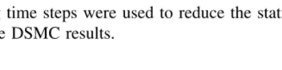
[image:4.728.94.293.649.698.2](b)
Fig. 2. Velocity streamlines for Kn=005: (a) NSF solution and (b) DSMC data.
the walls of the cavity (starting fromAin Fig.1 and pro-gressing in a clockwise direction), Po is the initial
pres-sure in the cavity (Po=101135 N m−2),v1andv2 are the
velocity components in thex1andx2directions, andUlidis
the velocity of the moving wall.The upper case symbols represent the nondimensional quantities.
Figures 2 and 3 compare the streamlines predicted by the NSF and DSMC approaches at the two Knudsen num-bers.The simulations have considered a driven cavity with a unit aspect ratio.In both cases, the Mach number, defined as Ma=Ulid/
2RT0, where T0 is the reference
tempera-ture (273 K), was 0.09. In general, the agreement between the two modeling approaches is very good and the NSF equations predict the overall features of the flow with rea-sonable accuracy, including the location of the centre of the eddy.Figure 4 compares the predicted velocity pro-files along the centreline of the cavity (x1/L=05 and x2/L=05).Once again, the two modeling approaches yield very similar results but the NSF equations overpre-dict the velocity-slip along the moving wall at Kn=01.
(a)
[image:5.728.59.288.63.446.2](b)
Fig. 3. Velocity streamlines for Kn=01: (a) NSF solution and (b) DSMC data.
In the cases considered, the flow field consists of a single primary recirculating eddy with the flow having insuffi-cient inertia to generate secondary vortices in the corners of the cavity.
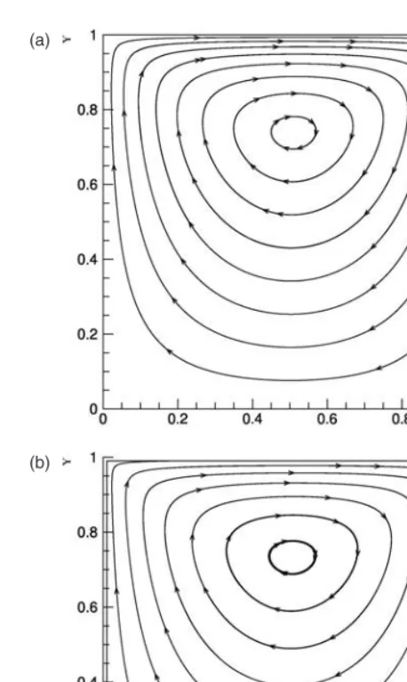
Figure 5 shows the nondimensional pressure distribution along the walls of the cavity.For both Knudsen numbers, it can be seen that there is reasonable agreement between the NSF solution and the DSMC predictions.However, in both cases, the NSF predictions show considerable discrepan-cies in the vicinity of the uppersrleft-hand and right-hand corners of the cavity (S=1 and S=2), where separa-tion and reattachment occur.The DSMC predicsepara-tions are very similiar to the pressure distributions obtained by Jiang et al.21 In contrast, the NSF equations overestimate the
pressure difference between these two corner points (B and C in Figure 1) leading to an incorrect pressure distribution along the moving wall of the cavity.The accurate predic-tion of reattachment pressures is particularly important and the present results show that, for the driven cavity prob-lem, nonequilibrium effects are causing inaccuracies well
(a)
[image:5.728.317.540.64.456.2](b)
Fig. 4. Velocity profiles along the centreline of the cavity (x1/L=05
andx2/L=05): (a) Kn=005 and (b) Kn=01.Comparison of DSMC
data (•) and the NSF solution (—).
before the conventionally-accepted upper limit of the slip-flow regime.
8. CONCLUSIONS
(a)
(b)
4 3
2 1
0 0.8 0.9 1.1 1.2 0.8 0.9 1.1
1 1.2
PP
S 4 3
2 1
0
S
B A
A D
C B
D
A A
[image:6.728.60.288.63.433.2]C
Fig. 5. Pressure distribution along the cavity walls: (a) Kn=005 and (b) Kn=01.Comparison of DSMC data (•) and the NSF solution (—).
alternative boundary treatments or modeling approaches that can provide accurate and computationally economic solutions over a wider range of Knudsen numbers.
Acknowledgments: The authors are grateful to the
UK Engineering and Physical Sciences Research Coun-cil (EPSRC) for supporting this research under Grant
No.GR/S77196/01.Additional support was provided by EPSRC under the auspices of Collaborative Computational Project 12 (CCP12).
References
1. M.Gad-el-Hak,ASME J. Fluids Engrg.121, 5(1999).
2. G.A.Bird, Molecular Gas Dynamics and the Direct Simulation of Gas Flows, Clarendon Press, Oxford(19945).
3. D.C.Rapaport, The Art of Molecular Dynamics Simulation, Cambridge University Press, Cambridge, UK(2004).
4. E.S.Oran, C.K.Oh, and B.Z.Cybyk,Ann. Rev. Fluid Mechanics
30, 403(1998).
5. J.Fan and C.Shen,J. Computational Phys.167, 393(2001).
6. Q.Sun and I.D.Boyd, Theoretical development of the information preservation method for strongly nonequilibrium flows.Proceedings of the 38th Thermophysics Conference, Toronto, Canada(2005).
7. L.L.Baker and N.G.Hadjiconstantinou, Physics of Fluids 17, 051703(2005).
8. S.Chapman and T.G.Cowling, The Mathematical Theory of Non-Uniform Gases, Cambridge University Press, Cambridge, UK
(1990).
9. H.Grad,Commun. Pure Appl. Math.2, 331(1949).
10. M.N.Kogan, Rarefied Gas Dynamics, Plenum Press, New York
(1969).
11. H.Struchtrup, Macroscopic Transport Equations for Rarefied Gas Flows, Springer, Germany(2005).
12. J.C.Maxwell,Philos. Trans. R. Soc. London170, 231(1879).
13. M.von Smoluchowski, Annalen der Physik und Chemie 64, 101
(1898).
14. N.G.Hadjiconstantinou,Physics of Fluids15, 2352(2003).
15. R.W.Barber and D.R.Emerson,Heat Transfer Engrg.27, 3(2006).
16. D.A.Lockerby, J.M.Reese, D.R.Emerson, and R.W.Barber,
Phys. Rev. E70, 017303(2004).
17. D.A.Lockerby, J.M.Reese, and M.A.Gallis,AIAA J.43, 1391
(2005).
18. P.N.Shankar and M.D.Deshpande,Ann. Rev. Fluid Mech.32, 93
(2000).
19. E.Erturk, T.C.Corke, and C.Gökcöl,Int. J. Numer. Meth. Fluids
48, 747(2005).
20. M.Su, K.Xu, and M.S.Ghidaoui,J. Computational Phys.150, 17
(1999).
21. J.Jiang, J.Fan,and C.Shen,AIPConference Proceedings – Rarefied Gas Dynamics: 23rd International Symposium (2003), Vol.663, p.784.
22. S.Naris and D.Valougeorgis,Physics of Fluids17, 097106(2005).
23. I.Demirdzic, Z.Lilek, and M.Peric,Int. J. Numer. Meth. Fluids16, 1029(1993).
24. J.H.Ferziger and M.Peric, Computational Methods for Fluid Dynamics, Springer-Verlag, Germany(19965666).
Received: 4 October 2006.Accepted: 23 October 2006.