modelling of 15 systems
.
White Rose Research Online URL for this paper:
http://eprints.whiterose.ac.uk/144934/
Version: Accepted Version
Article:
McAllister, M., Littlefair, S.P., Parsons, S.G. et al. (13 more authors) (2019) The
evolutionary status of Cataclysmic Variables: Eclipse modelling of 15 systems. Monthly
Notices of the Royal Astronomical Society. ISSN 0035-8711
https://doi.org/10.1093/mnras/stz976
This is a pre-copyedited, author-produced PDF of an article accepted for publication in
Monthly Notices of the Royal Astronomical Society following peer review. The version of
record M McAllister, S P Littlefair, S G Parsons, V S Dhillon, T R Marsh, B T Gaensicke, E
Breedt, C Copperwheat, M J Green, C Knigge, D I Sahman, Martin J Dyer, P Kerry, R P
Ashley, P Irawati, S Rattanasoon, The evolutionary status of Cataclysmic Variables:
Eclipse modelling of 15 systems, Monthly Notices of the Royal Astronomical Society is
available online at: https://doi.org/10.1093/mnras/stz976.
[email protected]
https://eprints.whiterose.ac.uk/
Reuse
Items deposited in White Rose Research Online are protected by copyright, with all rights reserved unless
indicated otherwise. They may be downloaded and/or printed for private study, or other acts as permitted by
national copyright laws. The publisher or other rights holders may allow further reproduction and re-use of
the full text version. This is indicated by the licence information on the White Rose Research Online record
for the item.
Takedown
If you consider content in White Rose Research Online to be in breach of UK law, please notify us by
The evolutionary status of Cataclysmic Variables: Eclipse
modelling of 15 systems.
M. McAllister
1
, S. P. Littlefair
1
, S. G. Parsons
1
, V. S. Dhillon
1
,
2
, T. R. Marsh
3
B. T. G¨
ansicke
3
, E. Breedt
4
, C. Copperwheat
5
, M. J. Green
3
, C. Knigge
6
D. I. Sahman
1
, Martin J. Dyer
1
, P. Kerry
1
, R. P. Ashley
3
, P. Irawati
7
, S. Rattanasoon
7
1Dept of Physics and Astronomy, University of Sheffield, Sheffield, S3 7RH, UK2Instituto de Astrof´ısica de Canarias (IAC), E-38200, La Laguna, Tenerife, Spain 3Dept of Physics, University of Warwick, Coventry, CV4 7AL, UK
4Institute of Astronomy, University of Cambridge, Madingley Road, Cambridge, CB3 0HA, UK
5Astrophysics Research Institute, Liverpool John Moores University, IC2, Liverpool Science Park, L3 5RF, UK 6School of Physics & Astronomy, University of Southampton, Southampton SO17 1BJ, UK
7National Astronomical Research Institute of Thailand, 191 Siriphanich Bldg., Huay Kaew Road, Chiang Mai 50200, Thailand
Accepted XXX. Received YYY; in original form ZZZ
ABSTRACT
We present measurements of the component masses in 15 Cataclysmic Variables (CVs) - 6 new estimates and 9 improved estimates. We provide new calibrations of the relationship between su-perhump period excess and mass ratio, and use this relation to estimate donor star masses for 225 superhumping CVs. With an increased sample of donor masses we revisit the implications for CV evolution. We confirm the high mass of white dwarfs in CVs, but find no trend in white dwarf mass with orbital period. We argue for a revision in the location of the orbital period minimum of CVs to 79.6±0.2min, significantly shorter than previous estimates. We find that CV donors below the gap have an intrinsic scatter of only 0.005 R⊙ around a common evolutionary track, implying a
corre-spondingly small variation in angular momentum loss rates. In contrast to prior studies, we find that standard CV evolutionary tracks - without additional angular momentum loss - are a reasonable fit to the donor masses just below the period gap, but that they do not reproduce the observed period minimum, or fit the donor radii below 0.1 M⊙.
Key words: binaries: close – binaries: eclipsing – stars: evolution – novae, cataclysmic
variables – white dwarfs – stars: dwarf novae
1 INTRODUCTION
Cataclysmic Variables (CVs) are close binary stars in which a white dwarf is accreting material from a low-mass donor star. Without angular momentum loss (AML) from the sys-tem, mass transfer could not be sustained; thus it is the AML that drives the secular evolution of CVs. The currently ac-cepted picture of CV evolution is that CVs evolve from long to short periods under the influence of AML caused by mag-netic braking. A reduction in AML due to magmag-netic braking is thought to arise when the donor becomes fully convective. This causes the CV to become detached, and is the cause of the dearth of CVs in the 2–3 hour orbital period range; the CVperiod gap. When the CV resumes mass transfer, AML is driven by gravitational radiation and the mass transfer rate is lower. The CV evolves slowly through aperiod minimum, which arises because the thermal timescale of the donor be-comes comparable to the mass loss timescale, and the donor begins to expand in response to mass loss, which leads to a widening of the orbit.
This long-standing picture has survived for over 35 years
(Rappaport et al. 1982,1983) despite the fact that it
strug-gles to explain the observed value of the period minimum
(G¨ansicke et al. 2009), the scarcity of known
post-period-minimum systems (Hern´andez Santisteban et al. 2018) and the average high white dwarf mass in CVs (Zorotovic et al. 2011). Modifications to the standard model exist that can potentially explain some of these issues. The orbital period minimum problem can be solved with an additional source of AML for short period systems (Patterson 1998;Knigge et al. 2011), and AML in nova outbursts may cause CVs with low-mass white dwarfs to be unstable, explaining the high aver-age white dwarf mass (Schreiber et al. 2016;Nelemans et al. 2016). However, it remains to be seen if those modifications can correctly describe the observed properties of known CVs. In particular, the mass and radius of the donor star is a sen-sitive probe of the secular evolution. This is because the radius of the donor star in a CV can be inflated from the main-sequence value, by some amount that depends upon
D
o
w
n
lo
a
d
e
d
fro
m
h
ttp
s:
//a
ca
d
e
mi
c.
o
u
p
.co
m/
mn
ra
s/
a
d
va
n
ce
-a
rt
icl
e
-a
b
st
ra
ct
/d
o
i/1
0
.1
0
9
3
/mn
ra
s/
st
z9
7
6
/5
4
7
9
2
5
5
b
y
U
n
ive
rsi
ty
o
f S
h
e
ffi
e
ld
u
se
r
o
n
2
5
A
p
ri
l 2
0
1
the mass-loss history of the donor. In particular, the donor radius is more likely to track the long-term average mass loss rate than other physical properties of the CV such as the accretion light or the effective temperature of the ac-creting white dwarf (see Knigge et al. 2011, and references within).
One of the best methods of measuring donor masses and radii is to model the primary eclipse. During primary eclipse, the white dwarf and accretion disc are occulted, along with the bright spot, located where the accretion stream impacts the outer rim of the disc. The path of the gas stream is determined by the mass ratio, and so the detailed shape of the primary eclipse contains enough information to de-rive extremely precise masses that are consistent with con-ventional spectroscopic methods (see Tulloch et al. 2009;
Copperwheat et al. 2010;Savoury et al. 2012, for example).
The photometric method has the advantage that it does not rely on detection of the light from the donor star, which is of-ten invisible given the much brighter white dwarf and accre-tion disc, particularly for CVs with shorter orbital periods. It does however require high quality lightcurves of the eclipses, which occur on timescales of minutes. With this in mind, our group has been acquiring high quality lightcurves of eclips-ing CVs with the high time-resolution instruments ULTRA-CAM (Dhillon et al. 2007) and ULTRASPEC (Dhillon et al. 2014). Here we present the analysis of 15 systems, and re-view the evolutionary status of CV systems in light of the results.
1.1 Systems selected for eclipse modelling
The 15 systems modelled in this paper are listed in Ta-ble 1. CTCV 1300, DV UMa, SDSS 1152, SDSS 1501 have existing mass determination from eclipse modelling of ULTRACAM data (Savoury et al. 2011), whilst Z Cha, OY Car, IY UMa, GY Cnc and SDSS 1006 have ex-isting mass determinations in the literature from var-ious methods (Wood et al. 1986; Wade & Horne 1988;
Wood & Horne 1990;Thorstensen 2000;Steeghs et al. 2003;
Southworth et al. 2009; Copperwheat et al. 2012). The
ex-isting mass determinations have large associated errors, and we re-analyse them here in the light of new data, and an up-dated modelling approach (see McAllister et al. 2017a, for details). The remaining 6 systems have no existing donor mass estimates, and were chosen from the eclipsing CVs ob-served with ULTRACAM/ULTRASPEC to date; the pri-mary reason for their selection was an eclipse shape suit-able for modelling, with visible white dwarf and bright spot eclipses.
2 OBSERVATIONS AND DATA REDUCTION
The observations in this paper span a range of dates from May 2003 to Feb 2017. All data were taken with the triple-band fast camera ULTRACAM, or the single-triple-band fast cam-era ULTRASPEC. ULTRACAM data were taken on three telescopes; the 4.2-m William Herschel Telescope (WHT) situated at the Roque de los Muchachos Observatory on La Palma, Spain, the 8.2-m Very Large Telescope (VLT) at Paranal, Chile, and the 3.5-m New Technology Telescope (NTT) located at La Silla, Chile. All ULTRASPEC data
were taken using the 2.4-m Thai National Telescope (TNT), located on Doi Inthanon in Thailand. All observations were obtained using the Sloan Digital Sky Survey (SDSS) filter set, with the exception of some of the ULTRASPEC obser-vations, which use the KG5 filter. This filter is described in detail inHardy et al.(2017); it is a broadband filter encom-passing the SDSSu′,
g′ andr′passbands. For a full journal
of observations, see TableC1.
Data reduction was carried out using the ULTRACAM pipeline reduction software (seeDhillon et al. 2007). One or more nearby, photometrically stable comparison stars were used to correct for transparency variations during observa-tions. If the comparison stars have tabulated SDSS magni-tudes, we used these to transform the photometry into the
u′
g′r′i′z′ standard system (Smith et al. 2002), otherwise
observations of standard stars from the nearest photometric night were used. Photometry was corrected for extinction using the median extinction coefficients for each observa-tory, as derived from long duration time-series taken with ULTRACAM and ULTRASPEC.
3 METHODS
3.1 Orbital Ephemerides
Updated orbital ephemerides for the CVs in this paper were calculated, and are shown in Table1. Mid-eclipse times were determined by averaging the time of white dwarf ingress and egress, as determined by locating the minima and maxima of a smoothed lightcurve derivative. Mid eclipse times were cor-rected to the Solar System Heliocentre or Barycentre using
astropy(The Astropy Collaboration et al. 2018). The
cor-rection used was decided upon a system-to-system basis, and depended on previous mid-eclipse times and ephemerides in the literature. Heliocentric times are recorded in Coordi-nated Universal Time (UTC), Barycentric times in Barycen-tric Dynamical Time (TDB). Mid-eclipse times for each in-dividual eclipse observed are presented in TableC1.
3.2 Eclipse light-curve modelling
The model used to fit the eclipse light curve is described
bySavoury et al.(2011). The important assumptions in the
model are that the bright spot lies on the ballistic trajec-tory from the donor, the white dwarf follows a theoretical mass-radius relation and that the white dwarf is unobscured. The model has recently received two major improvements, as outlined inMcAllister et al.(2017a). The model now has the ability to fit multiple lightcurves simultaneously whilst sharing parameters that do not change; such as the mass ra-tioq, the white dwarf eclipse width∆Φand the white dwarf radius, scaled by the binary separation R1/a. In addition, the model now has a statistical treatment of flickering using Gaussian Processes (GPs) that makes the uncertainty esti-mates for these parameter robust in the presence of flicker-ing. For each system we either fit all the individual eclipses, or averaged several eclipses in the same filter. Averaging eclipses can ease convergence of the model, by reducing the number of free parameters, but it is not suitable when the lightcurve features change between eclipses, for example due to a changing accretion disc radius.
D
o
w
n
lo
a
d
e
d
fro
m
h
ttp
s:
//a
ca
d
e
mi
c.
o
u
p
.co
m/
mn
ra
s/
a
d
va
n
ce
-a
rt
icl
e
-a
b
st
ra
ct
/d
o
i/1
0
.1
0
9
3
/mn
ra
s/
st
z9
7
6
/5
4
7
9
2
5
5
b
y
U
n
ive
rsi
ty
o
f S
h
e
ffi
e
ld
u
se
r
o
n
2
5
A
p
ri
l 2
0
1
Object Right Declination Out-of eclipse Mag. T0 Porb Necl Add. Ecl.
Ascension (g′) (MJD) (d) Times
CTCV J1300−3052 13 00 29.05 −30 52 57.1 18.6 54262.099166(18)h 0.0889406998(17) 4 1 DV UMa 09 46 36.65 +44 46 45.1 18.7 52782.973948(10)h
0.0858526308(7) 4 2,3,4 SDSS J115207.00+404947.8 11 52 07.01 +40 49 48.0 19.5 55204.101279(6)h
0.0677497026(3) 7 5 SDSS J150137.22+550123.4 15 01 37.24 +55 01 23.5 19.0 56178.870444(8)h
0.05684126603(21) 12 – CSS080623 J140454−102702 14 04 53.97 −10 27 02.3 19.5 55329.234631(13)h 0.059578971(3) 10 – CSS110113 J043112−031452 04 31 12.45 −03 14 51.6 19.5 55942.014642(15)h 0.0660508707(18) 12 – GY Cnc 09 09 50.55 +18 49 47.5 16.7 55938.263734(22)b
0.175442399(6) 12 – IY UMa 10 43 56.73 +58 07 31.9 17.1 56746.6395010(9)h
0.07390892818(21) 10 8 OY Car 10 06 22.07 −70 14 04.6 15.6 55353.996477(3)h 0.06312092545(24) 7 – SDSS J090103.94+480911.0 09 01 03.94 +48 09 11.0 19.5 55942.116358(8)h
0.0778805321(5) 10 9 SDSS J100658.40+233724.4 10 06 58.42 +23 37 24.6 18.6 56682.72973(5)h
0.185913107(13) 11 7,10 SSS130413 J094551−194402 09 45 51.00 −19 44 00.8 16.7 56683.673971(12)h 0.0657692903(12) 17 6 SSS100615 J200331−284941 20 03 31.27 -28 49 41.3 19.6 56873.023625(5)h 0.0587045(4) 3 – V713 Cep 20 46 38.70 +60 38 02.8 18.5 56176.936402(7)h
0.0854185080(12) 15 11 Z Cha 08 07 27.75 −76 32 00.7 15.6 53498.011471(4)h 0.0744992631(3) 14 –
Table 1.Ephemerides for the CVs modelled in this paper.T0is the mid-eclipse time of cycle 0,Porb is the orbital period, while Necl
is the total number of eclipses obtained. References for additional eclipse times: (1)Tappert et al.(2004), (2)Howell et al. (1988), (3)
Patterson et al.(2000), (4)Nogami et al.(2001), (5)Southworth et al.(2010), (6)Thorstensen et al.(2016), (7) Woudt (priv. comm.),
(8) Coppejans (priv. comm.), (9)Dillon et al.(2008), (10)Southworth et al.(2007), (11) Bours (priv. comm.).
h
Heliocentric times in HMJD(UTC),b
Barycentric times in BMJD(TDB).
Eclipse averaging was used for six systems: CSS080623, CSS110113, DV UMa, SDSS 0901, SDSS 1152, SSS100615. All systems have multiple eclipse light curves observed close together in time (e.g. during the same observing run), and contain only low amplitude flickering. When selecting eclipses for the construction of each average eclipse, great care was taken to exclude any eclipses with differing disc radius/flux and/or bright spot shape/flux changes. Firstly, only eclipses obtained during the same observing run were considered for each average eclipse. Secondly, before aver-aging, all eclipses were phase-folded and overlaid, with any differing eclipses removed from consideration. An average eclipse was created for each available wavelength band, typ-icallyu′
g′r′ oru′g′i′. As both CSS080623 and SDSS 0901
have multiple eclipses from two separate observing runs, two average eclipses in each wavelength band were created. For the remaining nine systems, we did not average lightcurves prior to fitting.
In general, the majority of eclipses showing a clear bright spot ingress feature were selected for modelling. How-ever, for systems with many high signal-to-noise eclipses con-taining very clear bright spot eclipse features (e.g. OY Car and Z Cha), only six were selected. In these cases, the in-clusion of additional eclipses had an insignificant effect on the system parameter values and errors, and did not jus-tify the resulting increased model complexity and computa-tional time. This approach was also taken with SSS130413 and V713 Cep, two systems with moderately clear bright spot features.
4 RESULTS
4.1 Simultaneous Eclipse Light Curve Modelling
For each of the 15, the chosen eclipses were fit with the CV eclipse model, with GPs used to model the flickering component. The binary model contains two possible versions
of the bright spot (see Savoury et al. 2011, for details). A more complex bright spot model was used for all but three systems (SDSS 1501, SSS100615, V713 Cep). The simple bright spot was used in these three systems due to each containing a weak bright spot component in their eclipse light curves. The typical phase range of the eclipse light curves modelled was −0.10 to 0.15, however an extended phase range was used for a number of systems. The phase range was increased for systems with a prominent bright spot (e.g. CTCV 1300, GY Cnc, SDSS 1006) in addition to SDSS 1501 (tenuous bright spot component) and V713 Cep (combination of heavy flickering post-eclipse and significant disc contribution).
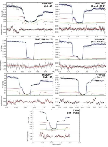
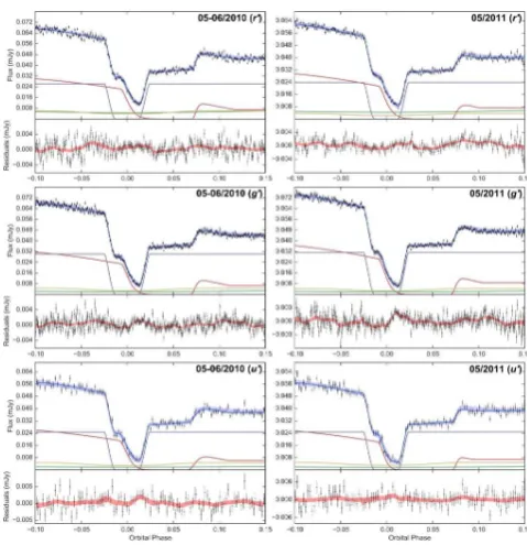
Posterior probability distributions of all parameters in the binary model were estimated using a Markov Chain Monte Carlo (MCMC) approach. The full results of all eclipse fits are shown in Figures A1–A15. Figure 1 shows an example g′-band eclipse light curve fit for each system.
In addition to the most probable fit of the eclipse model (blue line), a blue band is plotted that covers1σ from the mean of a random sample (size 1000) of the MCMC chain. The grey points represent the actual eclipse light curves, while the black points are the result of subtracting the GP’s posterior mean (itself shown,±1σ, by the red band covering the residuals below each plot). Also plotted are the sepa-rate components of the eclipse model: white dwarf (purple), bright spot (red), accretion disc (yellow) and donor (green).
4.2 System Parameters
Once the parameters of the binary model are estimated, the system parameters can be found. A full discussion can be found inMcAllister et al.(2017a). In brief, this involves an iterative procedure where the white dwarf spectral energy distribution (SED) – measured from the eclipse depth of the white dwarf – is fit by white dwarf atmosphere mod-els (Bergeron et al. 1995). This yields estimates of the white
D
o
w
n
lo
a
d
e
d
fro
m
h
ttp
s:
//a
ca
d
e
mi
c.
o
u
p
.co
m/
mn
ra
s/
a
d
va
n
ce
-a
rt
icl
e
-a
b
st
ra
ct
/d
o
i/1
0
.1
0
9
3
/mn
ra
s/
st
z9
7
6
/5
4
7
9
2
5
5
b
y
U
n
ive
rsi
ty
o
f S
h
e
ffi
e
ld
u
se
r
o
n
2
5
A
p
ri
l 2
0
1
Figure 1.Eclipse model fits tog-band light curves of 15 CVs. The lightcurves are shown in grey points; see Section4.1for full details of what is plotted. The system name is displayed in the top-right corner of each plot, along with whether the eclipse is an individual (Ind) or average (Ave) eclipse. For individual eclipses the cycle number is shown, while for average eclipses the month and year of the eclipses is shown. See AppendixAfor a complete set of eclipse plots.
dwarf temperatureT1 and distance d. The values ofq,∆Φ
and R1/a from the binary model, combined with Kepler’s
third law and a temperature-corrected mass-radius relation-ship for the white dwarf, are used to calculate the posterior probability distribution functions (PDFs) of the system pa-rameters:
• mass ratio,q;
• white dwarf mass,M1; • white dwarf radius,R1; • white dwarflogg; • donor mass,M2;
• donor radius, R2;
• binary separation, a;
• inclination,i.
System parameter values (see Table 2) were then ob-tained from the peak of each posterior PDF, with errors from the 67% confidence level. The results of the white dwarf SED fits are shown in Figure2, and the resultingT1anddvalues
for each system are also displayed in Table2. Note that the white dwarf flux fitting was not carried out for either IY UMa or SDSS 1006, due to the lack ofu′-band eclipses in
their eclipse model fits. Thankfully, precise measurements
D
o
w
n
lo
a
d
e
d
fro
m
h
ttp
s:
//a
ca
d
e
mi
c.
o
u
p
.co
m/
mn
ra
s/
a
d
va
n
ce
-a
rt
icl
e
-a
b
st
ra
ct
/d
o
i/1
0
.1
0
9
3
/mn
ra
s/
st
z9
7
6
/5
4
7
9
2
5
5
b
y
U
n
ive
rsi
ty
o
f S
h
e
ffi
e
ld
u
se
r
o
n
2
5
A
p
ri
l 2
0
1
Figure 1.Continued.
of T1 for both IY UMa1 (18000±1000 K) and SDSS 1006
(16000±1000 K) from spectral fitting are given inPala et al.
(2017).
As a sanity check on our white dwarf atmosphere fit-ting, we can compare the derived distances with the paral-laxes found in Gaia DR2 (Lindegren et al. 2018). We naively converted our distances to parallaxes, and compared to the parallaxes in Gaia DR2. The results are perfectly consistent with Gaussian statistics; the parallaxes of all but 4 out of
1 IY UMa entered outburst between the observations of
Pala et al. (2017) and this work, so this T1 measurement may
be slightly lower thanT1of the white dwarf in the eclipse light curves.
15 CVs agree within 1 standard deviation, whilst the most discrepant CV (GY Cnc) has a 2σdiscrepancy between our derived distance and the Gaia DR2 parallax. This gives us confidence on our distance estimates and also their uncer-tainties.
In section5we discuss the implications of the measured system parameters for CV evolution. However, before then, we discuss some remarkable aspects of the data for two in-dividual systems.
D
o
w
n
lo
a
d
e
d
fro
m
h
ttp
s:
//a
ca
d
e
mi
c.
o
u
p
.co
m/
mn
ra
s/
a
d
va
n
ce
-a
rt
icl
e
-a
b
st
ra
ct
/d
o
i/1
0
.1
0
9
3
/mn
ra
s/
st
z9
7
6
/5
4
7
9
2
5
5
b
y
U
n
ive
rsi
ty
o
f S
h
e
ffi
e
ld
u
se
r
o
n
2
5
A
p
ri
l 2
0
1
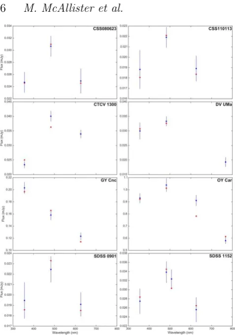
Figure 2. White dwarf fluxes for 13 CVs, showing the white dwarf fluxes from the eclipse model fits (blue) and white dwarf atmosphere predictions (red), at wavelengths corresponding tou′ (355.7 nm),g′(482.5 nm),KG5(507.5 nm),r′(626.1 nm) andi′ (767.2 nm) filters. The name of each system is displayed in the top-right corner of each plot.
[image:7.595.43.282.498.747.2]Figure 2.Continued.
Figure 3.O−Cdiagram for all 12 available ULTRACAM eclipses
of SDSS 1501, spanning∼8 yrs. The vertical dashed line corre-sponds to Sep 2010, when SDSS 1501 was reportedly observed in superoutburst. They-axis covers±15 s.
4.3 White Dwarf Flux and Orbital Period Variations in SDSS 1501
The eclipses of SDSS 1501 are white dwarf dominated, but some show faint bright spot features. There are a total of 15 available ULTRACAM eclipses of SDSS 1501, obtained during observing runs in 2004 (one eclipse), 2006 (eight), 2010 (two) and 2012 (one) (see Table C1 for further de-tails). However, only the single eclipses from 2004 and 2012 show signs of a bright spot eclipse, so both2were chosen for simultaneous eclipse modelling described above.
It became apparent that there was an appreciable in-crease in white dwarf flux across all three (u′
g′r′) bands
between the 2004 and 2012 eclipses. For this reason, model atmosphere fitting to the white dwarf fluxes was carried out separately for each eclipse, as shown in Figure 2. The re-sultingdandT1 for each eclipse are shown in Table2. The
white dwarf in 2012 appears marginally hotter, but note the 1.6σ discrepancy in d, which should of course remain constant. Both distances are formally consistent with a for-mal inference of the distance from Gaia DR2, including a weak distance prior (Bailer-Jones et al. 2018). However, the most likely distance from Gaia DR2 is 340 pc; favouring the 2012 distance estimate. The white dwarf flux fitting was re-peated for both eclipses, but this time with d held fixed at 360 pc. This now gives T1(2004) = 12100 ± 300 K and
T1(2012)=15800±300 K, a much larger increase of 3700 K.
Such a large discrepancy inT1 indicates that the white dwarf in SDSS 1501 underwent a period of enhanced ac-cretion between 2004 and 2012, most likely a superoutburst. According to vsnet-alert 121693, the superoutburst occurred in Sep 2010, with the observer claiming to have observed SDSS 1501 in outburst in addition to obtaining part of a superhump. Unfortunately, there is not enough coverage of this outburst to determine a superhump period.
2 Each ULTRACAM eclipse is in three bands (u′g′r′), giving six individual eclipses for modelling.
3
http://ooruri.kusastro.kyoto-u.ac.jp/mailarchive/vsnet-alert/12169
D
o
w
n
lo
a
d
e
d
fro
m
h
ttp
s:
//a
ca
d
e
mi
c.
o
u
p
.co
m/
mn
ra
s/
a
d
va
n
ce
-a
rt
icl
e
-a
b
st
ra
ct
/d
o
i/1
0
.1
0
9
3
/mn
ra
s/
st
z9
7
6
/5
4
7
9
2
5
5
b
y
U
n
ive
rsi
ty
o
f S
h
e
ffi
e
ld
u
se
r
o
n
2
5
A
p
ri
l 2
0
1
In addition to the white dwarf flux variations, SDSS 1501 also exhibits small orbital period variations. The white dwarf-dominated SDSS 1501 eclipses enable very pre-cise eclipse times to be obtained. We show the mid-eclipse times – after the subtraction of a linear ephemeris – in Figure3. The orbital period of SDSS 1501 appears to depart from linearity by approximately ±7 s over the∼8 yr ULTRACAM observational baseline. Such variations are not uncommon in CVs, and are thought to be caused by a magnetically-driven process within the donor. However, they are not observed in CVs with donors of spectral type later than M6 (Bours et al. 2016), due to magnetic activity in the donor decreasing with later spectral types. SDSS 1501’s donor mass obtained through eclipse modelling is substel-lar (0.061±0.004 M⊙), strongly indicating a spectral type
later than M6, and so the observation of period variations is surprising.
A logical deduction from looking at Figure3is that the superoutburst from Sep 2010 (dashed line) may have caused the observed change in orbital period, as the ephemeris ap-pears approximately linear up until this point. In this sce-nario, the 2012 eclipse occurs∼21 s later than expected, im-plying an increase in SDSS 1501’s orbital period of 0.0016 s (∆Porb/Porb=3.2×10−7). It is not clear how the
superout-burst could have caused such a large change in the orbital pe-riod. If some fraction of the disc mass was ejected during su-peroutburst, we would expect∆Porb/Porb=2Mej/(M1+M2),
whereMejis the mass ejected. This implies ejected masses of
10−7M
⊙, and disc masses in excess of this. A period change
might be induced by a change in the quadropole moment of the white dwarf and disc, due to the disc draining onto the white dwarf. In this case,Applegate(1992) gives
∆Porb/Porb≈ −
9∆Q
M1a2,
where ∆Q is the change in quadropole moment. We can obtain an order-of-magnitude estimate for∆Qif we ap-proximate the disc as a ring of mass Md and radius a/3,
and assume that during superoutburst the disc completely drains onto the white dwarf, giving ∆Q≈ −Mda2/9.
There-fore∆Porb/Porb≈Md/M1, again implying disc masses of or-der10−7M
⊙. With SDSS 1501’s system parameters known
(Table 2), the pre-outburst white dwarf temperature can be used to determine a medium-term average mass trans-fer rate for SDSS 1501 (Townsley & Bildsten 2003, 2004;
Townsley & G¨ansicke 2009) ofM˙ =9.3×10⁻¹¹M
⊙yr−1.
Pe-riod minimum systems are observed to have superoutburst cycles of order 20–30 yrs. Therefore the required disc masses are unrealistic, and the Sep 2010 superoutburst is not (at least not fully) responsible for the period variations exhib-ited by SDSS 1501. Another possible cause of the period variations is the presence of a third body within the system, however additional precise mid-eclipse timings are required in order to investigate this further.
4.4 Observed Low State of V713 Cep
The ULTRACAM/ULTRASPEC data archive contains a to-tal of 15 V713 Cep eclipses, with two ULTRACAM eclipses (cycle nos. 11 [u′
g′r′] and 3655 [u′g′i′]) showing clear
bright-spot features suitable for eclipse modelling. A feature of
Figure 4.g′-band eclipse light curve (24 Jun 2015, cycle no.
11955) of V713 Cep during a low state.
these two eclipses is a notable disc contribution (see Fig-ure A14), which is seen in all other V713 Cep eclipses in the archive, with the exception of one. The ULTRACAM
u′
g′r′eclipse of 24 Jun 2015 (cycle no. 11955,g′-band eclipse
shown in Figure4) contains no obvious signs of either a disc or bright spot eclipse, and at first glance resembles an eclipse of a detached, non-accreting binary. However, on closer in-spection there are signs of flickering outside of white dwarf eclipse, as well as a very slight curvature inside eclipse. These two features are both evidence for the presence of an – al-beit considerably diminished – accretion disc. A dwindling accretion disc and no sign of a bright spot indicates that the secondary has stopped supplying the disc with material and the system is in what is known as a ‘low state’.
Low states are relatively common phenomena for both magnetic CVs and a subgroup of novalike (NL) CVs called VY Scl stars, however they appear to be very rare (and un-expected) for DNe below the period gap. In fact, there is only one other documented occurrence in the literature – an extended (>2 yrs) low state of IR Com (Manser & G¨ansicke 2014). Given the rarity of low states in DNe, it is notable that IR Com and V713 Cep have similar orbital periods, just at the lower edge of the period gap. With only one eclipse of V713 Cep obtained during its low state, it is not known exactly how long this low state lasted. An upper limit of 403 days can be estimated based on the timings of other ULTRA-CAM eclipses, and therefore it was significantly shorter than the low state of IR Com.
5 DISCUSSION
With the new and revised system parameters obtained in this work, we now discuss what impact these results may have on the current understanding of CVs and their evolu-tion. In what follows, we combine the parameters presented here with a compilation of reliable parameters for 46 CVs from the literature. This compilation is presented in Ta-bleB1.
It has been shown that there is a significant discrep-ancy between the mean white dwarf mass in the field and that within CVs. Zorotovic et al. (2011) obtained a mean CV white dwarf mass of 0.82±0.03 M⊙, and an intrinsic
scatter of white dwarf masses of σ = 0.15 M⊙. With the
D
o
w
n
lo
a
d
e
d
fro
m
h
ttp
s:
//a
ca
d
e
mi
c.
o
u
p
.co
m/
mn
ra
s/
a
d
va
n
ce
-a
rt
icl
e
-a
b
st
ra
ct
/d
o
i/1
0
.1
0
9
3
/mn
ra
s/
st
z9
7
6
/5
4
7
9
2
5
5
b
y
U
n
ive
rsi
ty
o
f S
h
e
ffi
e
ld
u
se
r
o
n
2
5
A
p
ri
l 2
0
1
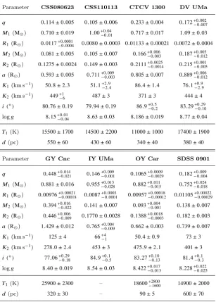
Parameter CSS080623 CSS110113 CTCV 1300 DV UMa
q 0.114±0.005 0.105±0.006 0.233±0.004 0.172+0.002
−0.007
M1(M⊙) 0.710±0.019 1.00+0.04
−0.01
0.717±0.017 1.09±0.03
R1(R⊙) 0.0117+0.0001
−0.0004
0.0080±0.0003 0.01133±0.00021 0.0072±0.0004
M2(M⊙) 0.081±0.005 0.105±0.007 0.166+0
.006
−0.003 0.187
+0.003
−0.012
R2(R⊙) 0.1275±0.0024 0.149±0.003 0.2111+0.0025
−0.0014
0.215+0.001
−0.005
a(R⊙) 0.593±0.005 0.711+0.009
−0.003 0.805
±0.007 0.889+0.006
−0.012
K1(km s−1) 50.8±2.3 51.1+2.9
−2.4
86.4±1.4 76.1+0.9
−2.9
K2(km s−1) 449+−16 487±3 371±3 444±4
i(◦) 80.76±0.19 79.94±0.19 86.9+0.5
−0.2 83.29
+0.29
−0.10
logg 8.15+0.01
−0.04
8.63±0.03 8.186±0.019 8.77±0.04
T1(K) 15500±1700 14500±2200 11000±1000 17400±1900
d(pc) 550±60 430±60 340±40 380±40
Parameter GY Cnc IY UMa OY Car SDSS 0901
q 0.448+0.014
−0.021
0.146+0.009
−0.001
0.1065+0.0009
−0.0029
0.182+0.009
−0.004
M1(M⊙) 0.881±0.016 0.955+0.013
−0.028 0.882
+0.011
−0.015 0.752
+0.024
−0.018
R1(R⊙) 0.00976+0
.00021
−0.00018 0.0087
+0.0003
−0.0001 0.00957
+0.00018
−0.00012 0.01105 +0.00022 −0.00029
M2(M⊙) 0.394+0.016
−0.022
0.141±0.007 0.093+0.004
−0.001
0.138±0.007
R2(R⊙) 0.446+0.006
−0.009 0.1770
±0.0028 0.1388+0.0018
−0.0003 0.182
±0.003
a(R⊙) 1.429±0.012 0.765+0.004
−0.009
0.662±0.003 0.739±0.007
K1(km s−1) 125±4 66+4
−1 50.4±0.9 73±3
K2(km s−1) 278.0±2.4 453±3 475.9±2.1 401±3
i(◦) 77.06+0.29
−0.18 84.9
+0.1
−0.5 83.27
+0.10
−0.13 81.4
+0.1
−0.3
logg 8.40±0.019 8.54±0.03 8.422+0.017
−0.013 8.228
+0.022
−0.025
T1(K) 25900±2300 – 18600+2800
−1600 14900±2000
[image:9.595.140.448.105.535.2]d(pc) 320±30 – 90±5 600±70
Table 2.System parameters for the 15 eclipsing systems analysed in this paper.
updated sample of CV masses now available, we can revise the mean white dwarf mass in CVs, following the procedure outlined in Appendix B ofKnigge(2006), to0.81±0.02 M⊙
(σ = 0.13 M⊙), entirely consistent with Zorotovic et al’s
value.
One way to explain the presence of high white dwarf masses in CVs is through white dwarf mass growth through steady accretion across the lifetime of a CV. Since CVs evolve to shorter orbital periods over their lives, this requires the observation of higher white dwarf masses in systems with lower orbital periods. To test this, hM1i was re-calculated
for 31 systems below the period gap (Porb ∼ 2.15 hrs),
giving hM1i(below gap) = 0.81±0.02 M⊙ (σ = 0.10 M⊙),
and for 16 systems above the gap (Porb ∼ 3.18 hrs), giving
hM1i(below gap) =0.82±0.02 M⊙ (σ =0.10 M⊙). We
there-fore see no evidence for white dwarf mass growth in CVs. While white dwarf mass growth in CVs appears doubtful,
further precise white dwarf masses from systems at long pe-riod (>3 hrs) are required before it can be entirely dismissed.
5.1 Testing the Validity of the Empirical CAML Model
An alternative explanation for the high white dwarf mass in CVs was proposed by Schreiber et al. (2016). The authors put forward an empirical consequential angular momentum loss (eCAML) model, which produces a dynamical stabil-ity limit onq, causing systems with low-mass white dwarfs to become unstable to mass transfer. These systems con-sequently merge, removing them from the CV population. The eCAML model is attractive as it can simultaneously ex-plain the low observed space density of CVs (Belloni et al. 2018) and the origin of isolated low-mass white dwarfs
(Zorotovic & Schreiber 2017).
The top-left plot of Figure 2 inSchreiber et al. (2016)
D
o
w
n
lo
a
d
e
d
fro
m
h
ttp
s:
//a
ca
d
e
mi
c.
o
u
p
.co
m/
mn
ra
s/
a
d
va
n
ce
-a
rt
icl
e
-a
b
st
ra
ct
/d
o
i/1
0
.1
0
9
3
/mn
ra
s/
st
z9
7
6
/5
4
7
9
2
5
5
b
y
U
n
ive
rsi
ty
o
f S
h
e
ffi
e
ld
u
se
r
o
n
2
5
A
p
ri
l 2
0
1
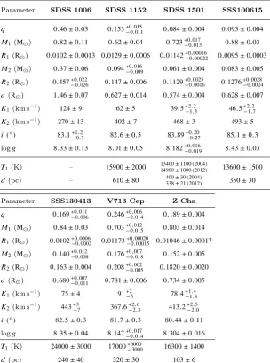
Parameter SDSS 1006 SDSS 1152 SDSS 1501 SSS100615
q 0.46±0.03 0.153+0.015
−0.011 0.084
±0.004 0.095±0.004
M1(M⊙) 0.82±0.11 0.62±0.04 0.723+0.017
−0.013
0.88±0.03
R1(R⊙) 0.0102±0.0013 0.0129±0.0006 0.01142+0.00016
−0.00022
0.0095±0.0003
M2(M⊙) 0.37±0.06 0.094+0
.016
−0.009 0.061
±0.004 0.083±0.005
R2(R⊙) 0.457+0.022
−0.026
0.147±0.006 0.1129+0.0025
−0.0016
0.1276+0.0028
−0.0024
a(R⊙) 1.46±0.07 0.627±0.014 0.574±0.004 0.628±0.007
K1(km s−1) 124±9 62±5 39.5+2.2
−1.3
46.5+2.2
−1.7
K2(km s−1) 270±13 402±7 468±3 493±5
i(◦) 83.1+1.2
−0.7 82.6
±0.5 83.89+0.20
−0.27 85.1
±0.3
logg 8.33±0.13 8.01±0.05 8.182+0.016
−0.019
8.43±0.03
T1(K) – 15900±2000 13400±1100 (2004)
14900±1000 (2012) 13600±1500
d(pc) – 610±80 400±30 (2004)
338±21 (2012) 350±30
Parameter SSS130413 V713 Cep Z Cha
q 0.169+0.011
−0.006
0.246+0.006
−0.014
0.189±0.004
M1(M⊙) 0.84±0.03 0.703+0
.012
−0.015 0.803
±0.014
R1(R⊙) 0.0102+0.0006
−0.0002
0.01173+0.00020
−0.00015
0.01046±0.00017
M2(M⊙) 0.140+0.012
−0.008 0.176
+0.007
−0.018 0.152
±0.005
R2(R⊙) 0.163±0.004 0.208+0.002
−0.005
0.1820±0.0020
a(R⊙) 0.680+0.007
−0.011 0.781
±0.006 0.734±0.005
K1(km s−1) 75±4 91+2
−5 78.4+
1.4
−1.8
K2(km s−1) 443+−37 367.6+ 2.6
−2.3
413.2+2.5
−2.0
i(◦) 82.5±0.3 81.7±0.3 80.44±0.11
logg 8.35±0.04 8.147+0.017
−0.014
8.304±0.016
T1(K) 24000±3000 17000+6000
−3000 16300±1400
[image:10.595.142.447.104.514.2]d(pc) 240±40 320±30 103±6
Table 2.Continued.
was updated to take into account the results of this work (Figure 5). This plot is in M2 vs q parameter space, with
regions (grey) that are theoretically prohibited due to con-straints put on M1. The dark grey prohibited region in the
bottom right of Figure5is an upper mass limit on M1,
re-sulting from the Chandrasekhar mass limit of a white dwarf (1.44 M⊙). The light grey prohibited region is a lower mass
limit on M1and is a consequence of the dynamical stability limit onq supplied by the eCAML model. Also plotted in Figure5are systems with measured M2 andq, either from this work (green points) or elsewhere (black/blue points; see TableB1). These systems with measured system parameters provide a test of the eCAML model, as all should lie within the valid region (white). Any systems lying inside the pro-hibited dynamically unstable region would compromise the credibility of the model.
All systems modelled in this work lie comfortably within the valid region of Figure 5, along with the vast major-ity of other systems. Two appear to (just) violate the dynamical instability constraint, namely SDSS 0756+0858
(Tovmassian et al. 2014) and DQ Her (Horne et al. 1993),
however both systems could feasibly be stable under the eCAML model after taking into account their uncertainties. This outcome offers support to the validity of the eCAML model as a solution to the CV white dwarf mass problem, however a much larger sample of systems with precise system parameters is necessary in order to provide a more stringent test of the model.
5.2 Reviewing the Properties of the Period Spike
The period spike is a feature of the orbital period distribu-tion which is expected to occur as systems “pile-up” near the orbital period minimum due to the long evolutionary timescale. It was finally observed byG¨ansicke et al.(2009) through analysing the orbital period distribution of newly identified CVs from SDSS (York et al. 2000). These systems were all identified spectroscopically (e.g.Szkody et al. 2002), and therefore not affected by the same biases/limitations as systems discovered through other means, e.g. DN outbursts
D
o
w
n
lo
a
d
e
d
fro
m
h
ttp
s:
//a
ca
d
e
mi
c.
o
u
p
.co
m/
mn
ra
s/
a
d
va
n
ce
-a
rt
icl
e
-a
b
st
ra
ct
/d
o
i/1
0
.1
0
9
3
/mn
ra
s/
st
z9
7
6
/5
4
7
9
2
5
5
b
y
U
n
ive
rsi
ty
o
f S
h
e
ffi
e
ld
u
se
r
o
n
2
5
A
p
ri
l 2
0
1
M1 > 1.44 M
Dynamically Unstable
M1 < 0.15 M
Figure 5. q vs M2 plot for CVs. The grey regions are
theoretically prohibited due to constraints put on M1. The dark grey regions cover unrealistically low white dwarf masses (.0.15 M⊙) and masses greater than the Chandrasekhar mass limit (1.44 M⊙), while the light grey region is forbidden by the empirical consequential angular momentum loss (eCAML) model
of Schreiber et al. (2016). The dashed grey line represents the
mean value of M1 from this work. The green and black points represent masses obtained from eclipse modelling of ULTRA-CAM/ULTRASPEC data, either from this work (green) or other-wise (black). The faint blue points represent measured CV masses from other methods: eclipse modelling of other data (circles), con-tact phase timing (squares), and radial velocity (triangles).
and X-ray emission (see G¨ansicke et al. 2009 for more de-tails). Spectroscopic identification, coupled with a survey depth of g′ ∼19.5, gives this particular sample the ability
to provide the closest representation of the true orbital pe-riod distribution of CVs to date, a claim supported by the emergence of the long predicted-but-elusive period spike at the period minimum. G¨ansicke et al.(2009) produced esti-mates for the location (82.4±0.7 min) and width (FWHM = 5.7 min) of the period spike. Eight years on, the sam-ple has increased and morePorbmeasurements have become available, enabling the orbital period distribution – and in particular the properties of the period spike – to be reviewed.
TheG¨ansicke et al.(2009) sample consisted of 49
spec-troscopically identified SDSS CVs below the period gap
(Porb . 129min; Knigge 2006) with precise Porb
measure-ments (errors<30s). Precise Porbmeasurements for an
ad-ditional 23 systems (and updated measurements for a hand-ful from the original sample) have since become available, increasing the sample to 72 systems. Of the new systems, six are eclipsing systems with observations using ULTRA-CAM/ULTRASPEC, 10 are fromThorstensen et al.(2015,
2017) and the remaining seven are from theRitter & Kolb
(2003) catalogue (v7.24; see references within). All systems were discovered by the SDSS (e.g. Szkody et al. 2011) ex-cept two, PHL 1445 and CSS110113, which were discovered by the 6dF Galaxy Survey (6dFGS;Jones et al. 2004).
Figure 6 shows the orbital period distribution of all 72 spectroscopically identified CVs in the form of both a histogram (red) and cumulative plot (blue). As with the
G¨ansicke et al. (2009) sample (dark red histogram), the
new sample shows a clear accumulation of systems cen-tred around ∼82 min, which is clearly identifiable as the period spike. Estimating Pspike involved the fitting of a
Figure 6. Histogram (red) and cumulative plot (blue) for 72
spectroscopically identified (from SDSS and 6dFGS) CVs below the period gap with precisePorb measurements (sub-30 s errors). For comparison, the sample ofG¨ansicke et al.(2009) is also shown (dark red histogram), in addition to the position and FWHM of the period spike estimated in the same study (black bar).
Gaussian distribution to the orbital period distribution be-tween 77 and 87 min. An estimate ofPspike=82.7±0.4min (σ = 2.35min, FWHM =5.53min) was obtained, which is largely unchanged from theG¨ansicke et al. (2009) sample. This is not surprising, as the majority (∼75%) of additional systems havePorb> 89min, and therefore do not belong to the period spike.
We note here that there is a hint of bi-modality in the period distribution of systemsbelowthe period gap, with a dearth of systems with orbital periods around 88 minutes. A Hartigan dip test (Hartigan & Hartigan 1985) reveals that this is not statistically significant.
5.3 Updating the Calibration of the superhump period excess-mass ratio Relation
During superoutburst the accretion disc is driven into an elliptical state by resonances between the donor star and material within the disc. Tidal interactions between the el-liptical disc and the donor lead to periodic fluctuations in the elliptical, precessing, disc known as superhumps. The disc precesses at a slow rate, with a period (Pprec)
signifi-cantly longer than Porb. These two periods therefore both
contribute to the formation of the superhump period (Psh), which is simply the ‘beat period’ ofPprec and Porb(Hellier
2001):
1
Psh =
1
Porb−
1
Pprec
. (1)
Pshis therefore usually a few percent longer than Porb, but does not stay constant throughout the superoutburst. In fact, a superoutburst can be split up into three distinct stages (A, B and C), with sharp transitions observed be-tween each stage. Stage A represents the start of the super-outburst, with a long, stablePsh. Stage B is the middle part
of the superoutburst, with a shorter, unstablePsh. The final
stage (C) exhibits the shortestPsh, which is stable once again
(Olech et al. 2003;Kato et al. 2009). The general trend of
decreasingPshacross the superoutburst hints at an
increas-D
o
w
n
lo
a
d
e
d
fro
m
h
ttp
s:
//a
ca
d
e
mi
c.
o
u
p
.co
m/
mn
ra
s/
a
d
va
n
ce
-a
rt
icl
e
-a
b
st
ra
ct
/d
o
i/1
0
.1
0
9
3
/mn
ra
s/
st
z9
7
6
/5
4
7
9
2
5
5
b
y
U
n
ive
rsi
ty
o
f S
h
e
ffi
e
ld
u
se
r
o
n
2
5
A
p
ri
l 2
0
1
ing Pprec (from equation 1) and therefore a dwindling disc radius (Murray 2000).
The superhump excess (ǫ) is defined asǫ= Psh−Porb Porb , and is directly related to the mass ratio,q. A calibration of this relationship (e.gPatterson et al. 2005;Knigge 2006) allows estimates of mass ratios for all superhumping systems. From this current work and the work of others (e.g.Savoury et al. 2011), new potential calibration systems have emerged, in addition to revisedqvalues for existing calibration systems. Revised superhump periods have also been measured, cour-tesy of the SU UMa-type DNe survey of Kato et al.(2009,
2010, 2012, 2013, 2014a,b, 2015, 2016, 2017). With all of
these new measurements becoming available since the work
ofKnigge(2006), it is appropriate to update the calibration
of theǫ(q) relation.
Table3contains all of the calibrating systems currently available4, along with their orbital and superhump periods (and references). The two superhump period columns, PshB
and PC
sh, represent the superhump periods during stage B
and stage C of superoutburst, respectively. All but the final four systems in Table3are SU UMa-type DNe that undergo superoutbursts. The other four systems are either Classical Novae or Novalikes that display permanent superhumps, and it is assumed these superhump periods resemble those ofPB
sh
for SU UMa-type DNe.
For each system in Table3, the superhump period ex-cess was calculated for stage B (ǫB) and stage C (ǫC)
de-pending on PshB/PC
sh availability. Figure 7 shows ǫB plotted
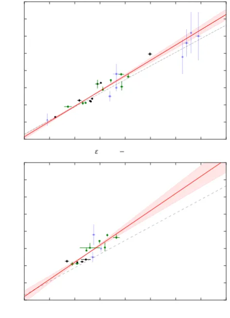
against qfor the 24 calibration systems from Table3with availablePBshmeasurements. The dashed grey line shows the existing calibration from Knigge(2006), while the red line represents the following, updated linear calibration:
q(ǫB)=(0.118±0.003)+(4.45±0.28)×(ǫB−0.025). (2)
This updated calibration was obtained through the same
χ2 minimisation technique employed byKnigge(2006) (see Appendix A of reference), and has an intrinsic dispersion (σ) of 0.012. While there is good coverage for systems with
0.1<q<0.2, more calibration systems withqoutside this range are required in order to further constrain the gradi-ent. For example, due to its position in Figure7, SDSS 1702 (q≈0.25) has a rather large influence on the gradient, so therefore more systems with precisely measured values of
q greater than 0.2 are highly coveted. Unfortunately, this includes period gap systems, which are rare, and systems above the gap, for which precise measurements ofqare hard to obtain. It is clear from Figure7that the new calibration has a steeper gradient that the existing one from Knigge
(2006). A possible reason for this is the variation in measure-ment ofPshbetweenPatterson et al.(2005) andKato et al.
(2009); the sources ofPshfor both the existing and new
cal-ibration, respectively.Patterson et al. (2005) measures Psh
from ‘common’ superhumps, which typically cover stage B, but can also cover only a fraction of this stage or spread into stages A and C.
The same treatment was given to the 15 calibration sys-tems in Table3with availablePC
shmeasurements, producing
4 The calibration system KV UMa used byKnigge(2006) was not included on the basis of it being a low-mass X-ray binary, rather than a CV.
0.00 0.01 0.02 0.03 0.04 0.05 0.06 0.07 0.08
= (Psh Porb)/Porb
0.00 0.05 0.10 0.15 0.20 0.25 0.30 0.35 0.40
q
=
M2 /M1
0.00 0.01 0.02 0.03 0.04 0.05 0.06 0.07 0.08 ǫ =(Psh−Porb)/Porb
0.00 0.05 0.10 0.15 0.20 0.25 0.30 0.35 0.40
q
=
M2
/M
1
Figure 7.MeasuredǫBandqvalues of superhumping and
eclips-ing CVs, with the same data point colour/shape scheme as Fig-ure5. The dashed grey line shows the existing linear calibration of theǫ(q) relation for superhumping CVs fromKnigge(2006), while the red line shows an updated calibration from this work. The red shaded region represents 1σerrors. The top plot shows the relationship for stage B superhumps, the bottom plot that for stage C superhumps.
the following linear relation (withσ=0.012again inferred):
q(ǫC)=(0.135±0.004)+(5.0±0.7)×(ǫC−0.025). (3)
This relation is also shown in Figure7.
5.4 Donor Masses and Radii of Superhumping CVs
Given our updating of the superhump-mass ratio relations above, we revisit the analysis of donor star properties in
Knigge(2006) and Knigge et al. (2011). Firstly,Psh values
for all SU UMa-type DNe in thePatterson et al.(2005) sam-ple (70 systems) were replaced by PB
sh measurements from
the SU UMa-type DNe survey of Kato et al. (2009, 2010,
2012, 2013, 2014a,b, 2015, 2016, 2017). For a number of
systems, Porb was also updated, either from measurements
made by Kato et al., or additional studies (see references within Kato et al.). Values of ǫB were obtained from PshB
andPorb, then subsequently converted intoqvia the newly
calibratedǫB(q) relation (equation2). Equation2was also
used to determineqfor the eight systems displaying perma-nent superhumps. Assuming a constant white dwarf mass of
D
o
w
n
lo
a
d
e
d
fro
m
h
ttp
s:
//a
ca
d
e
mi
c.
o
u
p
.co
m/
mn
ra
s/
a
d
va
n
ce
-a
rt
icl
e
-a
b
st
ra
ct
/d
o
i/1
0
.1
0
9
3
/mn
ra
s/
st
z9
7
6
/5
4
7
9
2
5
5
b
y
U
n
ive
rsi
ty
o
f S
h
e
ffi
e
ld
u
se
r
o
n
2
5
A
p
ri
l 2
0
1
[image:12.595.304.541.104.431.2]System Porb(d) PBsh(d) P C
sh(d) Ref.(s)
SDSS 1507 0.04625828(4) 0.046825(4) – 1,2 SSS100615∗ 0.0587045(4)§ 0.05972(9) – 3 SDSS 1502 0.05890961(5) 0.060463(13) 0.060145(19) 1,4 SDSS 0903 0.059073543(9) 0.06036(5) 0.06007(5) 1,4 ASASSN-14ag 0.060310665(9)§ 0.06206(6) – 5 XZ Eri 0.061159491(5) 0.062807(18) 0.06265(12) 1,6 SDSS 1227 0.062959041(7) 0.064604(29) 0.06440(5) 1,7 OY Car∗ 0.06312092545(24)§ 0.064653(28) 0.06444(5) 8 SSS130413∗ 0.0657692903(12)§ – 0.06751(24) 5 CSS110113∗ 0.0660508707(18)§ 0.067583(26) 0.06731(4) 7 SDSS 1152∗ 0.0677497026(3)§ 0.07036(4) 0.069914(19) 8 OU Vir 0.072706113(5) 0.074912(17) – 1,6 IY UMa∗ 0.07390892818(21)§ 0.076210(25) 0.075729(19) 4 Z Cha∗ 0.0744992631(3)§ 0.07736(8) 0.076948(23) 5 SDSS 0901∗ 0.0778805321(5)§ 0.08109(5) 0.08072(10) 9 DV UMa∗ 0.0858526308(7)§ 0.08880(3) 0.08841(3) 6 SDSS 1702 0.10008209(9) 0.10507(8) – 1,6
WZ Sge 0.0566878460(3) 0.057204(5) – 6,10 V2051 Oph 0.06242785751(8)§ 0.06471(9) 0.06414(4) 5,11 HT Cas 0.0736471745(5)§ 0.076333(5) 0.075886(5) 3,12 V4140 Sgr 0.0614296779(9) 0.06351(4) 0.06309(7) 6,11
[image:13.595.151.437.105.394.2]V348 Pup 0.101838931(14) 0.108567(2)† – 13 V603 Aql 0.13820103(8) 0.14686(7)† – 14,15 DW UMa 0.136606499(3) 0.14539(13)† – 16,17 UU Aqr 0.1638049430 0.17510(18)† – 18,19
Table 3.Orbital (Porb) and superhump (Psh) periods of the systems used to calibrate theǫ(q)relation. The majority of systems are SU
UMa-type DNe, however the bottom four are CNe/NLs.PBshand PCshare the periods for stage B and C superhumps, respectively. See Tables2and B1forq values. References: (1)Savoury et al.(2011), (2)Patterson et al.(2017), (3)Kato et al.(2016), (4)Kato et al. (2010), (5) Kato et al. (2015), (6) Kato et al. (2009), (7) Kato et al. (2012), (8) Kato et al. (2017), (9) Kato et al. (2013), (10)
Patterson (1998), (11) Baptista et al. (2003), (12) Horne et al. (1991), (13) Rolfe et al. (2000), (14) Peters & Thorstensen (2006),
(15)Patterson et al. (1997), (16)Araujo-Betancor et al.(2003), (17)Patterson et al.(2002), (18) Baptista & Bortoletto(2008), (19)
Patterson et al.(2005).
∗Updatedqvalue produced in this work (Table2),†Superhump period from permanent superhumps,§P
orbfrom this work
hM1i=0.81 M⊙, donor mass estimates were obtained for all
systems in the superhumper sample.
As the donor fills its Roche lobe, theEggleton(1983) ap-proximation for the volume-averaged Roche lobe size, com-bined with Kepler’s 3rd law, can be used to obtain estimates for donor radii fromq,M2and Porb:
R2
R⊙ =
0.2478 M2
M⊙
!1/3
P2/3
orb
"
q1/3(1+q)1/3
0.6q2/3+ln(1+q1/3)
#
, (4)
where Porbis in units of hrs. TheEggleton (1983)
approxi-mation for the volume-averaged Roche lobe size is the same one used to determineR2for systems that have been eclipse
modelled, establishing consistency between the superhump-ing and eclipssuperhump-ing samples. It is important to note that
Knigge et al.(2011) use a more complex, accurate
approxi-mation for the volume-averaged size of the Roche lobe based on the results of Sirotkin & Kim (2009), which represents the donor as a polytrope, rather than a point source. How-ever, the advantage of using theSirotkin & Kim(2009) ap-proximation is small, with only a ∼1% difference between the two approximations (Figure 3 ofKnigge et al. 2011).
In addition to the 78 superhumper sample from
Patterson et al. (2005), Kato et al. provide PshB,C and Porb
values for a further 147 systems. These systems were given
the same treatment as the Patterson et al. (2005) sample (outlined above). A handful of systems only have available
PshCvalues, in which case equation3was used. This brings the total number of superhumping systems with inferred donor properties to 225.
5.5 Updating the Semi-Empirical Mass-Radius Relation for CV Donor Stars
With donor masses and radii for 15 eclipsing systems in this work, a further 31 (mostly) eclipsing systems from the lit-erature (see TableB1) and 225 superhumpers, it is possible to update the mass-radius relation for CV donor stars from
Knigge (2006) and Knigge et al. (2011). The same fitting
procedure used byKnigge(2006) was followed to update the mass-radius relation. Assumptions for some parameters in this model are required, since they are not well-constrained by the donor masses and radii. Assumptions for the donor mass within the period gap (Mconv), and the upper and lower (Pgap,+,Pgap,−) bounds of the period gap fromKnigge et al.
(2011) remained unchanged. We do adopt a smaller value
for Pbounce (called Pmin in Knigge et al. (2011)). Pbounce is
the orbital period where the pre-bounce and post-bounce
D
o
w
n
lo
a
d
e
d
fro
m
h
ttp
s:
//a
ca
d
e
mi
c.
o
u
p
.co
m/
mn
ra
s/
a
d
va
n
ce
-a
rt
icl
e
-a
b
st
ra
ct
/d
o
i/1
0
.1
0
9
3
/mn
ra
s/
st
z9
7
6
/5
4
7
9
2
5
5
b
y
U
n
ive
rsi
ty
o
f S
h
e
ffi
e
ld
u
se
r
o
n
2
5
A
p
ri
l 2
0
1
power-law relationships intersect.Knigge et al. (2011) used the location of the period spike fromG¨ansicke et al.(2009)
forPbounce. However, real systems do not reach this orbital
period, because the smooth track followed by real systems near period minimum is not well represented by two power laws. PHL 1445 (McAllister et al. 2015) is expected to be close to the absolute minimum period for main sequence CVs, and so its orbital period of 76.3 min is used forPbounce
here. The value ofMbounceshown above was determined from
the optimal short-period fit.
Mbounce=0.063+0.005
−0.002M⊙, Pbounce=76.3±1.0 min
Mconv=0.20±0.02 M⊙, Pgap,− =2.15±0.03 hrs,
Mevol≃0.6−0.8 M⊙, Pgap,+=3.18±0.04 hrs.
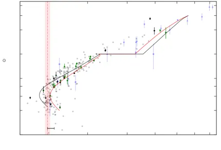
The donor masses and radii for all but 12 systems were included in the fits. The majority of these systems were ex-cluded due to being period gap systems (see grey box in bottom plot of Figure8), while SDSS 1507 (outlying black data point in period bouncer regime) was excluded as it is known to be a Galactic halo object (Patterson et al. 2008;
Uthas et al. 2011). The results from the three power law fits
are shown in Figure8, and take the following form:
R2
R⊙ =
0.109±0.003 M2
Mbounce
0.152±0.018
M2<Mbounce
0.225±0.008 M2
Mconv
0.636±0.012
Mbounce<M2 <Mconv
0.293±0.010 M2
Mconv
0.69±0.05
Mconv<M2<Mevol.
Comparing these results with Knigge et al. (2011), there is little change in the exponents of the mass-radius rela-tion in both the long- and short-period regimes. One no-table difference, however, is the amount of intrinsic scat-ter, σint, required for the short-period systems, reduced from approximately 0.02 R⊙ to 0.005 R⊙. The small
scat-ter provides strong evidence for a very tight evolutionary path followed by non-evolved CV donors, implying little spread in AML loss rates for CVs with the same compo-nent masses. The scatter within the long-period regime, at
0.04 R⊙, is almost a factor of 10 larger than that at short
periods. Figure 8 shows two outlying long-period systems
withR2≃0.40 R⊙, namely IP Peg (Copperwheat et al. 2010)
and HS 0220+0603 (Rodr´ıguez-Gil et al. 2015). The donors within these two systems are undersized for their masses, and may even be in thermal equilibrium, which is unex-pected for a CV donor. It is possible that both IP Peg and HS 0220+0603 have donors in thermal equilibrium due to recently starting mass transfer.
The mass-radius relation for period-bouncers has changed significantly. The new power law exponent of0.152±
0.018 is much smaller than that of Knigge et al. (2011),
a consequence of using lower values for both Mbounce and
Pbounce, in addition to the inclusion of many more
period-bouncers in the new donor sample, which enables a bet-ter constraint of the power law in this regime. There has been a long-standing issue with the number of confirmed period-bounce CVs, which has always been much lower than the predicted 40–70% (Goliasch & Nelson 2015;Kolb 1993). Whilst the sample of donor masses collected here is far from homogeneous, and the presence of large numbers of super-humping systems introduces complicated selection effects,
we note here that 30% of our sample has a donor mass be-low 0.063M⊙and are therefore likely to be period-bouncers.
5.6 Comparison to theoretical CV evolution tracks
In addition to a broken-power-law mass-radius relation for CV donors,Knigge et al. (2011) present a theoretical evo-lutionary track, produced with the aim of quantifying the secular mass transfer rate in CVs. The track which best reproduces their donor sample requires reduced magnetic braking above the gap (fMB =0.66±0.05), but additional angular momentum loss below the gap (fGR=2.47±0.22). The donor sample presented in this work is shown in the
M2-R2 and Porb-M2 planes in Figures 9 and 10,
respec-tively. Also shown is the ‘best fit’ track fromKnigge et al.
(2011), and the ‘standard’ track (fGR = fMB = 1). It is clear from these figures that the best-fit evolutionary track
fromKnigge et al. (2011) under predicts the donor mass at
orbital periods below the period gap, and has a period min-imum that is longer than that observed. This again implies that less additional angular momentum loss is needed below the period gap than suggested byKnigge et al. (2011). In contrast, we find that the ‘standard’ track provides a better fit to the donor sample immediately below the gap, where the donor mass is in the range 0.10–0.20 M⊙. This is most
apparent in Figure10. Although the standard track is a good fit to systems immediately below the gap, it diverges from the donor sequence at lower masses, and predicts a period minimum shorter than the observed value. Therefore, the donor properties in CVs appears to argue for an additional source of AML that is small compared to gravitational radia-tion just below the period gap, but becomes more significant at shorter orbital periods and/or donor masses.
The eCAML model ofSchreiber et al.(2016) might pro-vide something similar to the behaviour required. All models of CV evolution require a termν, which expresses the AML which arises as a consequence of mass transfer. In the stan-dard model, it is assumed that the mass lost from the white dwarf during nova eruptions carries with it the specific angu-lar momentum of the white dwarf, leading toν=M22/(M1M),
where M is the total mass of the system. In the eCAML model, an alternative form of ν∼0.35/M1 is proposed. We
used equation 1 fromKnigge et al. (2011) to roughly esti-mate the mass loss rates under the eCAML model at key points in the evolution of the donor. Just below the period gap, we takeM1=0.82M⊙,M2=0.15M⊙and we assume the
donor is roughly in thermal equilibrium, so the mass-radius index is ξ = 0.8. This implies that in the eCAML model, mass loss rates just after the period gap are only around 35% higher than the ‘standard’,fGR=1, model. For systems near
the period minimum, we takeM1=0.82M⊙,M2=0.065M⊙
andξ=−1/3, which suggests mass loss rates around 9 times higher than the fGR=1case. Therefore, the eCAML model provides a mass loss law which is qualitatively similar to the one implied by CV donor properties. However, it is worth bearing in mind that the ν ∼ 0.35/M1 prescription
is not physically motivated.Schreiber et al. (2016) suggest that angular momentum loss during nova outbursts might produce a similar behaviour, but the frequency of nova out-bursts will drop as the accretion rate falls. Therefore eCAML may be less important for CVs near the period minimum
D
o
w
n
lo
a
d
e
d
fro
m
h
ttp
s:
//a
ca
d
e
mi
c.
o
u
p
.co
m/
mn
ra
s/
a
d
va
n
ce
-a
rt
icl
e
-a
b
st
ra
ct
/d
o
i/1
0
.1
0
9
3
/mn
ra
s/
st
z9
7
6
/5
4
7
9
2
5
5
b
y
U
n
ive
rsi
ty
o
f S
h
e
ffi
e
ld
u
se
r
o
n
2
5
A
p
ri
l 2
0
1