Time varying dimension models

S

TRATHCLYDE

D

ISCUSSION

P

APERS IN

E

CONOMICS

D

EPARTMENT OF

E

CONOMICS

U

NIVERSITY OF

S

TRATHCLYDE

G

LASGOW

TIME VARYING DIMENSION MODELS

B

Y

JOSHUA

C.C.

CHAN,

GARY

KOOP,

ROBERT

LEON-GONZALEZ

AND

RODNEY

W.

STRACHAN

Time Varying Dimension Models

Joshua C.C. Chan

Australian National University

Gary Koop

University of Strathclyde

Roberto Leon-Gonzalez

National Graduate Institute for Policy Studies

Rodney W. Strachan

Australian National University

May 11, 2010

Abstract: Time varying parameter (TVP) models have enjoyed an in-creasing popularity in empirical macroeconomics. However, TVP models are parameter-rich and risk over-…tting unless the dimension of the model is small. Motivated by this worry, this paper proposes several Time Varying dimension (TVD) models where the dimension of the model can change over time, allowing for the model to automatically choose a more parsimonious TVP representation, or to switch between di¤erent parsimonious representa-tions. Our TVD models all fall in the category of dynamic mixture models. We discuss the properties of these models and present methods for Bayesian inference. An application involving US in‡ation forecasting illustrates and compares the di¤erent TVD models. We …nd our TVD approaches exhibit better forecasting performance than several standard benchmarks and shrink towards parsimonious speci…cations.

1

Introduction

It is common for researchers to model variation in coe¢ cients in time series models using state space methods. If, for t = 1; ::; T, yt is an n 1vector of observations on the dependent variables,Ztis ann mmatrix of observations on explanatory variables and tis anm 1vector of states, then such a state space model can be written as:

yt = Zt t+"t (1)

t+1 = t+ t;

where "t is N(0; Ht) and t is N(0; Qt). The errors, "t and t, are assumed to be independent (at all leads and lags and of each other). This framework can used to estimate time-varying parameter (TVP) regression models, vari-ants of which are commonly-used in macroeconomics (e.g., Groen, Paap and Ravazzolo, 2009, Koop and Korobilis, 2009). Furthermore, TVP-VARs (see among many others, Canova, 1993, Cogley and Sargent, 2005, D’Agostino, Gambetti and Giannone, 2009 and Primiceri, 2005) are obtained by lettingZt contain deterministic terms and appropriate lags of the dependent variables, setting Qt=Q and givingHt a multivariate stochastic volatility form.

a time-varying dimension (TVD) model where restrictions which reduce the dimension of the model are imposed only at some points in time.

There are also many econometrically-inspired reasons for being interested in TVD models. For instance, if lag length changes over time, then impos-ing di¤erent lag lengths at di¤erent points in time will lead to more precise estimates. In forecasting, the importance of shrinkage has been found in a myriad of studies (e.g. Groen, Paap and Ravazzolo, 2009 or Koop and Koro-bilis, 2009). In general, TVP models risk being over-parameterized. Allowing for the dimension of the model to change over time is potentially an e¤ective way of reducing over-parameterization worries and ensuring shrinkage while minimizing the risk of model mis-speci…cation.

which lead to models which allow for time-variation in both the parame-ters and the dimension of the model. We investigate these methods in an empirical application involving forecasting US in‡ation.

2

Time Varying Dimension Models

The models used in this paper are all dynamic mixture models (see, e.g., Gerlach, Carter and Kohn, 2000 or Giordani and Kohn, 2008). An advan-tage of adopting a dynamic mixture framework is that e¢ cient methods of posterior simulation are available and well-understood. Thus, our discussion of Bayesian inference in these models can be very brief. It is the structure and justi…cation for our particular dynamic mixture models that must be provided and this is what we do in this section. In the empirical section, we provide precise modelling details (including priors) for a TVD-regression application. But we outline the general ideas here …rst, since they can be used with other models such as TVD-VARs.

2.1

The Dynamic Mixture Model

The dynamic mixture model of Gerlach, Carter and Kohn (2000) adds to (1) the assumption that any or all of the system matrices,Zt,QtandHt, depend on an s 1 vector Kt. As a simple example, suppose t contains regression coe¢ cients, s= 1,Kt2 f0;1gand Qt=KtQ. Such a speci…cation has been used with changepoint models (see, e.g., Giordani and Kohn, 2008 or Koop, León-González and Strachan, 2009b). That is, if Kt= 0, then t+1 = t and the regression coe¢ cients do not change, but if Kt = 1 they do change.

is particularly simple if Kt is a discrete random variable.

In this paper, we consider three di¤erent ways Kt can enter the system matrices so as to yield a TVD model.

2.2

A First TVD Model

We begin with a TVD model which adapts the approach of Gerlach, Carter and Kohn (2000) in a particular way such that t remains anm 1vector at all times, but there is a sense in which the dimension of the model can change over time. Since t remains of full dimension at all times, our claim that the dimension of the model changes over time may sound odd. But we achieve our goal by allowing for explanatory variables to be included/excluded from the likelihood function depending on Kt. The basic idea can be illustrated quite simply in terms of (1). Suppose Zt =Ktzt where zt is an explanatory variable and Kt 2 f0;1g. If Kt = 0 then zt does not enter the likelihood function and the coe¢ cient t does not enter the model. But ifKs= 1, then the coe¢ cient s does enter the model. Thus, the dimension of the model is di¤erent at time t than at time s.

An interesting and sensible implication of this speci…cation can be seen by considering what happens if a coe¢ cient is omitted from the model for h periods, but then is included again. That is, suppose we have Kt 1 = 1,

Kt =Kt+1 =:::=Kt+h 1 = 0

but Kt+h = 1 and further assume Qt=Q. Then (1) implies: E( t+h) = t 1

but

var( t+h) =hQ:

In words, if an explanatory variable drops out of the model, but then reap-pears h periods later, then your best guess for its value is what it was when it was last in the model. However, the uncertainty associated with your best guess increases the longer the coe¢ cient has been excluded from the model (since the variance increases withh).

equation provides an informative hierarchical prior for t, it will still have a proper posterior. To make this idea clear, let us revert to a general Bayesian framework. Suppose we have a model depending on a vector of parameters which are partitioned as = ( ; ). Suppose the prior isp( ) =p( ; ) =

p( )p( _j ) and the likelihood is L(y_j ). Now consider a second model which imposes the restriction that = 0: Instead of directly imposing the restriction = 0, consider what happens if we impose the restriction that does not enter the likelihood. That is, the likelihood for the second model is L(y_j ) =L(y_j ) and its posterior is

p( _jy) = R L(yj )p( )

L(y_j )p( )d =

L(y_j )p( )

R

L(y_j )p( )d p( j ) = p( jy)p( j ):

Since p( _j )integrates to one (or assigns a point mass to = 0) integrating p( _jy) with respect to provides us with a valid posterior for the second model and the integral R L(y_j )p( )d will result in the correct marginal likelihood. This is the strategy which underlies and justi…es our approach.

Our TVD approach can be used with a wide range of time series models and with a wide range of restrictions on the coe¢ cients. In our empirical section we describe a particular implementation of relevance for the TVD re-gression model. This simply de…nesKt as being a vector of dummy variables which includes/excludes each explanatory variable. However, for other mod-els slight di¤erences in implementation might be appropriate. For instance, in the TVD-VAR, Kt could be restricted so that lag length can change only in a sequential manner.

2.3

A Second TVD Model

To explain our second approach to TVD modelling, we return to our general notation for state space models given in (1). The state equation can be interpreted as a hierarchical prior for t+1, expressing a prior belief that it is

yt = Zt t+"t (2)

t+1 = M t+ (I M) + t;

where M is an m m matrix, is anm 1 vector and _t is N(0; Qt). For instance, Canova (2007) sets and Qt to have forms based on the Minnesota prior and setsM =gIwhereg is a scalar. Ifg = 1, then the traditional TVP-VAR prior is obtained, but as g decreases we move towards the Minnesota prior.

In the TVD model, alternative choices for M, and Qt suggest them-selves. In particular, our second TVD model sets = 0m;1 M becomes Mt which is a diagonal matrix with diagonal elements Ktj 2 f0;1g and Qt = MtQ. This model has the property that, if Kjt = 1 then the jth co-e¢ cient is evolving according to a random walk in standard TVP-regression fashion. But if Kjt = 0, then thejth coe¢ cient is set to zero, thus reducing the dimension of the model.

To understand the implications of this speci…cation for Kt, consider the simplest case where m = 1 and, thus t and Kt are scalars and see what happens if a coe¢ cient is omitted from the model for h periods. That is, suppose we have Kt 1 = 1,

Kt =Kt+1 =:::=Kt+h 1 = 0

but Kt+h = 1. In this case, (2) implies: E( t+h) = but

var( t+h) =Q:

In words, in contrast to our …rst TVD model, our second TVD model implies that, if a coe¢ cient drops out of the model, but then reappears h periods later, then your best guess for its value is 0 and the uncertainty associated with your best guess is Q (regardless of how long the coe¢ cient has been

excluded from the model). Thus, there is more shrinkage in this model than in our …rst TVD model and (in contrast to the …rst TVD model) it will always be shrinkage towards zero (assuming = 0). It is an empirical question as to whether this speci…cation is more appropriate than the speci…cation of the …rst TVD model.

As with our …rst TVD model, the posterior simulation algorithm of Ger-lach, Carter and Kohn (2000) can be used directly and requires no further discussion here. Further details of how we implement this model are provided in the empirical section.

2.4

A Third TVD Model

To justify our third approach to TVD modelling, we begin by discussing the TVP-SUR approach of Chib and Greenberg (1995) which has been used in empirical macroeconomics in papers such as Ciccarelli and Rebucci (2002). If we return to our general notation for state space models in (1), the model of Chib and Greenberg (1995) adds another layer to the hierarchical prior:

yt = Zt t+"t (3)

t+1 = M t+1+ t;

t+1 = t+ut:

where the assumptions about the errors are described after (1) with the additional assumptions that ut is i.i.d. N(0; R)and ut is independent of the other errors in the model. Note that tcan potentially be of lower dimension than t, which is another avenue the researcher can use to achieve parsimony. Note …rst that this speci…cation retains the random walk evolution of the VAR coe¢ cients since it can be written as:

yt = Zt t+"t (4)

t+1 = t+vt;

where vt = M ut+ t t 1. In this sense, the di¤erence between (1) and

E( t+1j t) =M t

and, thus, is a combination of the random walk prior belief of the conventional TVP model with the prior beliefs contained in M. M is typically treated as known.

Our third TVD model can be constructed by specifyingM and Qt to be exactly as in our second TVD model.

To understand the properties of the third TVD model, we can consider the same example as used previously (where a coe¢ cient drops out of the model for h periods and then re-enters it). Remember that, in this case, the …rst TVD model implied E( t+h) = t 1 and var( t+h) =hQ while the second TVD model impliedE( t+h) = 0andvar( t+h) = Q. The third TVD model can be seen to have properties closer to those of the …rst approach and yields E( t+h) = t 1 and var( t+h) = hR (if M is a square matrix).

The …rst and third TVD models, thus, can be seen to have similar prop-erties. However, they di¤er in one important way. Remember that the …rst TVD model did not formally reduce the dimension of t in that all of its elements were unrestricted (it constructedKt in such a way so that some ele-ments of tdid not enter the likelihood function). The third TVD model does formally reduce the dimension of t since it allows for some of its elements at some points of time to be restricted to zero.

2.5

Posterior Computation in the TVD Models

and Chib (1998). The remaining parameters are the error variances in the state equations and the parameters characterizing the hierarchical prior for K. These can be drawn using standard methods as discussed below in the context of the exact implementation of each approach.

3

Forecasting US In‡ation

3.1

Data

To investigate the properties of the TVD models, we use a TVD regression model and investigate how the various approaches work in an empirical exer-cise involving US in‡ation forecasting. The literature on in‡ation forecasting is a voluminous one. Here we note only that there have been many papers which use regression-based methods in recursive or rolling forecast exercises (e.g. Ang, Bekaert and Wei, 2007 and Stock and Watson, 2007, 2008) and that recently papers have been appearing using TVP models for forecasting (e.g. D’Agostino, Gambetti and Giannone, 2009).

Our data runs from 1960:Q1 to 2008:Q2 and we use CPI in‡ation as our dependent variable. The explanatory variables are two lags of the dependent variable and the predictors listed in Table 1.2

Table 1: Predictors for In‡ation

x1 EMPLOY: the percentage change in employment

x2 TBILL: three month Treasure bill rate

x3 SPREAD: the spread between the 10 year and 3 month Treasury bill rates

x4 MONEY: the percentage change in the money supply

x5 INFEXP: University of Michigan measure of in‡ation expectations

We apply our TVD approach to the question of which of these explana-tory variables is a good predictor for in‡ation at each point of time. Note that this meansKtis a vector of …ve dummy variables. At each point in time there are 25 _{values K}

at each point in time each possible con…guration of Kt can be thought of as de…ning a “model”). A related literature in the …eld of dynamic model averaging (see, e.g., Raftery et al, 2007 or Koop and Korobilis, 2009) also faces the computationally daunting task of working with model spaces of this order of magnitude. The dynamic model averaging literature typically uses approximate methods to make the computational burden manageable. Our TVD approaches can be thought of an alternative way of dealing with this problem which does not resort to approximations. However, it is the case that the computational burden can be overwhelming if Kt is of high dimen-sion and the Kj;t are, a priori, independent of one another. In such cases, the researcher may wish to put more structure on the hierarchical prior for Kt. For instance, in an AR(d) model an unrestricted approach would lead to Kt taking on 2d possible values. But if we de…ne a hierarchical prior which restricts Kt such that lags appear sequentially, this reduces to d the number of possible values Kt can take.

3.2

Details of the First TVD Model

Write the TVD regression model as:

yt= 0;t+ d

X

j=1

yt j j;t+ p

X

j=1

Kj;txj;t 1 j;t+"t; (5) whereKj;t 2 f0;1gis a binary variable that determines whether explanatory variable xj;t 1 is included in the regression, and "t N(0;exp(ht)).

Rewrite (5) as

yt =w0t t+ (Mftxt 1)0 t+"t; (6) wherewt= (1; yt 1; : : : ; yt d)0, t = ( 0;t; : : : ; d;t)0,Mft=diag(K1;t; : : : ; Kp;t); xt 1 = (x1;t 1; : : : ; xp;t 1)0 is a p 1 vector of explanatory variables, and

t = ( 1;t; : : : ; p;t)0. The states, t= ( 0t; 0t)0 are assumed to evolve accord-ing to a random walk as in (1) and we assume 1 N( 0; D) with relatively

noninformative hyperparameter choices of 0 = 0and D= 5 I. This

strat-egy of subjectively choosing proper but relatively noninformative priors is used for all of the parameters in all of our models.

We do not restrict the range of values that Kt = (K1;t; : : : ; Kp;t) will take. Hence, it can take on 2p _{values: K}

c the model will stay with its current set of explanatory variables and with probability 1 c it will switch to a new model. A priori, all of the 2p 1

possible new models are equally likely. Thus we have:

Pr(Kt+1 =ijKt =i) = c; i2 I (7)

Pr(Kt+1 =jjKt =i) =

1 c

2p ₁; i6=j; i; j 2 I

fort= 1; : : : ; T 1. We assume that the prior forcfollows a beta distribution with parameters c0

1 = 1:76 and c02 = 2, such that E(c) = 0:47. With this

assumption, the conditional posterior distribution is also beta (see, e.g., page 84 of Chib, 1996).

We also must specify a prior for the initial values,K1;1; : : : ; Kp;1. Each of

these is, a priori, assumed to be an independent Bernoulli random variable:

Pr(Kj;1 = 1) = bj, j = 1; : : : ; p, where bj has a beta distribution with

hyperparametersb0

1 = 1:5andb02 = 1:5, such thatE(bj) = 0:5. The posterior for bj (conditional on K) can also be calculated as described on page 84 of Chib (1996) and the parameters of the beta posterior are Kj;1 +b01 and

1 Kj;1+b02.

Next we assume t N(0; Q) where Q is a diagonal matrix. Each di-agonal element of Q = diag(q1; : : : ; qd+p+1) is assumed to follow,

indepen-dently, an inverse-gamma distribution: qj IG( j=2; Sj=2) with 1 =: : :=

d+p+1 = 6 and S1 =: : :=Sd+p+1= 0:002. The posterior forqj (conditional on the states) then takes a familiar inverse-gamma form (see, e.g., Koop, 2003, page 201).

Finally, we assume a mean-reverting stochastic volatility process forht=

ln (Ht):

ht+1 = + (ht ) +vt; (8) fort= 1; : : : ; T 1, wherevt N(0; 2v):We restrict the log-volatility process to be stationary and impose _{j j} < 1 with h1 drawn from the stationary

distribution, i.e., h1 N( ; 2v=(1 2)):

The prior for is assumed to be non-informative, i.e.,p( )is proportional to a constant. Following Kim, Shephard and Chib (1998), the prior for is given by

logp( )_/(

1 1) log

1 +

2 + ( 2 1) log

1

2 ; j j<1; 1; 2 >

1

with ₁ = 20 and ₂ = 1:5, giving a prior mean of 0:86. The prior for

2

v is assumed to be inverse-gamma: 2v IG( h=2; Sh=2), where h = 6 and Sh = 0:04. All of these prior hyperparameter choices are relatively noninformative but sensible, given the units of measurement of the data.

3.3

Details of the Second TVD Model

In our second approach to TVD modelling we work with:

yt= 0;t+ d

X

j=1

yt j j;t+ p

X

j=1

x_{j;t j;t}+"t; (9)

which can be rewritten as

yt =w0t t+x0t 1 t+"t: (10) As suggested by (2), we assume t= ( 0t; 0t)0 evolves as follows:

t+1 =Mt+1 t+Mt+1 t (11)

fort = 1; : : : ; T 1, whereMt=diag( 0d+1; K1;t; : : : ; Kp;t), d+1is an(d+ 1) 1

column of ones. The initial condition 1is modeled as 1 N(M1 0; M1DM1),

where 0 and D are known constants selected as in our …rst approach.

All other modelling assumptions are as for our …rst approach. Most im-portantly, our hierarchical prior for K is as speci…ed in (7).

3.4

Details of the Third TVD Model

For the last formulation, we assume the same measurement equation given in (10), but alter the state equations as in (3) to:

t=Mt t+Mtvt; (12)

where Mt=diag(K1;t; : : : ; Kp;1) and

et+1 =et+wt; (13) where et = ( 0t; 0t)0 for t = 1; : : : ; T 1 and e1 N(e0; D ) where e0 = 0,

R1 = diag(r1;1; : : : ; r1;p) and R2 =diag(r2;1; : : : ; r2;d+p+1) are diagonal

matri-ces. Each diagonal element of R1 and R2 is assumed to follow,

indepen-dently, an inverse-gamma distribution: ri;j IG( =2; S=2) with = 6 and S = 0:002 for all i and j: All other modelling details are as for the other two TVD approaches. With regards to posterior simulation, note that we draw et and t (conditional on the other parameters) by …rst drawing et marginal of t and then t givenet. This di¤ers from the approach of Chib and Greenberg (1995) who used the posterior ofet conditional on t.

3.5

Benchmark Models for Comparison

In addition to the three TVD models, we consider four benchmarks for com-parison. These are a TVP model with stochastic volatility, two constant coef-…cient regression models (with and without stochastic volatility) and simple random walk forecasts. In both of the constant coe¢ cients models we use a N(0;5I)prior for the regression coe¢ cients (which is the same as the prior for the initial conditions in the TVD models). For the version with stochastic volatility we use the same speci…cation as with the TVD models. For the homoskedastic version, the error variance has an IG(3;0:05) prior.

In order to make sure all our approaches are as comparable as possible, our TVP regression model is exactly the same as our TVD models (including having the same prior for all common parameters) except that we setKjt = 1 for all j and t.

3.6

Results: Estimation using the Full Sample

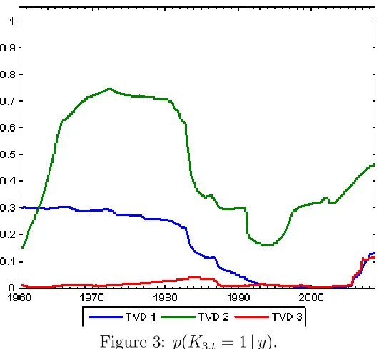
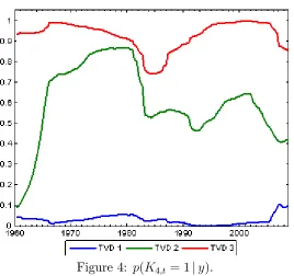
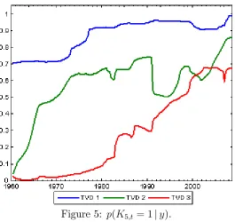
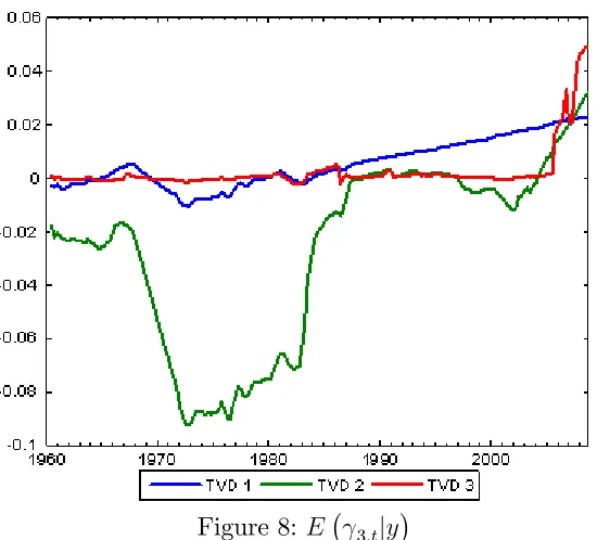
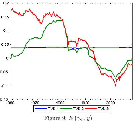
Remember that all of our models are speci…ed so that Kj;t = 1if the jth pre-dictor is included. Thus, the probability thatKj;t = 1sheds light on whether a predictor is included or excluded. In the latter case, a more parsimonious model is achieved. Figures 1 through 5 plotp(Kj;t = 1jy)for our three TVD models for j = 1; ::;5.

from the model. For instance, p(Kj;t = 1jy) = 0:2 does not totally exclude a predictor from the model, but shrinks its e¤ect towards zero.

Next consider the time varying aspect of the TVD models. Clearly there is substantial time variation in many of the lines in Figures 1 through 5, indicating that the impact of the corresponding predictor is changing over time. We can also be sure any patterns are not an artifact of the statistical methodology, since the patterns are so di¤erent in the di¤erent …gures. For instance, one might expect that the lines in the …gures would uniformly tend to increase over time since the available data is increasing, leading to more “signi…cant” coe¢ cients. This is not the case. Although there are some cases wherep(Kj;t = 1jy)is increasing over time, there are many where it is not. Similarly, although our use of hierarchical priors will ensure shrinkage, the patterns in the …gures do not solely re‡ect this shrinkage since some are shrunk much more than others. In short, these …gures indicate that our TVD models are capturing time variation in the coe¢ cients in a sensible and automatic fashion.

Next let us compare our three di¤erent TVD models. Broadly speaking, they are yielding similar results. However, our …rst TVD model is sometimes a bit di¤erent from the other two. It exhibits less time variation and, loosely speaking, tends to either include a variable or exclude it. This is not sur-prising in light of the properties of this model (see Section 2.2). That is, the longer a predictor is excluded from the model, the larger the variance in the state equation prior becomes (and the less shrinkage applies). This could be an attractive feature if there are big structural breaks for the co-e¢ cients. But, in our data set, this is a less attractive property. The third TVD approach shares these properties with the …rst TVD model, but this is partly counteracted by the added dimension reduction noted in Section 2.4. However, these considerations suggest that the second TVD approach might be most suitable for dealing with data sets with frequent small breaks.

TVD models).

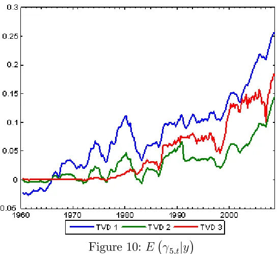
Figure 5: p(K5;t = 1jy).

Figure 10: E _5;tjy

3.7

Results: Forecasting Exercise

Our models provide us with p(y +1jData ), the predictive density for y +1

using data available through time . The predictive density is evaluated for

= 0; ::; T 1where 0 is 1969Q4. Let yo+1 be the observed value of y +1.

Mean squared forecast error and mean absolute forecast error are common measures of forecast performance. These are de…ned as:

M SF E =

PT 1 = 0 y

o

+1 E(y +1jData ) 2

T 0

and

M AF E=

PT 1 = 0 y

o

+1 E(y +1jData )

T 0

to evaluate forecast performance. Note that a great advantage of predictive likelihoods is that they evaluate the forecasting performance of the entire predictive density. Predictive likelihoods are motivated and described in many places such as Geweke and Amisano (2010). The predictive likelihood is the predictive density for y +1 evaluated at the actual outcome yo+1. We

use the sum of log predictive likelihoods for forecast evaluation:

T 1

X

= 0

log p y +1 =yo+1jData :

Note that, if 0 = 0 then this would be equivalent to the log of the marginal

likelihood. Hence, the sum of log predictive likelihoods can also be inter-preted as a measure similar to the log of the marginal likelihood, but made more robust by ignoring the initial 0 1observations in the sample (where

prior sensitivity is most acute).3

Table 2 presents these forecast metrics for our three TVD approaches, the TVP model, a random walk model, the constant coe¢ cient model (CC) and the constant coe¢ cient model with stochastic volatility (CCSV). Regardless of which forecast metric we use, the evidence of Table 2 strongly indicates that all of our TVD approaches are forecasting substantially better than commonly-used benchmarks. Note that the researcher may wish to use the sum of log predictive likelihoods to construct posterior model probabilities for use in a Bayesian model averaging (BMA) exercise. If the two models under consideration were the second TVD model and the heteroskedastic constant coe¢ cient model, then only 5% of the weight would be attached to the constant coe¢ cient model. The homoskedastic constant coe¢ cient model would receive only 1% in a similar exercise.

When we compare our three TVD approaches, we …nd that they perform similarly to one another. In terms of the predictive likelihoods (the met-ric preferred by most Bayesians), the second TVD approach forecasts best. However, in terms of MSFEs (MAFEs) the …rst (third) TVD approaches forecast best.

Table 2: Measures of Forecast Performance

Model MSFE MAFE Sum of log

Pred. like.

TVD 1 12.06 29.32 -8.96

TVD 2 13.13 30.02 -8.60

TVD 3 12.74 29.23 -8.62

Random Walk 27.37 41.08 –

CC 16.98 32.51 -13.10

CCSV 15.77 32.14 -11.50

TVP 13.74 31.01 -9.41

Figure 12: Cumulative Sums of Log Predictive Likelihoods

4

Conclusions

In this paper, we have presented a battery of theoretical and empirical ar-guments for the potential bene…ts of TVD models. Like TVP models, TVD models allow for the values of the parameters to change over time. Unlike TVP models, they also allow for the dimension of the parameter vector to change over time. Given the potential bene…ts of a TVD framework, the task is to build speci…c TVD models. This task was taken up in section 2 of this paper where three di¤erent TVD models were developed. These models all are dynamic mixture models and, thus, have the enormous bene…t that we can draw on existing methods of posterior computation developed in Gerlach, Carter and Kohn (2000).

References

Amato, J. and Swanson, N., 2001, The real-time predictive content of money for output, Journal of Monetary Economics, 48, 3-24.

Ang, A. Bekaert, G. and Wei, M., 2007, Do macro variables, asset mar-kets, or surveys forecast in‡ation better?, Journal of Monetary Economics

54, 1163-1212.

Ballabriga, F., Sebastian, M. and Valles, J., 1999, European asymmetries,

Journal of International Economics, 48, 233-253.

Canova, F., 1993, Modelling and forecasting exchange rates using a Bayesian time varying coe¢ cient model,Journal of Economic Dynamics and Control, 17, 233-262.

Canova, F., 2007, Methods for Applied Macroeconomic Research, Prince-ton University Press: PrincePrince-ton.

Canova, F. and Ciccarelli, M., 2004, Forecasting and turning point predic-tions in a Bayesian panel VAR model,Journal of Econometrics, 120, 327-359. Carter, C. and Kohn, R., 1994, On Gibbs sampling for state space models,

Biometrika, 81, 541–553.

Chan, J.C.C. and Jeliazkov, I., 2009, E¢ cient simulation and integrated likelihood estimation in state space models, International Journal of

Mathe-matical Modelling and Numerical Optimisation, 1, 101-120.

Chib, S., 1996, Calculating posterior distributions and modal estimates in Markov mixture models, Journal of Econometrics, 75, 79-97.

Chib, S. and Greenberg, E., 1995, Hierarchical analysis of SUR models with extensions to correlated serial errors and time-varying parameter mod-els, Journal of Econometrics, 68, 339-360.

Ciccarelli, M. and Rebucci, A., 2002, The transmission mechanism of European monetary policy: Is there heterogeneity? Is it changing over time?, International Monetary Fund working paper, WP 02/54.

Cogley, T. and Sargent, T., 2005, Drifts and volatilities: Monetary poli-cies and outcomes in the post WWII U.S., Review of Economic Dynamics, 8, 262-302.

D’Agostino, A., Gambetti, L. and Giannone, D., 2009, Macroeconomic forecasting and structural change, ECARES working paper 2009-020.

Durbin, J. and Koopman, S., 2002, A simple and e¢ cient simulation smoother for state space time series analysis, Biometrika, 89, 603-616.

Geweke, J. and Amisano, G., 2010, Hierarchical Markov normal mix-ture models with applications to …nancial asset returns, Journal of Applied

Econometrics, forthcoming.

Giordani, P. and Kohn, R., 2008, E¢ cient Bayesian inference for mul-tiple change-point and mixture innovation models, Journal of Business and Economic Statistics, 12, 66-77.

Giordani, P., Kohn, R. and van Dijk, D., 2007, A uni…ed approach to nonlinearity, structural change and outliers, Journal of Econometrics, 137, 112-133.

Groen, J., Paap, R. and Ravazzolo, F., 2009, Real-time In‡ation Fore-casting in a Changing World, Econometric Institute Report 2009-19, Erasmus University.

Kim, S., Shephard, N. and Chib, S., 1998, Stochastic volatility: likelihood inference and comparison with ARCH models, Review of Economic Studies, 65, 361-93.

Koop, G., 2003,Bayesian Econometrics, Wiley: Chichester.

Koop, G. and Korobilis, D., 2009, Forecasting in‡ation using dynamic model averaging, manuscript available at http://personal.strath.ac.uk/gary.koop/.

Koop, G., León-González, R. and Strachan R.W., 2009a, Dynamic prob-abilities of restrictions in state space models: An application to the Phillips curve, Journal of Business and Economic Statistics, forthcoming.

Koop, G., León-González, R. and Strachan R.W., 2009b, On the evolu-tion of the monetary policy transmission mechanism, Journal of Economic Dynamics and Control, 33, 997–1017.

Koop, G. and Potter, S., 2009, Time varying VARs with inequality

restric-tions, manuscript available at http://personal.strath.ac.uk/gary.koop/koop_potter14.pdf. Korobilis, D., 2009, VAR forecasting using Bayesian variable selection,

manuscript available at http://mpra.ub.uni-muenchen.de/21124/.

Primiceri. G., 2005, Time varying structural vector autoregressions and monetary policy, Review of Economic Studies, 72, 821-852.

Raftery, A., Karny, M., Andrysek, J. and Ettler, P., 2007, Online predic-tion under model uncertainty via dynamic model averaging: Applicapredic-tion to a cold rolling mill, Technical report 525, Department of Statistics, University of Washington.

Staiger, D., Stock, J. and Watson, M., 1997, The NAIRU, unemployment and monetary policy, Journal of Economic Perspectives, 11, 33-49.