promoting access to White Rose research papers
White Rose Research Online [email protected]
Universities of Leeds, Sheffield and York
http://eprints.whiterose.ac.uk/
This is the author’s post-print version of an article published in
Physical Review D
White Rose Research Online URL for this paper:
http://eprints.whiterose.ac.uk/id/eprint/76132
Published article:
Combes, F, Vega, HJD, Mikhailov, AV and Sánchez, N (1993)Multi-String Solutions by Soliton Methods in De Sitter Spacetime. Physical Review D, 50. 2754 - 2768. ISSN 0556-2821
arXiv:hep-th/9310073v1 13 Oct 1993
LPTHE 93-44
MULTI-STRING SOLUTIONS BY SOLITON METHODS IN DE SITTER SPACETIME
F. Combes(a), H.J. de Vega(b), A. V. Mikhailov(a,c) and N. S´anchez(a)
(a) Observatoire de Paris, Section de Meudon, Demirm, Laboratoire Associ´e au CNRS UA 336, Observatoire de Meudon et ´Ecole Normale Sup´erieure. 92195 MEUDON Principal
Cedex, FRANCE.
(b) Laboratoire de Physique Th´eorique et Hautes Energies, Universit´e Paris VI, Tour 16, 1er ´etage, 4, Place Jussieu 75252 Paris, Cedex 05, FRANCE.
(c) Landau Institute for Theoretical Physics, Russian Academy of Sciences, Ul. Kossyguina 2, 117334 Moscow, RUSSIA
Abstract
Exactsolutions of the string equations of motion and constraints aresystematically
constructed in de Sitter spacetime using the dressing method of soliton theory. The string dynamics in de Sitter spacetime is integrable due to the associated linear system. We start from an exact string solutionq(0)and the associated solution of the linear system Ψ(0)(λ), and we construct a new solution Ψ(λ) differing from Ψ(0)(λ) by a rational matrix inλwith at least four poles λ0,1/λ0, λ∗0,1/λ∗0. The periodicity condition for closed strings restrict
λ0 to discrete values expressed in terms of Pythagorean numbers. Here we explicitly construct solutions depending on (2 + 1)-spacetime coordinates, two arbitrary complex numbers (the ’polarization vector’) and two integers (n, m) which determine the string windings in the space. The solutions are depicted in the hyperboloid coordinatesq and in comoving coordinates with the cosmic time T . Despite of the fact that we have a single world sheet, our solutions describemultiple(here five) different and independent strings; the world sheet timeτ turns to be a multivalued function ofT. (This has no analogue in flat spacetime). One string is stable (its proper size tends to a constant for T → ∞, and its comoving size contracts); the other strings are unstable (their proper sizes blow up for
1
Introduction
Since the propagation of strings in curved spacetimes started to be systematically investi-gated, a variety of new physical phenomena appeared [1]-[2]. These results are relevant both for fundamental (quantum) strings and for cosmic strings which behave essentially in a classical way.
String propagation has been investigated in non-linear gravitational plane waves [3] and shock-waves [4], black holes [5], conical spacetimes [6], and cosmological spacetimes [1],[7].
Among the cosmological backgrounds, de Sitter spacetime occupies a special place. This is, in one hand relevant for inflation and on the other hand string propagation turns to be specially interesting there [1],[7]. String unstability, in the sense that the string proper length grows indefinitely is particularly present in de Sitter. The string dynamics in de Sitter universe is described by a generalized sinh-Gordon model with a potential unbounded from below [14]. The sinh-Gordon function α(σ, τ) having a clear physical meaning : H−1eα(σ,τ)/2 determines the string proper length. Moreover the classical string equations of motion (plus the string constraints) turn to be integrable in de Sitter universe [14],[15]. More precisely, they are equivalent to a non-linear sigma model on the grassmannian SO(D,1)/O(D) with periodic boundary conditions (for closed strings). This sigma model has an associated linear system [8] and using it, one can show the presence of an infinite number of conserved quantities [12]. In addition, the string constraints imply a zero energy-momentum tensor and these constraints are compatible with the integrability.
The so-called dressing method [8] in soliton theory allows to construct solutions of non-linear classically integrable models using the associated non-linear system. In the present paper we systematically construct string solutions in three dimensional de Sitter spacetime. We start from a given exactly known solution of the string equations of motion and constraints in de Sitter [15] and then we “dress” it. The string solutions reported here indeed apply to cosmic strings in de Sitter spacetime as well. The dynamics of cosmic strings in expanding universes has been studied in the literature for the Friedman-Robertson-Walker (FRW) cases (see for example [9], [10],[16]). It must be noticed that the string behaviour we found here in de Sitter universe is essentially different from the standard FRW where the expansion factor R(T) is a positive power of the cosmic time T. In such FRW universes, strings always oscillate in time, the comoving spatial string coordinates contract and the proper string size stays constantasymptotically forT → ∞[7],[16] . In the cosmic string literature this is known as ’string stretching’. We called such behaviour ’stable’ [7],[15],[16]. On the contrary, in de Sitter spacetime, as we show below, two types of asymptotic behaviors are present : (i) the proper string size and energy grow with the expansion factor (’unstable’ behaviour) or (ii) they tend to constant values (’stable’ strings).
inflation as proposed in refs.[11]-[7] without advocating an inflaton field. The multi-string exact solutions in de Sitter spacetime presented here should provide essential clues about the feasability of inflationary string scenarios.
We apply here the dressing method as follows. We start from the exact ring-shaped string solutionq(0) [15] and we find the explicit solution Ψ(0)(λ) of the associated linear system, where
λ stands for the spectral parameter. Then, we propose a new solution Ψ(λ) that differs from Ψ(0)(λ) by a matrix rational inλ. Notice that Ψ(λ= 0) provides in general a new string solution. We then show that this rational matrix must have at least four poles, λ0,1/λ0, λ∗0,1/λ∗0, as a consequence of the symmetries of the problem. The residues of these poles are shown to be one-dimensional projectors. We then prove that these projectors are formed by vectors which can all be expressed in terms of an arbitrary complex constant vector |x0i and the complex parameter λ0. This result holds for arbitrary starting solutions q(0).
Since we consider closed strings, we impose a 2π-periodicity on the string variable σ . This restrictsλ0to take discrete values that we succeed to express in terms of Pythagorean numbers. In summary, our solutions depend on two arbitrary complex numbers contained in|x0iand two integersnandm. The counting of degrees of freedom is analogous to 2+1 Minkowski spacetime except that left and right modes are here mixed up in a non-linear and precise way.
The vector |x0isomehow indicates the polarization of the string. The integers (n, m) deter-mine the string winding. They fix the way in which the string winds around the origin in the spatial dimensions (hereS2 ). Our starting solutionq(0)(σ, τ) is a stable string winded n2+m2 times around the origin in de Sitter space.
The matrix multiplications involved in the computation of the final solution were done with the help of the computer program of symbolic calculation “Mathematica”. The resulting solution q(σ, τ) = (q0, q1, q2, q3) is a complicated combination of trigonometric functions of σ and hyperbolic functions ofτ. That is, these string solitonic solutions do not oscillate in time. This is a typical feature of string unstability [5]-[7]-[15]. The new feature here is that strings (even stable solutions) do not oscillate neither for τ → 0, nor for τ → ±∞. Figs. 3-4 depict spatial projections (q1, q2, q3) of the solutions for two given polarizations |x
0i and different windings (m, n).
We plot in figs. 5-11 the solutions for significative values of |x0i and (m, n) in terms of the comoving coordinates (T, X1, X2)
T = 1
H log(q
0+q1) , X1 = 1
H
q2
q0 +q1 , X
2 = 1
H
q3
q0+q1 (1)
always be chosen proportional to τ. In flat spacetime, multiple string solutions are described by multiple world-sheets. Here, we have a single world-sheet describing several independent and simultaneous strings as a consequence of the coupling with the spacetime geometry. Notice that we consider free strings. (Interactions among the strings as splitting or merging are not considered). Five is the generic number of strings in our dressed solutions. The value five can be related to the fact that we are dressing a one-string solution (q(0)) with four poles. Each pole adds here an unstable string.
In order to describe the real physical evolution, we eliminated numericallyτ =τ(σ, T) from the solution and expressed the spatial comoving coordinates X1 and X2 in terms ofT and σ.
We plotτ(σ, T) as a function ofσ for different fixed values of T in fig.7-8. It is a sinusoidal-type function. Besides the customary closed string period 2π, another period appears which varies onτ. For small τ ,τ =τ(σ, T) has a convoluted shape while for largerτ (here τ ≤5), it becomes a regular sinusoid. These behaviours reflect very clearly in the evolution of the spatial coordinates and shape of the string.
The evolution of the five (and three) strings simultaneously described by our solution as a function of T, for positive T is shown in figs. 9-11. One string is stable (the 5th one). The other four are unstable. For the stable string, (X1, X2) contracts in time precisely as e−HT,
thus keeping the proper amplitude (eHTX1, eHTX2) and proper size constant. For this stable string (X1, X2) ≤ 1
H. (1/H = the horizon radius). For the other (unstable) strings, (X
1, X2) become very fast constant in time, the proper size expanding as the universe itself like eHT
. For these strings (X1, X2) ≥ 1
H. These exact solutions display remarkably the asymptotic
string behaviour found in refs.[7],[14].
In terms of the sinh-Gordon description, this means that for the strings outside the horizon the sinh-Gordon functionα(σ, τ) is the same as the cosmic timeT up to a function ofσ. More precisely,
α(σ, τ)T >> 1 H
= 2H T(σ, τ) + logn2H2h(A1(σ)′)2 + (A2(σ)′)2io+O(e−2HT). (2) Here A1(σ) and A2(σ) are the X1 and X2 coordinates outside the horizon. For T → +∞ these strings are at the absolute minimun α = +∞ of the sinh-Gordon potential with infinite size. The string inside the horizon (stable string) corresponds to themaximunof the potential,
α = 0. α = 0 is the only value in which the string can stay without being pushed down by the potential to α = ±∞ and this also explains why only one stable string appears (is not possible to put more than one string at the maximun of the potential without falling down). These features aregenericallyexhibited by our one-soliton multistring solutions, independently of the particular initial state of the string (fixed by|x0 > and (n, m)). For particular values of |x0 >, the solution describes three strings, with symmetric shapes fromT = 0, for instance like a rosette or a circle with festoons (fig. 9-11).
de Sitter universe. Moreover, the construction method used here works in any number of dimensions.
This paper is organised as follows: in section 2 we describe the string equations in de Sitter universe and its associated linear system. Section 3 deals with the dressing method in soliton theory, its application to this string problem and the systematic construction of solutions. In section 4 we explicitly describe the starting background solution q(0)(σ, τ) and the solution Ψ(0)(λ) of the associated linear system. In section 5, we analyze our multistring solutions and describe their physical properties.
2
The string equations and their associated linear
sys-tem
The string equations of motion in D-dimensional de Sitter space-time can be written in the following form:
qξηi+qihqξJqηi= 0, (3)
where qi is a (D+ 1)-dimensional real vector of unit pseudolength
hqJqi= 1, (J = diag(−1,1, ...,1)) (4) and ξ, η are light cone coordinates in the world sheet:
τ =η+ξ, σ =η−ξ (5)
In addition, we have the string constraints (conformal conditions)
hqξJqξi= 0, hqηJqηi= 0. (6)
The solution qi should be a periodic function ofσ =η−ξ, with period 2π for closed strings. We are going to find solutions of this equation by using the Riemann Transform Method [8, 13]. The most important observation is that equation (3) can be rewritten in the form of a chiral field model on the GrassmanianGD =SO(D,1)/O(D).Indeed, any elementg ∈GD can
be parametrized with a real vector qi of the unit pseudolength
g= 1−2qihqJ, hqJqi= 1. (7) In terms of g, the string equations (3)-(6) have the following form
and the conformal constraints are
trg2ξ = 0, trg2η = 0 , (9) which are equivalent to eqs.(6). The fact thatg ∈GD implies that g is a real matrix with the
following properties:
g=JgtJ, g2 =I, trg= 2 g ∈SL(D+ 1, R). (10) These conditions are equivalent to the existence of the representation (7).
Equation (8) is the compatibility condition for the following overdetermined linear system:
Ψξ =
U
1−λΨ, Ψη = V
1 +λΨ, (11)
where
U =gξg, V =gηg . (12)
Or in terms of vector qi
U = 2qξihq J −2qihqξJ,
V = 2qηihq J −2qihqηJ.
In order to fix the freedom in the definition of Ψ we shall identify
Ψ(λ= 0) =g. (13)
This condition is compatible with the above equations since the matrix function Ψ at the pointλ= 0 satisfies the same equations as g. Thus the problem of constructing exact solutions of the string equations is reduced to finding compatible solutions of the linear equations (11) such that g= Ψ(λ= 0) satisfies the constraints eqs.(9) and (10).
3
The Dressing Method in Soliton Theory
3.1
The reduction group of the associated linear system
We will consider now the symmetry group (or the so called “reduction group” [8], [13]) enjoyed by the linear system of equations
Ψξ =
U
1−λΨ, Ψη = V
1 +λΨ, (14)
It follows from the condition hqJqi= 1 that the matrixg =I−2qihgJ anticommutes with
U and V:
gU +Ug = 0, gV +Vg= 0.
This implies that the matrix function gΨ(1/λ) satisfies the same equation as Ψ(λ) :
[gΨ(1/λ)]ξ=
U
1−λ[gΨ(1/λ)], [gΨ(1/λ)]η = V
1 +λ[gΨ(1/λ)], (15)
Then, it can differ from Ψ(λ) only on a matrix multiplier which does not depend on ξ, η:
gΨ(1/λ) = Ψ(λ)δ1(λ). (16) The vector qi, the corresponding matrix gand the currents U, V are real. Therefore Ψ∗(λ∗) is a solution of equations (11) as well, and we have
Ψ∗(λ∗) = Ψ(λ)δ2(λ) (17) In addition, by using eq.(17) twice, we find
δ2(λ) δ2∗(λ∗) =I (18)
The fact that g∈SO(3,1) yields JUTJ =−U, JVTJ =−V and implies that (JΨt(λ)J)−1 obeys the same equation (11) as Ψ(λ)
(JΨt(λ)J)−1 = Ψ(λ)δ
3(λ). (19)
The transformations (16),(17) and (19) generate a finite group which is called the reduction group of the problem and which guarantees that the properties (10) hold for g= Ψ(λ = 0).
3.2
Rational dressing
Suppose we know a particular solutiong(0)(η, ξ) of the string equations (3). We shall denote by U(0)(η, ξ), V(0)(η, ξ) its corresponding currents (12), and by Ψ(0)(λ, η, ξ) , the corresponding compatible solution of the overdetermined system (11). We assume that Ψ(0) as well as U
(0) and V(0) are explicitly known.
To construct a new solution g we assume that the corresponding Ψ function differs from Ψ(0) on a rational matrix multiplier Φ(λ, η, ξ)
the linear system (14) and the symmetry conditions (16)-(19). Then, once Φ(λ) is known, the string solution g(η, ξ) follows from eq.(13).
It follows from (13),(16) and (20) that Φ should obey the following symmetries:
Φ(0)Ψ(0)(0)Φ(1/λ) = Φ(λ)Ψ(0)(0), (21)
Φ∗(λ∗) = Φ(λ), (22)
JΦt(λ)J = Φ−1(λ) (23)
We assume that the constant matrices δ1(λ), δ2(λ) and δ3(λ) coincide for the dressed and the undressed solutions.
Suppose that the rational function Φ(λ) has a pole at the point λ0. It follows from eqs.(21) and (22) that it must have poles at the points 1/λ0, λ∗0,1/λ∗0as well and, in addition, Φ(∞) =I. Thus, the simplest (generic) possible case is
Φ(λ) =I + A
λ−λ0
+ A ∗
λ−λ∗
0
+ B
λ−λ−10 +
B∗
λ−λ∗−10 (24)
where A, B are matrix functions of (ξ, η) to be determined below. This simplest case will be called the one-soliton solution from now on. We choose this name since in the context of non-linear integrable equations in an infinite space interval (the sine-Gordon equation, for instance), this minimal pole-structure (the minimal number of poles compatible with the symmetry group) inλ generates the one soliton solution (see for example [17]).
Here we have taken into account eqs.(22) and (21). It follows from eq. (23) that
Φ−1(λ) =I+ JA tJ
λ−λ0
+ JA †J
λ−λ∗
0
+ JB tJ
λ−λ−10
+ JB †J
λ−λ∗−10
(25) here † denotes Hermitian conjugation of a matrix. The condition Ω(λ) = Φ(λ)Φ−1(λ) =I can be imposed in the following way: the right hand side (Ω(λ)) is a rational function of λ which takes the value I at the point λ = ∞, then Ω(λ) will be identically I if it does not have any singularity on the Riemann sphere of λ. Double poles would vanish if and only if
AJAt = 0, BJBt = 0. (26)
Thus the matrices A, B are degenerated and we can write them as a sum of bivectors
A=X
i
aiihxiJ, B =
X
i
biihyiJ. (27)
The constraints (26) imply
hxi|J|xji= 0 for all pairs i,j. (28)
which means that the vectors xii are null and mutually pseudo-orthogonal. Therefore, since
pseudo-orthogonal null vectors are proportional, we have
and without loss of generality, we take:
A=aihxJ, B =bihyJ. (29)
Now the constraints (26) read
hxJxi= 0, hyJyi= 0 (30)
In addition, by requiring the residues of Ω(λ) to vanish at the points λ0,1/λ0, λ∗0, 1/λ∗0 , we get
AJ+JAt +AJ( B
t
λ0−λ−10
+ A
†
λ0−λ∗0
+ B
†
λ0−λ∗−10
) + ( BJ
λ0 −λ−10
+ A ∗J
λ0−λ∗0
+ B
∗J
λ0−λ∗−10
)At = 0
BJ+JBt +BJ(− A
t
λ0 −λ−10
+ B
†
λ−10 −λ∗−10
+
A†
λ0−λ∗−10
) + (− AJ
λ0 −λ−10
+ B
∗J
λ−10 −λ∗−10 +
A∗J
λ0−λ∗−10
)Bt = 0
A∗J+JA†+A∗J( B
†
λ∗
0−λ∗−10
+ A
t
λ∗
0−λ0
+ B
t
λ∗
0−λ−10
) + ( B ∗J
λ∗
0−λ∗−10
+ AJ
λ∗
0 −λ0
+ BJ
λ∗
0−λ−10
)A† = 0
B∗J +JB†+B∗J(
− A
†
λ∗
0−λ∗−10
+ Bt
λ∗−10 −λ−10
+ At
λ∗
0−λ−10 ) +
(− A ∗J
λ∗
0−λ∗−10
+ BJ
λ∗−10 −λ−10
+ AJ
λ∗
0−λ−10
)B†= 0
Later on we shall demonstrate that the periodicity condition on σ can be satisfied only in the case where all poles (λ0, λ∗0, λ−10 , λ∗−10 ) of Φ(λ) are purely imaginary [see eqs.(59),(68) and (70)]. From now on, we shall denoteλ0 =iκ, κ∈R. Substituting the bivectoral representation (29) in the above equations and by separating bivectors we get the system of vector equations with respect to ai, bi
biihxJyi
κ+κ−1 +a
∗ iihx
∗Jxi 2κ +b
∗ iihy
∗Jxi
κ−κ−1 = xi
b∗iihx
∗Jy∗ i
κ+κ−1 +ai
ihx∗Jx
i 2κ +bi
ihx∗Jy
i
κ−κ−1 = −x
∗ i
−ai ihxJyi
κ+κ−1 −b
∗ iihy
∗Jy i 2κ−1 +a
∗ iihx
∗Jy i
κ−κ−1 = yi
−a∗ iihx
∗Jy∗i
κ+κ−1 −bi
ihy∗Jyi
2κ−1 +ai
ihy∗Jxi
κ−κ−1 = −y
∗ i
By bivectoral separations we mean the following trick: suppose ve have an equation of the form
One can solve this system of linear equations and express the vectors ai, biin terms ofxi, yi
ai = 2iκ(κ
4−1)
δ [(κ
4
−1)x∗
ihy∗Jy
i+ 2(1 +κ2)y∗
ihx∗Jy
i+ 2(1−κ2)yihx∗Jy∗
i] (31)
bi = 2i(κ
4−1)
κδ [(κ
4
−1)y∗
ihx∗Jx
i+ 2κ2(1 +κ2)x∗
ihy∗Jx
i+ 2κ2(1−κ2)xihx∗Jy∗ i] (32) where δ is the scalar function
δ = (1−κ4)2hx∗Jx
ihy∗Jy
i+ 4κ2(1 +κ2)2hx∗Jy
ihy∗Jx
i −4κ2(1−κ2)2hx∗Jy∗
ihxJyi (33) At the moment we have fulfiled the reduction constraints (22), (23) completely, but the con-straint eq.(21) has not yet been imposed. One can prove without loose of generality, that eq.(21) is verified, when the vectors xi, yi, fulfil
yi= Ψ(0)(0)xi. (34)
Assembling eqs.(29) and eqs.(31)-(34) all together one can find Φ (eq.(24)) as a function of
xi, λ, λ0
Φ = Φ(λ, λ0, xi) (35)
Now, we are interested in the value of this function at λ = 0, since it gives a new solution
g= Φ(0)g(0). One can check that
g = g(0)−
4(1−κ4)
δ [(1−κ
4)(Fg
(0)+g(0)F)hx∗Jxi+ (36)
2(1 +κ2)(κ2F −g(0)Fg(0))hx∗Jg
(0)xi −2(1−κ2)Re((κ2H+g(0)Hg(0))hx∗Jg(0)x∗i)], where
F = Re(x∗
ihxJ), H =xihxJ
Thus, we have parametrised the new solution g by a real number κ and a complex vector
xi of zero pseudolength. Sinceg satisfies the conditions (10), it has the form of eq.(7) and the corresponding vectorqi, can be found by projecting eq.(7) on an arbitrary constant vector pi. (For instance (1,0,0,0)). We find in this way:
qi= q pi −gpi
3.3
Evolution of
x
i
and
κ
in
ξ
and
η
.
Now the problem is to find the evolution of xi and κ in ξ and η. It follows from eqs.(11), (20) that
Φξ+
1
1−λΦU(0) =
1
1−λUΦ, (38)
Φη +
1
1 +λΦV(0) =
1
1 +λVΦ, (39)
where U, V are still undetermined functions of η, ξ which do not depend on λ. Let us rewrite equations (38), (39) in the form
Φ(−∂ξ+
U(0)
1−λ)Φ
−1 = U
1−λ, (40)
Φ(−∂η+
V(0)
1 +λ)Φ
−1 = V
1 +λ. (41)
Consider the l.h.s. of (40). It is a rational function of λ with a pole at λ = 1 and at λ ∈
{λ0, λ−10 , λ∗0, λ∗−10 } , but the r.h.s. has only one pole at λ = 1 . Thus to fit eq.(40) we have to set the residues at λ0, λ−10 , λ∗0 and λ∗−10 equal to zero. In fact, it is sufficient to require the vanishing of the residue at λ0 only. All other residues will vanish due to the action of the reduction group. The condition
res|λ0Φ(−∂ξ+
U(0)
1−λ)Φ
−1 = 0 (42)
yields
A(∂ξ−
U(0)
1−λ0
)JAt = 0 (43)
and
A(∂ξ−
U(0)
1−λ0
)J( Bt
λ0 −λ−10
+ A
†
λ0−λ∗0
+ B
†
λ0−λ∗−10
) +
( B
λ0−λ−10
+ A
∗
λ0−λ∗0
+ B
∗
λ0−λ∗−10
)(∂ξ−
U(0)
1−λ0
)JAt = 0 (44) Both equations will be satisfied if
(∂ξ−
U(0)
1−λ0
)xi= 0 (45)
Thus, the simultaneous solution of eqs.(43) and (44) is
xi= Ψ(0)(η, ξ;λ0)x0i (46)
wherex0iis any complex constant vector of zero pseudolength, andλ0 turns not to depend on
Moreover, the solution (46) of equation (42) is also a solution of the equation
res|λ0Φ(−∂η +
V(0)
1 +λ)Φ
−1 = 0. (47)
Finally, the η, ξ dependance of the vector xi is given by eq.(46). Together with eq.(36) it gives the one soliton solution.
The wave function Ψ(η, ξ;λ) corresponding to the one soliton solution (let us denote it by Ψ1(η, ξ;λ) can be regarded as a function ofλ, λ0,Ψ(0)(η, ξ, λ), and x0i (see eqs.(20) and (35)). Ψ1(η, ξ;λ) = Φ(λ, λ0, JΨ(0)(η, ξ;λ0)Jx0i)Ψ0(η, ξ;λ) (48) The wave function corresponding to a n-soliton solution can be obtained recursively through the relation
Ψn(η, ξ;λ) = Φ(λ, λn−1, JΨn−1(η, ξ;λn−1)Jxn−1i)Ψn−1(η, ξ;λ), (49)
and the corresponding solution of the chiral model g = Ψn(η, ξ;λ = 0) will satisfy all the
reduction conditions eqs.(16),(17) and (19).
4
The choice of the background solution
Let us construct now explicit solutions by applying the above procedure . To begin with we shall consider a three dimensional de Sitter spacetime (D= 3).
As a background starting solution we choose for simplicity the solution q(0)(σ, τ) found in ref.[15]. This solution corresponds to the trivial α = 0 solution of the sinh-Gordon equation and it is given by,
q(0) =
1 √ 2 sinhτ coshτ cosσ sinσ
, q(0)ξ =
1 √ 2 coshτ sinhτ sinσ
−cosσ
, (50)
q(0)η =
1 √ 2 coshτ sinhτ
−sinσ
cosσ
, b(0) =
1 √ 2 sinhτ coshτ
−cosσ
−sinσ
, (51)
For this solution, we have
hq(0)ξJq(0)ηi=−1, hq(0)Jq(0)i= 1, hb(0)Jb(0)i= 1, otherh·J·i= 0
U(0) = 2q(0)ξihq(0)J−2q(0)ihq(0)ξJ, V(0) = 2q(0)ηihq(0)J−2q(0)ihq(0)ηJ
where J is given by eq.(4). Let us define
Q(ξ, η) = (q(0)ξ, q(0)η, q(0), b(0)) , (52) then we find by direct calculation that
QTJQ=
0, −1, 0, 0 −1, 0, 0, 0 0, 0, 1, 0 0, 0, 0, 1
U(0)Q= (0,2q(0),2q(0)ξ,0), V(0)Q= (2q(0),0,2q(0)η,0)
and
QTJU
(0)Q=
0, 0, 0, 0 0, 0, −2, 0 0, 2, 0, 0 0, 0, 0, 0
, QTJV
(0)Q=
0, 0, −2, 0 0, 0, 0, 0 2, 0, 0, 0 0, 0, 0, 0
QTJQξ =
0, 0, 0, −1 0, 0, −1, 0 0, 1, 0, 0 1, 0, 0, 0
, QTJQη =
0, 0, −1, 0 0, 0, 0, −1 1, 0, 0, 0 0, 1, 0, 0
We have to solve two compatible equations for Ψ
Ψ(0)ξ = U(0) 1−λΨ
(0), Ψ(0)
η =
V(0)
1 +λΨ
(0). (53)
Let us make the gauge transformation
Ψ(0) =Q(ξ, η) Ξ(ξ, η), (54) then
QTJQξΞ +QTJΞξ =
QTJU(0)Q
1−λ Ξ , Q
TJQ
ηΞ +QTJQΞη =
QTJV(0)Q
1 +λ Ξ , (55)
Ξξ=
0, 0, µ−2, 0 0, 0, 0, −1 0, µ−2, 0, 0 −1, 0, 0, 0
Ξ(ξ, η) (56)
Ξη =
0, 0, 0, −1 0, 0, µ2, 0
µ2, 0, 0, 0
0, −1, 0, 0
Ξ(ξ, η) (57)
(58) The solution will be defined on the Riemann surface Γ which covers twice the complex plane
λ:
µ2 = 1−λ
1 +λ (59)
The points λ=±1 are the branching points of Γ.
The fundamental set of solutions of eqs.(56)-(58) is given by:
exp(µη+µ−1ξ)
−µ−1 −µ −1 1
, exp(−µη−µ−1ξ)
µ−1 µ −1 1 , (60)
exp(iµη−iµ−1ξ)
iµ−1 −iµ 1 1
, exp(−iµη+iµ−1ξ)
−iµ−1
iµ 1 1 . (61)
It will be convenient to use the following linear combinations of the above solutions:
Ξ(µ, ξ, η) = Λ(µ).Π(µ, ξ, η) (62)
where:
Λ(µ) = diag(µ−1, µ,1,1) (63)
Π(µ, ξ, η) = √1
2
coshγ, −sinhγ, sinθ, −cosθ
coshγ, −sinhγ, −sinθ, cosθ
sinhγ, −coshγ, −cosθ, −sinθ
−sinhγ, coshγ, −cosθ, −sinθ
and
θ =µη− 1
µξ , γ =µη+
1
µξ (65)
Thus, Ψ(0)(µ, ξ, η) as expressed by
Ψ(0)(µ, ξ, η) =Q(ξ, η).Λ(µ).Π(µ, ξ, η) (66)
is the solution of the system (53) fulfilling the constraint (13) for the solution q(0). That is :
Ψ(0)(µ= 1, ξ, η) = 1−2|q
(0) >< q(0)|J.
We want solutions periodic in σ with period 2π. We see from eq.(62)-(66) that we have hyperbolic functions on the argument
σ
2(µ−µ
−1) + τ
2(µ+µ
−1) (67)
and trigonometric functions with the argument
σ
2(µ+µ
−1) + τ
2(µ−µ −1)
The solution to the σ-periodicity condition requires to have
µ= exp[iα] (68)
with real α and cosα and sinα to be rational numbers. The general solution is given by the Pythagorean numbers:
cosα= m 2−n2
m2+n2 , sinα=−
2mn
m2+n2 , m, n = integers (69) That is,
µ= m+in
m−in , m, n = integers (70)
We get in this way solutions with period 2π(m2 +n2) in σ. Upon the rescaling:
σ →σ(m2+n2) , τ →τ(m2 +n2), (71)
5
The soliton string solutions and their properties
We have now all the elements to obtain the explicit expression for the solution |q(η, ξ)i of the string eqs.(3)-(6). The explicit expression for the solution Ψ(0)(η, ξ;µ0) given by eq.(66) can be directly obtained by computing the indicated matrix multiplication; Q(η, ξ) is given by eqs.(50-52); Λ(µ) and Π(µ, ξ, η) are given by eqs.(64). This was done with the help of the computer program of symbolic calculation “Mathematica”.
By projecting Ψ(0)(η, ξ;µ0) thus obtained on a constant and complex null vextor |x
0i , we have directly the vector |xi. The matrix g(ξ, η) is obtained from eq.(36) also using “Mathe-matica”. Finally, the explicit solution|q(η, ξ)iis obtained by insertingg(ξ, η) in eq.(37). These string solutions depend on one complex parameterµthat depends on two integers nandm(see eq.(70)), and one complex null vector x0i , that is, three complex independent numbers. Only two independent complex components remain in fact since g(ξ, η) is homogeneous in x0i. As can be seen in eq.(36) , the changex0i →c x0iwherecis a complex number, leaves the solution invariant. The dependence on x0i is precisely like what happens for strings in D-dimensional Minkowski space-time, in which the solution depends on 2(D−2) complex coefficients. They account for the (D−2)-transverse degrees of freedom and for the two helicity modes (right and left movers) . Here, we are in three space-time dimensions and so we obtain two complex coefficients corresponding to the transverse degrees of freedom.
It can be noticed, that the linear system (14) fulfilled by Ψ(η, ξ, λ) is invariant under con-formal transformations on ξ, η . Thus the dressing transformations do not generate conformal modes but only physical (transverse) modes.
The vector x0i describes the polarization of the string; the integers m, nassociated to the
σ periodicity, label the string modes. In Minkowski space-time, only one integer labels the right-modes and another one labels the left-modes. Here, we obtain two independent integers for each mode. Notice that our modes combine left and right movers in a non-linear and precise way.
The resulting solution q(σ, τ) = (q0, q1, q2, q3) is a complicated combination of trigonomet-ric functions of σ and hyperbolic functions of τ . From eqs.(67)-(70), we see that we have trigonometric functions on the arguments
σ 2mn
m2 +n2 and σ
m2−n2
m2+n2
and hyperbolic functions on the arguments
τ 2mn
m2 +n2 and τ
m2−n2
m2+n2 (72)
accelerated expanding like de Sitter, and in black holes. The new feature here is that the string does not oscillate in time, neither for τ → 0 nor for τ → ±∞. It can be noticed that in decelerated expanding backgrounds, as it is the case in the standard Friedman-Robertson-Walker (FRW) expansion, string instability does not occur and the string behaviour is oscillating in τ [7]. This was recently confirmed for all values of τ, in the FRW universe, where explicit string solutions has been found [16]. The non-oscillatory behavior in time can be understood from the fact that the string motion in de Sitter spacetime reduces to a sinh-Gordon equation with negative potential [14]. In D = 3, this is precisely the standard sinh-Gordon equation, whose potential unbounded from below (see fig. 1) is responsible of the instability. By defining
eα(σ,τ)=−qξ.qη , (73)
the string equations (3) and string constraints (6) in de Sitter spacetime can be reduced to the sinh-Gordon equation
ατ τ −ασσ−eα+e−α = 0 (74)
Therefore, in order to find a solution in D = 3 de Sitter spacetime, one can start from a
σ-periodic solution of the sinh-Gordon equation (74) and insert it in the string equations (3):
h
∂τ2−∂σ2 −eα(σ,τ)iq(σ, τ) = 0 (75) Then, one must solve the linear equation (75) in q(σ, τ) and impose the constraints (4) and (6). This is actually an alternative method to the dressing method, to obtain string solutions in de Sitter spacetime.
The function eα(σ,τ) has a clear physical interpretation, as it determines the proper string size. The invariant interval between two points on the string, computed with the spacetime metric, is given by
ds2 = 1
H2dq.dq =
1 2H2 e
α(σ,τ) (dσ2
−dτ2) (76)
The energy density of the sinh-Gordon model here H= 1
2 [ (
∂α
∂τ)
2+ (∂α
∂σ)
2 ]
−2 coshα(σ, τ), (77) determines the potential
Vef f =−2 coshα , (78)
This potential has absolute minima at α = +∞ and α =−∞. As the time τ evolves, α(σ, τ) generically approach one of these infinite minima. The first minimun corresponds to an infinitely large string whereas the second one describes a collapsed configuration. That is, the string in de Sitter spacetime will tend generically either to inflate (when α →+∞) or to collapse to a point (when α→ −∞).
sinh-Gordon model this corresponds to a particle at the maximun of the potential Vef f = −2
and with zero velocity.
Let us recall that for a given time q0, the de Sitter space is a sphere S2 with radius
R = 1
H
q
1 +q2
0 . For the background solution q(0)(σ, τ) given by eq.(50), we have R(τ) = 1
H
q
1 + 12sinh2τ. As de Sitter universe expands for τ → ∞ , the string size eα(σ,τ) = 1 remains here constant. This solution is probably unstable under small perturbations.
It must be noticed that the integers (m, n) of the solitonic solutions (69) have the meaning of string winding. They label the different ways in which the string wind in the spatial compact dimensions (here S2). Notice that our string solutions do not oscillate in time in spite of the fact that we are in a lorentzian signature spacetime. (The dependence on τ is hyperbolic).
In figs. 3 and 4 we plot the one soliton solutions |q(σ, τ)i = (q0, q1, q2, q3) found here. They show the three dimensional spatial projections (q1, q2, q3) as a function of σ, for a given polarization vectorx0i, different values ofm, n and two differents values ofτ. Figs. 3a and 3b show the same solution (n= 2, m= 1, x0i= (1,−1, .1, .1i)) for two different values of τ. Figs. 4a and 4b show the evolution for a higher winding number (n = 5), and polarization vector
x0i= (1,−1,1, i).
For comparison, let us recall, that in D = 2 spacetime dimensions, in which the string motion reduces to the Liouville equation, the exact general solution is a string wound n times around the de Sitter space and evolving with it. The string covers n times de Sitter space which is here a circle S1. This solution is given by [14]
q0 =−cotnτ , q1 = cosnσ
sinnτ , q
2 = sinnσ
sinnτ (79)
0< σ≤2π , 0< τ ≤π/n (80)
The invariant interval between two points of the string
ds2 = 1
H2sin2nτ(dσ2−dτ2) (81)
exhibits the typical feature of string instability : in the asymptotic regionsτ →0+andτ →π/n, the proper string length blows up. We also see that the string does not have “enough time” to oscillate in one expansion time of the universe : the oscillation period of the string coincides
with the expansion time of the universe. When the string accomplishes one oscillation, the universe has ended.
In order to analyze the exact solutions |q(σ, τ)i , it is convenient to use the coordinates (T, X1, X2) in this 2 + 1-dimensional de Sitter spacetime:
q0 = sinhHT +H2
2 exp(HT)
h
(X1)2+ (X2)2i
(82)
q1 = coshHT −H
2
2 exp(HT)
h
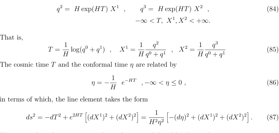
q2 = Hexp(HT)X1 , q3 = Hexp(HT) X2 , (84)
−∞< T, X1, X2 <+∞.
That is,
T = 1
H log(q
0+q1) , X1 = 1
H
q2
q0 +q1 , X
2 = 1
H
q3
q0+q1 (85)
The cosmic time T and the conformal time η are related by
η =− 1
H e
−HT ,
−∞< η ≤0 , (86)
in terms of which, the line element takes the form
ds2 =−dT2+e2HTh
(dX1)2+ (dX2)2i
= 1
H2η2
h
−(dη)2+ (dX1)2+ (dX2)2i
. (87)
We now analyze the properties and new features exhibited by these solutions.
[image:20.612.55.537.72.303.2]First of all, let us analyze the cosmic time coordinate T =T(σ, τ). We have studied T as a function of τ for different fixed values of σ and viceversa. These functions have been obtained numerically for a wide family of solutions labeled by different values of the parametersn, mand |x0i. We report here only two significative cases, which show the genericfeatures, irrespective of the particular values of these parameters.
Fig. 5 shows T as a function of τ for the values of σ indicated in the picture. We depict T
for n= 4, m= 1 and a generic|x0i= (1 +i, .6 +.4i, .3 +.5i, .77 +.79i).
In fig. 6 we depict T as a function of τ for the solution with n = 4, m = 1 and |x0i = (1,−1, i,1). We see that our solution in the generic case describes actually five strings, as it can be seen from the fact that for a given value of T we find five different values of τ .That is,
τ is a multivalued function of T for any fixed σ . This is an entirely new feature for strings in curved spacetime. It has no analogy in flat spacetime where the time coordinate obeys [∂2
τ −∂σ2]T = 0 , and therefore, using the conformal transformations
σ±τ =f±(σ′
±τ′)
This multiple number of strings arises as a consequence of the string dynamics in curved spacetimes, that is, from the coupling of the string with the spacetime geometry. Notice that here we have just free string equations of motion in curved spacetime. That is, interactions between the strings themselves, like splitting and merging, are not considered. We find that the geometry determines the simultaneous existence of several strings. They do not interact directly between them since they do not intersect. All the interaction is through the spacetime geometry. Notice that such phenomenom does not appear in D = 2, [eq.(80)] where time is a monotonic and periodic function of τ. This solution describes only one string in one period :
0< τ ≤π/n. For others periods we get identical copies of the same string. This is not the case
of the 2+1-dimensional solutions displayed in figs.5-11. They describe five or three different strings. Five is the generic number of strings in our dressed solutions. This value five can be related to the fact that we are dressing a one-string solution (q(0)) with four poles. Each pole adds here an unstable string.
Figs. 7 and 8 show the function τ =τ(σ, T) as a function ofσ -the different values ofT are indicated in the pictures- for the above solutions (i.e. polarization vectors |x0 >and windings (n, m) the same as above). The functionτ =τ(σ, T) being periodic in σ , it is plotted only for one period (2π) ofσ. We see thatin additionto the period 2π,anotherperiod inσappears which depends on τ. τ =τ(σ, T) is a sinusoidal type function. It is more convoluted for small values of|τ|in the neighbourhood ofτ = 0 where several maxima and minima appear. As soon as the neighbourhood ofτ = 0 is left,τ =τ(σ, T) becomes very fast a regular sinusoidal-type function of σ with a fixed period much smaller than 2π. (In all solutions studied here, τ = τ(σ, T) reaches this asymptotic form for τ ∼ 5). The meaning of these small and large τ behaviours will become more clear in connection with the evolution of the spatial coordinates and shape of the string. The small τ behaviors are connected with the different (and complicated) ways in which the string winds at the begining of its evolution, while the τ → ∞ uniform behavior is connected with the asymptotic configuration which is ’frozen’ in comoving coordinates. The large τ behaviour turns to be τ-independent in comoving coordinates.
Let us analyze now the spatial coordinates X1(σ, τ) and X2(σ, τ) of this solution. Figs. 9-10 show the time evolution of the three or five strings simultaneously described by this solution. In order to describe the real physical evolution, we eliminated τ =τ(σ, T) from the solution and expressed X1(σ, τ) = X1(σ, T) and X2(σ, τ) = X2(σ, T) in terms of T. This was done numerically. Figs. 10 show the comoving coordinates (X1, X2) for different times HT. We see that for the fifth string, (X1, X2) collapse precisely as the inverse of the expansion factor
e−HT , while the other four strings keep (X1, X2) constant in time (in Fig. 9, it is the third string that collapses). That is, the first string keep its proper size constant while the proper size of the other four strings expand likeeHT. These exact solutions display remarquably the string
amplitudes (eHTX1, eHTX2) and proper size constant. When (X1, X2) are larger than 1/H, they become very fast constant in time, the proper size expanding with the universe itself as
eHT (string unstability).
In terms of the sinh-Gordon description [see eqs.(73)-(74) and fig. 1] , this means that for strings outside the horizon, the sinh-Gordon functionα(σ, τ) for most of the history is the same as the cosmic timeT up to a function ofσ. We find combining eq.(5.14) in ref.[14] with eq.(85):
α(σ, τ)T >> 1 H
= 2H T(σ, τ) + logn2H2h(A1(σ)′)2 + (A2(σ)′)2io
+O(e−2HT). (88) Here A1(σ) and A2(σ) are the X1 and X2 coordinates outside the horizon. For T → ∞ the string is at the absoluteminimunα= +∞of the sinh-Gordon potential and possess an infinite size.
The string inside the horizon corresponds to the maximun of the potential, α = 0. This is the stable string with contracting coordinates (X1, X2) and constant proper size, appearing in all the multi-string solutions found here. The value α = 0 is the only in which the string can stay without being pushed down by the potential to±∞. This also explains why only one stable string appears : it is not possible to put more than one string at the maximun of the potential without falling down. The starting zero soliton solution α = 0 we have dressed is a particular and very simple stable string.
For degenerate choices of |x0i, the number of strings reduces to three [see fig. 6]. For large positive T two of the strings (strings 1 and 2) are of the unstable type and one (string 3) is of stable type. In addition, strings 1 and 2 become identical in the infinite T limit. In fig. 9, we plot this solution for negative T. We see that string 2 is stable forT → −∞ (it has constant invariant size in such limit) whereas the invariant sizes of strings 1 and 3 collapse in this limit. In addition, there is an intermediate regime for|T| ≤3 where the comoving size of the strings decreases by a factor of about 10.
The features above described are generically exhibited by our one-soliton multistring solu-tions independently of the particular initial state of the string. (Fixed by the values|x0 > and (n, m)).
It is interesting to see how the shape of the string becomes more symmetric for special values of |x0 >. For instance, a rosette shape or a circle with many festoons are clearly shown by figs. 9-11. They correspond to |x0 >= (1,−1, i,1) with n = 4,6, respectively. These particularly symmetric vectors |x0 > yield also degenerate solutions, in the sense that they contain only three different strings instead of five, as it happens in the generic case.
We also see that for the symmetric inital conditions for the string state |x0 >, the function
τ = τ(σ, T) becomes a perfectly symmetric periodic sinusoidal inside the period 2π, for all
values of τ (including small |τ| ), and the additional very small period is practically the same for all|τ| .
express in terms of (n, m). Theσ dependence is characterized by the frequencies [see eq.(69) ]
Ω1 =
2mn
m2+n2,Ω2 =
m2−n2
m2+n2
and the basic frequency
Ω0 = 1
n2 +m2 for n
2+m2 odd,Ω0 = 2
n2+m2 for n
2+m2 even .
Form= 1, the highest available frequency is the sum Ω1+Ω2 = n2n+22+1n−1. This highest frequency determines the small period in τ =τ(σ, T) as a function of σ for fixed large τ. That is,
2π n
2+ 1
n2+ 2n−1.
In addition,
Ω1+ Ω2 Ω0 =n
2+ 2n
−1 for odd n,Ω1+ Ω2
Ω0 = (n 2+ 2n
−1)/2 for even n
gives the number of festoons in the strings at a given T (see figs. 7-8 and 9-11).
Strings propagating in de Sitter spacetime enjoy as conserved quantities those associated with the O(3,1) rotations on the hyperboloid (4). They can be written as
L=
Z 2π
0 dσ(|qi hq˙| − |q˙i hq|)J = 1 2
Z 2π
0 dσ (U +V)
In order to compute Lit is convenient to relate U and V withU(0) andV(0) using eqs.(40)-(41) and the asymptotic behaviour of Φ(λ) forλ → ∞[see eq.(24)].
Φ(λ) = 1 + C(η, ξ)
λ +O(
1
λ2)
where C(η, ξ) is a matrix. We then find
U +V =U(0) +V(0)+ 2 C(η, ξ)σ
Since C(η, ξ) is a periodic function of σ,
L=L(0)
for all solutions considered here. We recall [15] that only L01 does not vanish for q(0), taking the value [see eq.(71)] :
Figure Captions:
Figure 1: Effective potential corresponding to the sinh-Gordon model.
Figure 2: Function HT(τ, σ), for fixed σ =.41, for the n = 1 string solution in 1 + 1-de Sitter spacetime.
Figure 3: Evolution of the string in (σ, τ) variables. The three projections (q1, q2),(q1, q3) and (q2, q3) are shown for n= 2, m= 1 andτ = 0.1 and 2 for |x0 >= (1,−1, .1, .1i).
Figure 4: Same as fig.3 for n= 5, τ = 0.5,3.85 and|x0 >= (1,−1, i,1)
Figure 5: Plot of the function HT(τ), for two values of σ, for n = 4,|x0 >= (1 +i, .6 +
.4i, .3 +.5i, .77 +.79i). The functionτ(T) is multivalued, revealing the presence of five strings.
Figure 6: Same as fig.5, for n= 4,|x0 >= (1,−1, i,1).Because of a degeneracy, there are now only three strings.
Figure 7: τ = τ(σ, T) for fixed T for n = 4,|x0 >= (1,−1, i,1). Three values of HT are displayed, corresponding to HT=0 (full line), 1 (dots), and 2 (dashed line). For each HT, three curves are plotted, which correspond to the three strings. They are ordered with τ increasing.
Figure 8: Same as fig. 7 for n = 4, x0 >= (1 +i, .6 +.4i, .3 +.5i, .77 +.79i). a) The five curves corresponding to the five strings at HT=2. b) The five curves for three values of HT: HT=0 (full line), 1 (dots), and 2 (dashed line).
Figure 9: Evolution of the three strings, for n= 4,|x0 >= (1,−1, i,1). The comoving size of string (1) stays constant for HT <−3, then decreases around HT = 0, and stays constant again after HT = 1. The invariant size of string (2) is constant for negative HT, then grows as the expansion factor for HT >1, and becomes identical to string (1). The string (3) has a constant comoving size for HT <−3, then collapses as e−HT for positiveHT.
Figure 10: Evolution of three of the five strings for n = 4,|x0 >= (1 + i, .6 +.4i, .3 +
.5i, .77 +.79i).
References
[1] H J de Vega and N S´anchez, Phys. Lett.B 197, 320 (1987).
[2] See for a review the contributions by H J de Vega and by N S´anchez in “String Quantum Gravity and the Physics at the Planck energy Scale”, Proceedings of the Erice Workshop held in June 1992. Edited by N. S´anchez, World Scientific, 1993.
[3] H. J. de Vega and N. S´anchez, Phys. Rev. D 45, 2783 (1992).
H. J. de Vega, M. Ram´on Medrano and N. S´anchez, LPTHE Paris preprint 92-13. To appear in Classical and Quantum Gravity.
[4] H. J. de Vega and N. S´anchez, Nucl. Phys. B 317, 706 (1989) . D. Amati and K. Klimˇcik, Phys. Lett. B 210 , 92 (1988) ,
M. Costa and H. J. de Vega, Ann. Phys. 211, 223 and 235 (1991). C. Loust´o and N. S´anchez, Phys. Rev. D46, 4520 (1992).
[5] H. J. de Vega and N. S´anchez, Nucl. Phys. B309, 552 and 577 (1988). C. Loust´o and N. S´anchez, Phys. Rev. D47, 4498 (1993).
[6] H. J. de Vega and N. S´anchez, Phys. Rev. D 42, 3969 (1990) and
H. J. de Vega, M. Ram´on Medrano and N. S´anchez, Nucl. Phys. B 374, 405 (1992). [7] N. S´anchez and G. Veneziano, Nucl. Phys. B 333, 253 (1990),
M. Gasperini, N.S´anchez and G. Veneziano,
Int. J. of Mod. Phys. A 6, 3853 (1991) and Nucl. Phys. B 364, 365 (1991). [8] V E Zakharov and A V Mikhailov, JETP,75, 1953 (1978).
[9] See for a review, T.W.B. Kibble, Erice Lectures at the Chalonge School in Astrofunda-mental Physics, N. S´anchez editor, World Scientific, 1992.
[10] A. Vilenkin, Phys. Rev. D 24, 2082 (1981), Phys. Rep.121, 263 (1985) . N. Turok and P. Bhattacharjee, Phys. Rev. D 29, 1557 (1984).
[14] H J de Vega and N S´anchez, Phys. Rev. D47, 3394 (1993).
[15] H J de Vega, A V Mikhailov and N S´anchez, LPTHE preprint 92/32 (hep-th/9209047), Teor. Mat. Fiz. 94, 232 (1993). (see also [2]).
[16] H J de Vega and I L Egusquiza, LPTHE preprint 93-43 (hep-th/9309016).
[17] Solitons and the Inverse scattering transformation, M J Ablowitz and H Segur, SIAM Philadelphia 1981.