Optimizing the Cost of Integrated Model for Fuzzy Failure Weibull Distribution Using Genetic Algorithm

(1)

Article

Optimizing the Cost of Integrated Model for Fuzzy

Failure Weibull Distribution Using Genetic Algorithm

Pramote Charongrattanasakul

a

_{and Adisak Pongpullponsak}

b,

_*

Department of Mathematics, Faculty of Science, King Mongkut's University of Technology Thonburi, Bangkok 10140, Thailand

E-mail: a_{[email protected],}b_{[email protected] (Corresponding author)}

Abstract. This research applies the fuzzy concept in development of an integrated model (Statistical process control and Maintenance management) with Weibull distribution for Exponentially Weighted Moving Average (EWMA) control chart. Since sample data may contain uncertainties coming from measurement systems and environment conditions, fuzzy number is used to inspect these suspicions. Moreover, the Weibull distribution with fuzzy scale parameters is considers, and the genetic algorithm approach is used to determine the optimal values of six variables

( , , , , , )

n h L k w



that minimize the fuzzy hourly cost. Finally, the fuzzy hourly cost is transformed to crisp number by the centroid defuzzification.

Keywords: Integrated model, fuzzy Weibull distribution, EWMA, genetic algorithm, centroid method.

ENGINEERING JOURNAL Volume 21 Issue 2 Received 21 April 2016

(2)

1. Introduction

Control charts, also known as a tool of Statistical Process Control (SPC), are widely used to identify the state of a production process when alteration of product quality attribute occurs. The mean of the ‘‘control’’ herein is defined as monitoring of the quality attribute, which lines under specified or control limits such as weight, length, height, etc., in order to ensure the product quality and process stability. For example, the process will be in an “out-of-control” or failure state, if the product attribute falls out of the control limits. Consequently, it is necessary to check and solve the cause of failure. Generally, two methodologies; economic design and economic-statistical design, are used in designing control charts. The economic design was proposed in 1952 by Girshick and Rubin [1]. Few years later, Duncan [2] used this method in developing the first economic design model for an

X

control chart. Establishment of a control chart by this model considers only costs but not statistical properties. In 1986, Lorenzen and Vance [3] proposed a unified approach used for determining the economic design of control charts. This method has a good point on its application with ignorance of the statistic used since only average run-length of the statistics should be calculated if the process state is assumed to be in-control and will be out-of-control when some specified manners happen.

After that, several researchers have further developed various models applying for control charts on the basis of both methods. Alexander et al. [4] considered both Duncan’s cost model and Taguchi Loss function in establishment of a loss model used for calculation of three parameters. Rahim and Banerjee [5] applied the optimal design parameters on a

X

control chart and preventive maintenance (PM) time in a production system with an increasing failure rate. In 2000, a preliminary study on integration between maintenance and statistical process control was reported by Cassady et al. [6]. In the study, they considered a

X

control chart in conjunction with an age-replacement preventive maintenance (PM) policy, and proposed a coordinated strategy when the shift of the process to out-of-control state due to failure of the equipment occurs. Another research is a study on the relationship between quality and maintenance to improve productivity of manufacturing processes by Yeunget al. [7]. Ben-Daya and Rahim [8] established an integrated model from

X

control chart and preventive maintenance where the in-control time follows a probability distribution with increased hazard rate. Panagiotidou and Nenes [9] developed an integrated model from both quality and maintenance procedures using a Shewhart control chart. Wu and Makis [10] considered the economic and economic-statistical designs in developing Chi-square and Bayesian control charts, respectively, which are suitable for condition- based maintenance applications. However, most previous research papers focused on single unit systems. Serel and Moskowitz [11] demonstrated that if changes of both process mean and variance due to assignable causes occur, it is important to simultaneously use mean and dispersion charts to identify the changes rapidly. Besides, they developed joint economic design of EWMA charts for process mean and dispersion.

The first three-scenario integrated model of control chart was introduced by Linderman, McKone-Sweet, and Anderson [12]. This generalized analytic model was employed to estimate the optimal policy for coordinating Statistical Process Control and Planned Maintenance in minimizing the total expected cost. The Linderman model has been further adapted from three to four policies by Wen-Hui Zhou and Gui-Long Zhu [13] and these models were used in determination of the optimal policy for minimization of the total expected cost with coordination of Statistical Process Control and Planned Maintenance. Recently, an integrated model between Statistical Process Control and Planned Maintenance of the EWMA control chart has been conducted by Charongrattanasakul and Pongpullponsak [14]. The integrated model was modified from the Zhou and Zhu model, from four to six policies, under determination of the optimal policy for minimization of the total expected cost with coordination of Statistical Process Control and Planned Maintenance.

(3)

occurrence probability, cycle time, and cycle cost of each scenario are obtained by integral calculation; accordingly, a mathematical model can be derived using genetic algorithm approach in order to minimize the expected cost.

Perhaps, the history of fuzzy logic originated in the early 20th century, when Russell [17] stated the first point that “All traditional logic habitually assumes that precise symbols are being employed. It is, therefore, not applicable to this terrestrial life but only to an imagined celestial existence”. After that Zadeh [18], the founder of the fuzzy theory, wrote a statement that “As the complexity of a system increases, our ability to make precise and yet significant statements about its behavior diminishes until a threshold is reached beyond which precision and significance (or relevance) become almost mutually exclusive characteristics”. For many years, both probability theory and statistics have been served as the predominant theories and tools in modeling uncertainties of reality (Lodwick, [19] and Zadeh, [20]).

Initially, the fuzzy set concept was described in several classical inventory models. Based on fuzzy inventory cost, Park [21] developed economic order quantity model. Chang [22] performed a study on how to get the economic production quantity when the quantity of demand is uncertain. Chen and Hsieh [23] developed a fuzzy economic production model using fuzzy numbers for all parameters and variables in solving inventory problem. Moreover, there were also other researches about fuzzy production model by Hsieh [24], Lee et al. [25], and Lin et al. [26].

The fuzzy concept has been further considered in various reliability models. Karpisek et al. [27] introduced two fuzzy reliability models with Weibull distribution. Jamkhaneh [28] established reliability function based on fuzzy exponential lifetime distribution. Besides, Jamkhaneh [29] determined reliability estimation under fuzzy environments. Rezvani [30] proposed a general approach for construction of reliability characteristics and its α-cut set for fuzzy parameters where the parameters of the system can be estimated using a trapezoidal fuzzy number. In 2014, Jamkhaneh [31] investigated reliability characteristics under fuzzy environments, in which fuzzy Weibull distribution and lifetimes of components were selected to determine the process distribution. Also, he demonstrated formulas of a fuzzy reliability function, fuzzy hazard function and their α- cut sets as well as fuzzy functions of series systems and parallel systems. Finally, calculation of fuzzy reliability characteristics and their α-cut sets for some numerical examples were shown. Sorooshian [32] analyzed current methods that have been described for statistical process control for disadvantages and advantages. Subsequently, both disadvantages and advantages, and categorized observations of these methods were then taken into account in development of a novel method for monitoring of process. In the study, an approach was developed on the basis of fuzzy set theory to overcome uncertainty and vagueness, and to monitor attribute quality characteristics. The approach was also compared with related approaches to observe for difference in performance.

The aim of this research is to develop Fuzzy Weibull Distribution for integrated economic model using genetic algorithm. The developed model will then be employed for determining values of six test variables of a chart including sampling interval

( )

h

, sample size

( )

n

, number of samples taken before Planned Maintenance

( )

k

, width of control limit in units of standard deviation

( )

L

, width of warning control limit in units of standard deviation

( )

w

and number of subintervals between two consecutive sampling times

( )



. By using genetic algorithm, these variables (six test variables) are subsequently optimized, thereby expectedly minimizing the fuzzy total cost per hour

( [ ])

E H

. Finally, the centroid method will be used to find the answer of mean total hourly cost.

2. Materials and Methods

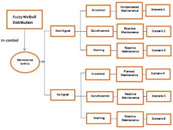
Initially, integrating model for Fuzzy Weibull Distribution economic model by EWMA Control Chart are carried out. As shown in Fig. 1, the framework of model integration illustrates six different scenarios, in which each scenario is further elaborated as following.

 _{In Scenario 1, the process starts at an “in-control” state and inspections begin after}

h

_{hours of} monitoring to check whether the process has shifted from an “in-control” to an “out-of-control” state. When the process needs maintenance before the scheduled time, an alert signal will appear in the control chart. But if the signal is false, the process will still be in-control. However, detection of false signal consumes time and cost, Compensatory Maintenance will be carried out.

(4)

 In Scenario 3, the process starts at an “in-control” state and inspections begin after

h

hours of monitoring to check whether the process has shifted from an “in-control” to a “warning limit” state. There will be an alert signal in the control chart when maintenance should be performed before the scheduled time.

 In Scenarios 4 and 5, there is no signal in the control chart before the scheduled time so at the th

(

k



1)

sampling interval, appropriate maintenance is arranged. In Scenario 3, the process will always be “in-control” and Planned Maintenance is performed. However, if the process shifts to an of-control” state in Scenario 4, Reactive Maintenance will be active. This is because the “out-of-control” condition occurs before the scheduled time, and additional time and expense will be incurred to identify and solve the equipment problem.

 In Scenario 6, the process starts at an “in-control” state and no signal occurs in the control chart before the scheduled time. Subsequently, at the th

[image:4.595.118.468.285.547.2]

(

k



1)

sampling interval, appropriate maintenance should be arranged. Moreover, in Scenario 6, the process is always “in-control” so Planned Maintenance will be performed.

Fig. 1. Integrated model scenarios.

2.1. Nomenclature Cycle Time

E T

[ ]

0

T

: The expected time searching for a false alarm

P

T

: The expected time to identify maintenance requirement and to perform a Planned Maintenance

A

T

: The expected time to determine occurrence of assignable causes

R

T

: The expected time to identify maintenance requirement and to perform a Reactive Maintenance

C

T

: The expected time to perform a Compensatory Maintenance



: The mean elapse time from the last sample before the assignable cause to the occurrence of the assignable cause

I

(5)

O

ARL

: The average run length during out-of-control period

E

: The expected time to sample and chart one item

(

,

)

P R C A

   

: The indicator variable (If it equals 1 production continuous during Planned Maintenance (Reactive Maintenance, Compensatory Maintenance, validate assignable cause) or 0 otherwise)

I i

P : The probability that run length of control chart equals i during in-control period

O i

P : The probability that run length of control chart equals

i

during out-of-control period

w i

P : The probability that run length of control chart equals

i

during warning period

d

: The interval between sampling

r

: The exponential weight constant Cycle Cost

E C

[ ]

I

C

: The cost of quality loss per unit time (the process is in an in-control state) often estimated by a Taguchi Loss function

O

C

: The cost of quality loss per unit time (the process is in an out-of-control state) often estimated by a Taguchi Loss function

P

C

: The cost of performing Planned Maintenance

R

C

: The cost of performing Reactive Maintenance

C

: The cost of performing Compensatory Maintenance

F

C

: The fixed cost of sampling

V

C

: The variable cost of sampling

f

C : The cost to investigate a false alarm Optimal Variable

h

: The interval between sampling. ( *

h

for optimal)

n

: The sampling size. ( *

n

for optimal)

k

: The number of sample taken before Planned Maintenance. ( *

k

for optimal)

L

: The width control limit in unit of standard deviation. ( *

L

for optimal)

w

: The width of warning control limit in units of standard deviation. ( *

w

for optimal)



: The number of subintervals between two consecutive sampling times. (



*

for optimal)

2.2. Basic Concept of Fuzzy Set and Some Definitions

In this section, the basic concepts and definition used in the study will be discussed. For classical set theory, it is defined that an element

x

in a universe U may or may not be a membership of some crisp set

A

. And this binary membership can be explained using the indicator function as below.

1 if x

A

( )

0 if x

A

x



_{ }









(1)

Zadeh [33] further described the notation of binary membership to cover various degree of

x

membership on the real continuous interval

[0,1]

, and defined the fuzzy set

A

by the membership function

( ) [0,1]

A x



 . Given



_A( )x be the degree of membership of element in fuzzy set







, _A( ) ;



(6)

2.3. Fuzzy Weibull Distribution

From the report of Karpisek et al. [27], the values of a fuzzy random variable

T

can be described by the fuzzy number t 



[0, ),



_t



and t





t

where

t

is the observed value of a crisp random variable T. Given that



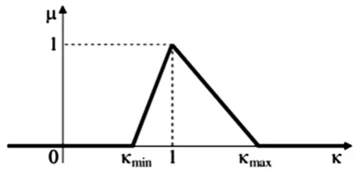
is a vagueness coefficient. This results in a triangular fuzzy number







[0, ),



_



with the main value





1

(Fig. 2). Then a membership function can be written by

min

min min

max

max max

, [ ,1] 1

( ) , [1, ] 1

0 , otherwise



 

_



 

 





 _

  

 

_{ } 

   

(2)

[image:6.595.176.430.353.478.2]

where

0 



min

 

1 

max, and boundary values



min

,



max are determined by an expert’s estimate.

Fig. 2. Triangular fuzzy number of

 

_

( )

.

If a random variableThas a crisp Weibull probability distribution

W v

( , )



, the corresponding fuzzy random variable Twith the Fuzzy Weibull probability distribution

W v

( , )



will have the following fuzzy characteristics. For

  

t

[0, )

, the fuzzy distribution cumulative function will be

[ ]

( ) 1 t

F t  e  where



, ,

v t



0

,





0.

(3) And, the fuzzy distribution cumulative function in the form of





cut

is

max max

min min [[(1 ) ] ]

[[(1 ) ] ]

( ) [ ( ), ( )]

1 , 1 , [0,1].

L U

t t

F t F t F t

e  e 

  

   

      

_

  



 

_   _   (4)

Then, the Process Failure Mechanism that follows a Fuzzy Weibull distribution is considered. Denote:

   

1   ( )

v

v v t

(7)

Subsequently, the fuzzy probability density function in the form of





cut

can be described as follows:









 

  









 

   max max min min

1 (1 ) min min

1 (1 ) max max

( ) [ ( ), ( )]

(1 )

, [0,1].

, (1 )

v

L U

v v t

f t f t f t

v t e

                                            (6)

2.4. Centroid Method

This approach, also called center of area or center of gravity, is one of most popular and effective defuzzification methods (Sugeno [34] and Lee [35]); it is expressed in the term of algebraic function.

*

( )

C C

z zdz

z

z dz







(7)

2.5. Integrated Model Scenarios

In this study, the integrated systems approach for process control and maintenance model proposed by Charongrattanasakul and Pongpullponsak [14] will be further adapted by combining with Fuzzy Weibull distribution. Using the Lorenzen and Vance model and cost function, the expected cycle time and cycle cost for each of the six scenarios is described as below:

Scenario 1:

1 1 1

0 0

1 1

[

]

[

]

, [

]

(1

( ))

,

(1

( ))

,

L U

k k

I I

i L C i U C

i i

E T S

h

ip

F

ih

T

h

ip

F

ih

T

      





 









_









_







(8)

1 1 1

0 0

[ ] [ ] , [ ]

[ (1 ( )) ] ( ) (1 ( ))

. , [ (1 ( )) ] ( ) (1 ( ))

L U

k k

I I

I i L C C F V i L f C

i i

k k

I I

I i U C C F V i U f C

i i

E C S E C S E C S

C h ip F ih T C nC ip F ih C C

      



          _ _ _ _ _ _ _                   



(9) Scenario 2:

2 2 2

0

[ ] [ ] , [ ] ( ( 1) )

, , ( ( 1) )

L U

kh

L O L A R

kh

U O U A R

E T S E T S E T S

tf t k h dt hARL nE T T

(8)









2 2 2

0

2

0

2

[ ] [ ] , [ ] ( ( 1) ) 1

[ ] ( ) , ( ( 1) )

1

[ ] ( )

L U

kh

I L O O A A R R

L F V R

kh

I U O O A A R R

U F V R

E C S E C S E C S

C tf t k h dt C hARL nE T T

E T S C nC C

h

E T S C nC C

h       









                                 _ _  _ _ __ _{ } _ _  _ _       



.        (11) Scenario 3:

3 3 3

1 0

[ ] [ ] , [ ] ( ( 1) ) (1 )

, , ( ( 1) ) (1 )

L U

kh

L L o O L A R

kh

U U o O U A R

E T S E T S E T S

tf t k h dt s T hARL nE T T

        













                                   



(12)

3 3 3

0 3 2 1 0 0 0 [ ] [ ] , [ ] ( ( 1) )

1

[ ]( ) (1 ) ( )

, ( ( 1) )

L U

kh

I L O O A A R R

F V f R

i i

kh

I U O O A A R R

E C S E C S E C S

E T S C nC C s C

d h id

      













                     _ _                      







3 2 1 0 0 . 1 [ ]( ) (1 ) ( )

F V f R

i i

E T S C nC C s C

d h id

 













                   _ _   _ _             _{ } _    



 (13) Scenario 4:





4 4 4

[

]

[

]

,

[

]

(

1)

, (

1)

,

L U

P P

E T S

k

h

T

k

h

T



 



 









(14)









4 4 4

[ ] [ ] , [ ]

( 1) ( )

. , ( 1) ( )

L U

I P P F V P

E C S E C S E C S

C k h T k C nC C

(9)

Scenario 5:





5 5 5

[

]

[

]

, [

]

(

1)

, (

1)

,

L U

R R

E T S

k

h

T

k

h

T



 



 









(16)

5 5 5

0 0

[ ] [ ] , [ ]

( ( 1) ) ( 1) ( ( 1) ) ( )

, ( ( 1) ) ( 1) ( ( 1) ) ( )

L U

kh kh

I L O L R R F V R

kh kh

I U O U R R F V R

E C S E C S E C S

C tf t k h dt C k h tf t k h dt T k C nC C

                                                            



.         _ (17) Scenario 6:





6 6 6

[

]

[

]

, [

]

(

1)

, (

1)

,

L U

R R

E T S

k

h T

k

h T



 



 









(18)

6 6 6

0 0

[ ] [ ] , [ ]

( ( 1) ) ( 1) ( ( 1) ) ( )

, ( ( 1) ) ( 1) ( ( 1) ) ( )

L U

kh kh

I L O L R R F V R

kh kh

I U O U R R F V R

E C S E C S E C S

C tf t k h dt C k h tf t k h dt T k C nC C

                                                            



.         _ (19)

2.6. Fuzzy Expected Hourly Cost E H[ ]_

The model can be considered as a renewal-reward process; hence, the fuzzy expected cost per hour

[ ]

E H _ can be expressed as

[ ]

[

]

,

[ ]

E C

E H

E T

  



(20) where

1 1 2 2 3 3 4 4

5 5 6 6

[ ]

[

]

( )

[

]

(

)

[

]

(

)

[

]

(

)

[

]

(

)

[

]

(

),

E T

E T S

P S

E T S

P S

E T S

P S

E T S

P S

E T S

P S

E T S

P S

        

   





(21)

and

1 1 2 2 3 3 4 4

5 5 6 6

[ ]

[

]

( )

[

]

(

)

[

]

(

)

[

]

(

)

[

]

(

)

[

]

(

).

E C

E C S

P S

E C S

P S

E C S

P S

E C S

P S

E C S

P S

E C S

P S

        

   





(22)

Fuzzy Probability of scenario 1:

1

1 1

( )

(1

( )) ,

(1

( )) ,

k k

I I

i L i U

i i

P S

_

P

F

_

ih

P

F

_

ih

 







_



_







(23)

(10)

1 1

1 1 1

2 ₁ ₁

1 1 1

[

( )

(

1) ](1

)

(

)

,

[

( )

(

1) ](1

)

k i k i

I O

L L j l

i j l

k i k i

I O

U U j l

i j l

F

ih

F

i

h

P

P S

F

ih

F

i

h

P

                



_





























 



 

(24)

1 1

1 1 1

3 ₁ ₁

1 1 1

[

( )

(

1) ](1

)

(

)

,

[

( )

(

1) ](1

)

k i k i

I w

L L j l

i j l

k i k i

I w

U U j l

i j l

F

ih

F

i

h

P

P S

F

ih

F

i

h

P

                



_





























 



 

(25)

1 4

1

(1 ( )) (1 ( ))

( ) ,

, (1 ( )) (1 ( ))

k I

L i L

i k

I

U i U

i

F kh P F ih

P S

F kh P F ih

        _ _ _               



(26)

1 1

1 1 1

5 ₁ ₁

1 1 1

(

)

[

( )

(

1) ](1

)

(

)

,

(

)

[

( )

(

1) ](1

)

k i k i

I O

L L L j l

i j l

k i k i

I O

U U U j l

i j l

F

kh

F

ih

F

i

h

P

P S

F

kh

F

ih

F

i

h

P

                  



_





























 



 

(27)

1 1

1 1 1

6 ₁ ₁

1 1 1

(

)

[

( )

(

1) ](1

)

(

)

.

,

(

)

[

( )

(

1) ](1

)

k i k i

I w

L L L j l

i j l

k i k i

I w

U U U j l

i j l

F

kh

F

ih

F

i

h

P

P S

F

kh

F

ih

F

i

h

P

                  



_





























 



 

(28)

As above, the integrated model for economic EWMA chart is obtained. The next step is to determine the optimal values of the six test variables

( , , , , , )

n h k L w



, in which consequently, the expected total cost per hour in Eq. (20) can be minimized.

According to examination of the components in Eq. (21) and Eq. (22), it can be seen that determining economically optimal values of the six test variables for the EWMA chart is not straightforward. To illustrate the nature of the solutions obtained from economic design of EWMA chart, a particular numerical example is provided.

2.7. Integrated Model of EWMA Control Chart by Genetic Algorithm

The solution procedure is carried out using genetic algorithms (GA) with MATLAB software to calculate the optimal values of * * * * *

,

n h

k

L w

_and



*that minimize



* *



[ ] ,_L [ ]_U

(11)

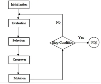
The GA, a random optimization search tool, has been developed on the basis of natural genetics. One of famous GA models in science and engineering have been introduced and investigated by Holland [36]. The technique uses the concept of Darwinian evolution in solving problems, where the solution of a problem is called a ‘‘chromosome’’. Theoretically, a chromosome contains many genes, in which each gene represents one feature or character. Among numerical optimization methods, such as neural network, gradient-based search, etc., the GA exerts several advantages in the following aspects:

1. The GA operates using the fitness function values and the stochastic method (not deterministic rule) in directing the finding approach for optimal solution. Accordingly, the GA can be applied to optimize problems in various fields.

2. The GA has mutation and crossover properties so it can determine a global optimum and help to avoid trapping in the local optimum.

3. The GA yields a number of possible solutions (or chromosomes) at one operation round. This increases a chance to obtain the global optimal solution efficiently. For this reason, this technique can be used for solving not only combinatorial optimization problems, but also in many areas (Jensen [37], Chou and Chen [38], Chou, Wu and Chen [39]).

[image:11.595.125.456.306.580.2]

The solution procedure for our example using the GA by MATLAB is briefly described as illustrating in Fig. 3.

Fig. 3. The solution procedure using genetic algorithm.

3. Numerical Example

In this section, the effect of model parameters on the solution of economic design of the EWMA chart is investigated. To do this, the GA is applied in searching the optimal solution of the economic design in each

 

0,1



 after substituting the fixed parameters (as shown in Table 1.) into Eq. (20). The obtained optimal six variables



* * * * * *



, , , , ,

n h k L w



and * *

[ ] ,_L [ ]_U

E H E H

 

(12)

[image:12.595.67.530.104.181.2]

Table 1. Fix Parameter on economic design.

I

C



10

C



2000

T

P



0.8

T

C



0.6

r



0.1

O

C



200

C

F



20

T

R



1



1





2





3



1

E



0.1

P

C



3000

C

V



0.1

T

A



0.3



min



0.5





0.05

R

[image:12.595.62.527.225.426.2]

C



4000 Cf 200

T

0



0.2



max



1.5

Table 2. The optimal six variables and total hourly cost in each





 

0,1 (Lower).

cut





*

n

h

* *

L

k

*

w

*



* E H*[ ]L

0 



_4.961 _5.107 _2.989 _21.001 _2.163 _8.036 _209.846

0.1 



_4.936 _9.817 _2.974 _22.076 _2.008 _9.209 _210.594

0.2 



_4.958 _8.459 _2.996 _22.145 _2.209 _7.108 _210.618

0.3 



_4.997 _5.482 _2.973 _20.158 _2.023 _9.098 _211.731

0.4 



_4.955 _9.219 _2.992 _22.136 _2.003 _9.048 _212.101

0.5 



_4.931 _5.482 _2.997 _22.048 _2.191 _9.924 _212.542

0.6 



_4.961 _7.279 _2.957 _21.064 _2.023 _9.723 _214.085

0.7 



_4.997 _5.602 ₃ _21.043 _2.201 _7.291 _214.138

0.8 



_4.994 _5.189 _2.996 _21.064 _2.421 _8.245 _214.284

0.9 



_4.941 _5.013 _2.999 _20.003 _2.205 _8.453 _216.134

1

[image:12.595.66.527.468.671.2]





_4.732 _9.571 _2.999 _25.264 _2.481 _9.975 _216.259

Table 3. The optimal six variables and total hourly cost in each





 

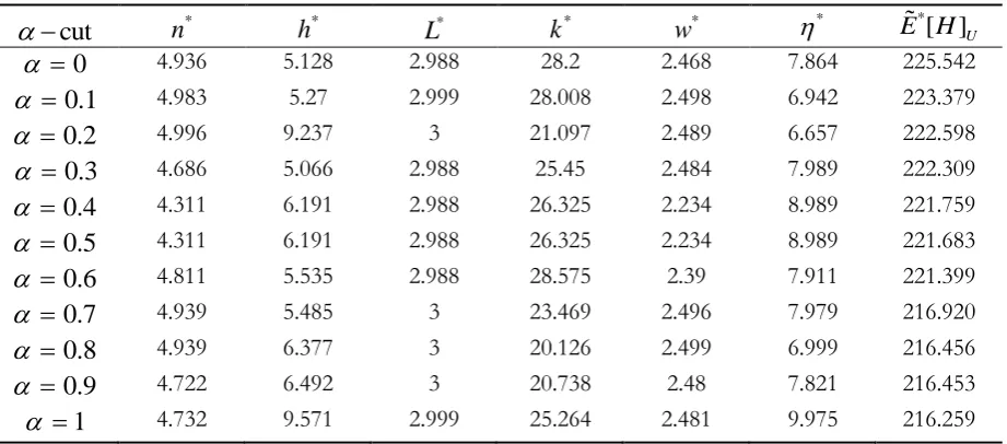
0,1 (Upper).

cut





*

n

h

* *

L

k

*

w

*



* E H*[ ]_U

0 



4.936 5.128 2.988 28.2 2.468 7.864 225.542

0.1 



4.983 5.27 2.999 28.008 2.498 6.942 223.379

0.2 



4.996 9.237 3 21.097 2.489 6.657 222.598

0.3 



4.686 5.066 2.988 25.45 2.484 7.989 222.309

0.4 



4.311 6.191 2.988 26.325 2.234 8.989 221.759

0.5 



4.311 6.191 2.988 26.325 2.234 8.989 221.683

0.6 



4.811 5.535 2.988 28.575 2.39 7.911 221.399

0.7 



4.939 5.485 3 23.469 2.496 7.979 216.920

0.8 



4.939 6.377 3 20.126 2.499 6.999 216.456

0.9 



4.722 6.492 3 20.738 2.48 7.821 216.453

1 



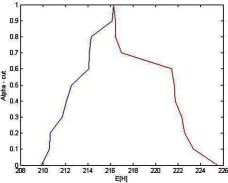
4.732 9.571 2.999 25.264 2.481 9.975 216.259

(13)

[image:13.595.177.409.82.268.2]

Fig. 4. Membership functions of total hourly cost.

As shown in Fig. 4, the optimal values of the policy variables, whose minimize *

[

]

E H

_{, are}

n

*_=4.939, *

h

=5.485, *

L

= 3, *

k

= 23.469, *

w

= 2.496,



*

= 7.979, and the corresponding hourly cost is *

[

]

E H

= 216.920.

4. Conclusion and Discussion

Generally, development of integrated model considers advantages of two traditions but separately uses manufacturing process control tools, which are covering statistical process control and maintenance management. In this research, an integrated economic model has been developed by combining Fuzzy Weibull distribution into EWMA control chart. To minimize the fuzzy expected total cost per hour

( [E H] , [L E H] )U , the obtained model is used to determine the values of six tested variables of the chart

including the sampling interval

( )

h

, the sample size

( )

n

, the number of samples taken before Planned Maintenance

( )

k

, the width of control limit in units of standard deviation

( )

L

, the width of warning control limit in units of standard deviation

( )

w

and the number of subintervals between two consecutive sampling times

( )



. The fuzzy expected total cost per hour is then transformed from fuzzy data to crisp data by the centroid method. Additionally, the cost function is analyzed on the basis of the cost model described in Linderman and Kathleen [15]. Finally, using Genetic Algorithm approach an illustrative example is demonstrated to search for the solution of economic design.

Table 4. A comparison of optimal total hourly cost for six models between crisp data and fuzzy data under condition of using the same variable.

Six models with crisp data [14] _{(the proposed model in this study)}Six models with fuzzy data Variable Integrated Model Variable Integrated Model

*

n

4.939

n

* 4.939

*

h

5.485

h

* 5.485

*

k

23.469

k

* 23.469

*

w

2.496

w

* 2.496

*



7.979



* _7.979

*

L

3

L

* 3

*

[

]

E H

219.624 *

[

]

[image:13.595.78.522.615.774.2]

(14)

From Table 4, a comparison between two methods under given assumption (using the same variable) is investigated. The optimal total hourly cost for six models with crisp data is 219.624 [14] whereas the optimal total hourly cost for six models with fuzzy data is 216.921 which is decreasing from the six models with crisp data for 2.703. From the results, it can conclude that the optimal total hourly cost for six models with fuzzy data depends on variables or types of products.

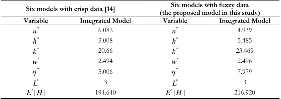
Table 5 shows a comparison of optimal total hourly cost for six models between crisp data and fuzzy data. It can be seen that using the six scenarios model [14], the optimal sample size *

( )

n

and the optimal interval between samples *

( )

h

are equal to 6.082 and 3.008, respectively whereas using the proposed model, the optimal sample size *

( )

n

and the optimal interval between samples *

( )

h

are 4.939 and 5.485, respectively. Clearly, the optimal sample size *

n

obtained from this study is lower than that of the six scenarios model [14] for 1.143, and the optimal interval between samples *

[image:14.595.74.522.339.497.2]

h

obtained from this study is increased from the six scenarios model [14] for 2.477. It is because this research uses warning limit, in which the sample frequency will be increased when the product warning in the system is alarm. This causes product analysis more efficient, resulting in reducing of low quality products. However, the cost will be higher.

Table 5. A comparison of optimal total hourly cost for six models between crisp data and fuzzy data.

Six models with crisp data [14] _{(the proposed model in this study)}Six models with fuzzy data Variable Integrated Model Variable Integrated Model

*

n

6.082

n

* 4.939

*

h

3.008

h

* 5.485

*

k

20.66

k

* 23.469

*

w

2.494

w

* 2.496

*



5.006



* _7.979

*

L

3

L

* 3

*

[

]

E H

194.640

E H

*

[

]

216.920

In addition to the optimal interval between samples *

( )

h

, from Table 5 it is observed that by using the model in this study the optimal number of subintervals between two consecutive sampling times *

(



)

is higher than that of the six scenarios model [14]. The optimal number of subintervals between two consecutive sampling times *

(



)

from the six scenarios model [14] is 5.006 whilst the



*

values tested in this study is 7.979. It is also seen that the



*

values from this study is higher than that of the six scenarios model [14] for 2.973. One explanation is that the value of the number of subintervals between two consecutive sampling times is depended on the interval between samples. Thus if the sampling is too high, the value of the number of subintervals between two consecutive sampling times will be high too.

Finally, as shown in Table 5 the hourly cost *

[ ]

E H

 

 from the six scenarios model [14] is 194.640.

When using the proposed model, the hourly cost *

[ ]

E H

 

  equals to 216.920, which is higher than the

value of the six scenarios model [14] for 22.28. This is because the addition of the fuzzy concept in the model increases ability of detection of defective products and frequency of sampling, thereby increasing product investigation and more detected defective products. This leads into increased repairing and maintenance of machines; thus the hourly cost *

[ ]

E H

 

 is higher.

(15)

use of the new fuzzy Weibull control, the more expenses in maintenance, but the lower lots rejection and perhaps lower in consumers' risk. The last one is better.

Acknowledgments

This work is supported by the Centre of Excellence in Mathematics (CEM) and the Faculty of Science, KMUTT.

References

[1] M. A. Girshick and H. Rubin, “A Bayes approach to a quality control model,” Ann. Math. Statist,vol. 23, pp. 114–125, 1952.

[2] A. J. Duncan, “The economic design of

X

chart used to maintain current control of a process,” Journal of the American Statistical Association, vol. 51, 1956.

[3] T. C. Lorenzen and L. C.Vance, “The economic design of control charts: A unified approach,” Technometrics, vol. 28, pp. 3–10, 1986.

[4] S. M. Alexander, J. S. Dillman, M. A. Usher, and B. Damodaran, “Economic design of control charts using the Taguchi loss function,” Computers and Industrial Engineering, vol. 28, pp. 671–679, 1995. [5] M. A. Rahim and P. K. Banerjee, “A generalized model for the economic design of control chart for

production systems with increasing failure rate and early replacement,” Navel Research Logistics, vol. 40, pp. 787–809, 1993.

[6] C. R. Cassady, R. O. Bowden, and E. A. Pohl, “Combining preventive maintenance and statistical process control: A preliminary investigation,” IIE Transactions, vol. 32, pp. 471–478, 2000.

[7] T. G. Yeung, C. R. Cassady, and K. Schneider, “Simultaneous optimization of control charts and age-based preventive maintenance policies under an economic objective,” IIE Transactions, vol. 40, pp. 147-159, 2008.

[8] M. Ben-Daya and M. A. Rahim, “Effects of maintenance on economic design of an control chart,” European Journal of Operation Research, vol. 120, pp. 131–143, 2000.

[9] S. Panagiotidou and G. Nenes, “An economically designed, integrated quality and maintenance model using an adaptive Shewhart chart,” Reliability Engineering and System Safety, vol. 94, pp.732–741, 2009. [10] J. Wu and V. Makis, “Economic and economic-statistical design of a chi-square chart for CBM,”

European Journal of Operational Research, vol. 188, pp. 516–529, 2008.

[11] D. A. Serel and H. Moskowitz, “Joint economic design of EWMA control charts for mean and variance,” European Journal of Operational Research, vol. 184, pp. 157–168, 2008.

[12] K. Linderman, K. E. McKone-Sweet, and J. C. Anderson, “An integrated systems approach to process control and maintenance,” European Journal of Operational Research, vol. 164, pp. 324–340, 2005.

[13] W.-H. Zhou and G.-L. Zhu, “Economic design of integrated model of control chart and maintenance,” Mathematical and Computer Modeling, vol. 47, pp. 1389–1395, 2010.

[14] P. Charongrattanasakul and A. Pongpullponsak, “Minimizing the cost of integrated systems approach to process control and maintenance model by EWMA control chart using genetic algorithm,” Expert Systems with Applications, vol. 38, pp. 5178–5186, 2011.

[15] S. O. Caballero Morales, “Economic statistical design of integrated X-bar-s control chart with preventive maintenance and general failure distribution,” PLoS ONE, vol. 8, pp. e59039, 2013.

[16] H. Yin, G. Zhang, H. Zhu, Y. Deng, and F. He, “Integrated model of statistical process control and maintenance based on the delayed monitoring,” Reliability Engineering and System Safety, vol. 133, pp. 323–333, 2015.

[17] B. Russell, “Vagueness,” Australasian J Psychol Philos, vol. 1, pp. 84–92, 1923.

[18] L. A. Zadeh, “Outline of a new approach to the analysis of complex systems and decision processes,” IEEE Transactions on Systems, Man, Cybernet, vol. 3, pp. 28–44, 1973.

[19] W. A. Lodwick and K. D. Jamison, “Interval-valued probability in the analysis of problems containing a mixture of possibilistic, probabilistic and interval uncertainty,” Fuzzy Set Systems, vol. 159, pp. 2845– 2858, 2008.

[20] L. A. Zadeh, “From imprecise to granular probabilities,” Fuzzy Set Systems, vol. 154, pp. 370–374, 2005. [21] K. S. Park, “Fuzzy set theoretic interpretation of economic order quantity,” IEEE Transactions on

(16)

[22] S. C. Chang, “Fuzzy production inventory for fuzzy product quantity with triangular fuzzy number,” Fuzzy Sets and Systems, vol. 107, pp. 37-57, 1999.

[23] S. H. Chen and C. H. Hsieh, “Representation, ranking, distance, and similarity of L-R type fuzzy number and application,” Australian Journal of Intelligent Processing Systems, vol. 6, pp. 217-229, 2000. [24] C. H. Hsieh, “Optimization of fuzzy production inventory models,” Information Sciences, vol. 146, pp.

29-40, 2002.

[25] H. M. Lee and J. S. Yao, “Economic production quantity for fuzzy demand quantity and fuzzy production quantity,” European Journal of Operational Research, vol. 109, pp. 203-211, 1998.

[26] D. C. Lin and J. S. Yao, “Fuzzy economic production for production inventory,” Fuzzy Sets and Systems, vol. 111, pp. 465-495, 2000.

[27] Z. Karpisek, P. Stepanek and P. Jurak, “Weibull fuzzy probability distribution for reliability of concrete structures,” Engineering Mechanics, vol. 17, pp. 363–372, 2010.

[28] E. Baloui Jamkhaneh, “An evaluation of the systems reliability using fuzzy lifetime distribution,” Journal of Applied Mathematics Islamic Azad University of Lahijan, vol. 7, pp. 73-80, 2011.

[29] E. Baloui Jamkhaneh, “Reliability estimation under the fuzzy environments,” The Journal of Mathematics and Computer Science, vol. 5, pp. 28-39, 2012.

[30] S. Rezvani, “A new method for ranking in perimeters of two generalized trapezoidal fuzzy numbers,” International Journal of Applied Operational Research, vol. 2, pp. 85-92, 2012.

[31] E. Baloui Jamkhaneh, “Analyzing system reliability using fuzzy weibull lifetime distribution,” International Journal of Applied Operational Research, vol. 4, pp. 93-102, 2014.

[32] S. Sorooshian, “Fuzzy approach to statistical control charts,” Journal of Applied Mathematics, 2013. [33] L. A. Zadah, “Fuzzy sets,” Information Control, vol. 8, pp. 338-353, 1965.

[34] M. Sugeno, “An introductory survey of fuzzy control,” Inf. Sci., vol. 36, pp. 59–83, 1985.

[35] C. Lee, “Fuzzy logic in control systems: Fuzzy logic controller Parts I and II,” IEEE Transactions on Systems, Man, Cybernetics, vol. 20, pp. 404–435, 1990.

[36] J. H. Holland, Adaptation in Natural and Artificial Systems. Ann Arbor: Univ. Michigan Press, 1975. [37] M. T. Jensen, “Generating robust and flexible job shop schedules using genetic algorithm,” IEEE

Transactions on Evolutionary Computation, vol. 7, pp. 275– 288, 2003.

[38] C. Y. Chou and C. H. Chen, “Economic design of variable sampling intervals control charts using genetic algorithms,” Expert Systems with Applications, vol. 30, pp. 233–242, 2006.