This is the accepted version of the following paper:
Christopher D. Lloyd (2015) Local cost surface models of distance
decay for the analysis of gridded population data. Journal of the Royal
Statistical Society, Series A, 178: 125–146.
Local cost surface models of distance decay for the analysis of
gridded population data
Summary
This paper evaluates a number of proposed improvements to the analysis of gridded population data, using as a case study the religious segregation observed in gridded population data from Northern Ireland. First, the use of cost surfaces rather than simple Euclidean (straight line) distances to represent the interactions between gridded geographic areas. Second, a method for creating gridded cost surfaces that takes account of vector features (such as roads and physical obstructions). Third, the limitation of cost surfaces to a tightly defined ‘local’ set of areas, with a view to significantly reduce computational overheads without adversely impacting the accuracy of subsequent results. The results suggest that all three improvements have merit. The paper further explores the impact of using log ratios rather than percentages (minimal) and of local rather than global measures of segregation (which allows for considerably greater insight into population characteristics). Although the case study and results apply specifically to gridded population data, the results of the paper have wider implications for the analysis of any type of zonal data.
1. Introduction
This paper examines a number of key issues relating to the analysis of spatially aggregated data, using as a case study the religious segregation observed in gridded population data from Northern Ireland. First and foremost, this paper explores the possibilities offered by using cost surfaces rather simple Euclidean (straight line) distances to represent the interactions between gridded geographic areas. The distance between people (or, at least, between the areas they live in) is often taken as a proxy for interactions between them. In spatial analyses involving spatial regression or spatial autocorrelation of numerical population data it is the norm to adopt the convenient fiction of modelling these interactions as a simple function of Euclidean distance. Yet, as Cliff and Ord (2009) note, these simple functions of distance ignore anisotropy (directional variation) and assume spatial homogeneity. In reality, interactions between people are a function of multiple complex factors. These may include distance, cultural or economic difference, mode of interaction (residential, workplace, leisure,…) and other physical and perceptual obstructions. For this reason, in some contexts, such as spatial interaction modelling using flow data (for example, on commuting or migration), time or road distance-based measures are commonly applied.
Cost distance approaches may help to overcome the limitations of simple functions of distance. Costs are generally expressed as travel time or the ‘effort’ associated with crossing a cell rather than financial cost, and cost distances can be computed such that, for example, speed of travel along particular roads is accounted for and obstructions such as water bodies can be included. For example, cost distances (based on a friction surface in a raster (data values on a regular grid) context) have been used by Greenberg et al. (2011) to determine weights for spatial interpolation of water temperature in a complex deltaic river system, where straight line distances between samples are not meaningful. For a more general discussion of notions of distance other than simple Euclidean distance see Lowe and Moryadas (1975) and Gatrell (1983).
this ‘distance decay’ does not generally follow a simple linear relationship with the cumulative cost of the distance between areas. For this reason a wide range of distance decay functions have been considered, such as the inverse distance and Gaussian (see, for example, Lloyd 2011). It has also widely been recognised that the applicable distance decay function may well vary from place to place, leading to functions with locally varying parameters, such as the bi-square adaptive kernel (Fotheringham et al., 2002). Cliff and Ord (2009) further note that the use of weight schemes (used in measuring spatial autocorrelation, for example) which are not based on adjacency of areas is still under-developed; a shortcoming that this paper addresses. Getis and Aldstadt (2004), in a study concerned with deriving local weights matrices, provide a useful summary of alternative forms of geographical weighting (distance decay) functions.
Not only is the nature of the distance decay function debated; so is the range, or size of neighbourhood, over which it should be operated. It is a given that the larger the neighbourhood considered, the more interactions that will be identified. However, there are computational and empirical reasons for choosing to limit neighbourhood size. From an empirical perspective, the vast majority of interactions take place with between entities (people) in spatially proximate areas. And from a computational perspective, there are major gains to be had from reducing the size of the problem set. Thus, using only some subset of the data in the calculation of each local statistic reflects the predominance of interactions over short distances and, compared to measuring distances and computing geographical weights for all observations, reduces computational effort.
Jointly, the combination of distance decay function and neighbourhood size defines a ‘weighting function’ which can be used to weight the interactions (distances) between the population in a given focal cell and the wider population. A weight of zero may be assigned to all interactions outside of the neighbourhood (an alternative approach is to weight all observations in the data set, but with negligible weights beyond a certain distance), whilst the weight assigned to interactions within the neighbourhood is determined by the distance decay function chosen.
A second key contribution of this paper is the introduction of a methodology for creating gridded cost surfaces that take account of vector features (such as roads and physical obstructions). Most applications of cost surfaces are based on friction surfaces derived directly from raster data sets, an example being maps of terrain slopes. An alternative approach, as employed here, is to construct a friction surface for input to cost surface analysis by rasterising vector features representing roads and also impediments to movement such as, in the following case study, peace walls (physical structures which divide different ‘religious’ communities in so-called ‘interface’ areas of Northern Ireland). Further, cost surfaces are generally computed from one cell to all other cells. Here, the concern is to derive a separate cost surface for each cell which represents the least cost from the cell to its neighbours. Computing costs only to some subset of the data (e.g., the closest cells) is computationally much easier than computing costs from each cell to all other cells in the data set.
computation time. Such an approach has potentially wide applicability in any context where spatial variation in gridded data is of interest.
Spatial autocorrelation is usually measured on a global basis – one measure is obtained which summarises clustering across the whole study area. Many spatial properties, including population groups, tend to cluster in some regions, but not others. Thus, to characterise these region-specific clusters, a local measure of spatial autocorrelation is needed. In this paper, different weighting schemes are applied for measurement of spatial autocorrelation both globally and locally with, in the latter case, a measure for each zone (here, 100m grid cell) in the study area.
Analysis of population variables, such as those contained in the religion dataset used in the case study presented here, is often based on percentages or proportions. Such data are termed compositional data and the sum of the parts is 100 (for percentages) and 1 (proportions); data of this type should not be analysed using standard statistical methods. Reasons for this include the potential for prediction of negative values when using regression with compositional data, the possibility of spurious correlations being induced between components of a composition because the data are closed (i.e., possible values range from 0 to 1 or 0 to 100), with a bias toward negative correlations, and subcompositional incoherence. As an example of the latter, it has been demonstrated that the covariance (and thus correlation coefficient) between variables can change markedly and with no apparent pattern, as parts of an original five-part composition are removed to form new four-part or three-part compositions (Aitchison, 1986). It has also been argued that univariate statistical methods are not appropriate for the direct analysis of raw compositional data (Filzmoser et al., 2009). Another concern of this paper, therefore, is to compare results derived using a sound statistical approach (log ratios) with results based on the common approach – use of untransformed percentages. For a discussion of alternative forms of log ratios and the justification for their use in place of percentages see Aitchison (1986), Filzmoser et al. (2009) and Lloyd et al. (2012).
Thus, the case study presented in this paper assesses the impact on results of using different (i) variable definitions (percentages and log ratios), (ii) distance metrics (Euclidean and cost distances), (iii) distance decay functions, (iv) neighbourhood sizes (with iii and iv combining to make a weighting scheme), and (v) global and local measures of spatial autocorrelation. Each of these issues is discussed in depth below and their importance is illustrated systematically through the case study. While these issues are explored through an analysis of the spatial autocorrelation amongst the religious communities of Belfast, the principles considered are applicable in any analysis of gridded spatial data, and, by extension, to any other less regular geography.
2. Case study
The data
that the changes in the percentage shares are of widespread interest in the region. In the present case study, Belfast Urban Area (BUA) provides the focus.
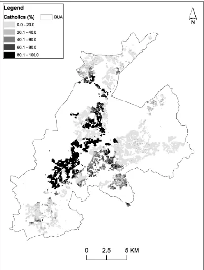
The case study makes use of counts of persons in BUA by community background for 100m grid squares, released as one of the outputs from the 2001 Census of Population (see Shuttleworth and Lloyd 2009, for more details on the grid square resource). For grid cells with less than 25 persons and/or eight households, counts are restricted to total persons, total males, total females and total households. The full set of counts, which include those for community background, are provided for cells only where those thresholds are exceeded. The imputation of non-responding individuals and small cell adjustment, used to prevent disclosure of information about individuals, have an impact on the counts used as the basis of the analysis, although the results are believed to be robust since the impact of small cell adjustment on the spatial structure of the percentages (and log ratios) is minor. Figure 1 shows the percentage of Catholics by community background for 100m cells in BUA. The 100m data for 2001 indicate that some 39.5% of the population of BUA were Catholic by community background, 56% were Protestant (or Other Christian) and 4.5% had a background associated with other religions or no religion.
FIGURE 1 ABOUT HERE
Measuring segregation
This paper presents one example of the use of Euclidean and cost distance measures for determining weights locally, and the particular focus is on the measurement of clustering of population groups. Such analyses have links to studies of residential segregation, which are concerned with the distribution of population subgroups and with interactions between these subgroups. There is a large body of research on the measurement of residential segregation which presents and applies measures of different dimensions of segregation (see Massey and Denton, 1988). Most measures are aspatial and are based on counts or proportions within zones; in these cases, interactions between zones are not taken into account. Poole and Doherty (1996) provide a study of segregation in Northern Ireland, while a more recent analysis is presented by Shuttleworth and Lloyd (2009), who explore changes in segregation between 1971 and 2001. In both of these publications, standard aspatial measures of segregation, such as the index of dissimilarity (D), are utilised. In another study concerned with Northern Ireland, Lloyd (2012) explores the spatial scale of variation in the population by religion.
The focus of this paper is on the measurement of clustering in the Catholic population which arises in the context that there are spatially distinct concentrations of Catholics and Protestants in some areas within the BUA. The value of D for Catholics as against Protestants and Other Christians in BUA in 2001 was 0.757 (excluding others from the calculations), suggesting a large degree of unevenness in the population (that is, the proportional share of the two groups varies markedly across the zones). Some 68% of Catholics lived in 100m cells which had 75% Catholics or more, while some 76% of Protestants lived in 100m cells which had 75% Protestants or more; in both cases percentages were computed from the total population.
Log ratios and Percentages
However, given small cell adjustment (see Williamson 2007) and non-responding we cannot be sure that there really are no members of the ‘other’ group (i.e., Catholics in ‘Protestant areas’ or Protestants in ‘Catholic areas’ ). Therefore, log ratios were used given percentages computed with n1 1 and n2 1, where n1 is the number of Catholics and
2
n is the number of non Catholics; this strategy was also employed by Lloyd (2010a). Addition of other alternative constants (e.g., n1 0.5 and n2 0.5) suggests that results
obtained using the log ratios are robust. In short, log ratios (𝑧1) were derived as follows:
2
2
1
n n
N 100 / ) 1 ( 1
1 n N
y
)) 100 /(
ln( 1 1
1 y y
z
Log ratios provide the main focus in the analysis, although raw percentages are used for comparative purposes.
3. Deriving the friction surface
The first stage of a cost surface analysis, used here to determine weights for spatial autocorrelation analysis, is the construction of a friction surface. The friction surface indicates the cost associated with crossing each given cell, while the cost surface derived from it indicates the minimum accumulative cost distance from a focal cell to other cells. In the case study presented here, data on roads and peace walls are used to determine costs. Members of the two main communities in Northern Ireland are physically separated in some areas (mostly in Belfast) by peace walls. The first of these walls were constructed in 1969 with the intention of reducing conflict in ‘interface’ areas where predominantly Catholic neighbourhoods share boundaries with predominantly Protestant neighbourhoods. Peace walls are an obvious case of a physical barrier across which daily interactions may be limited; other barriers in this and other contexts may consist of, for example, major roads, railways, or parks (Noonan 2005).
each measurement location, although for a much smaller number of observations than in the present study.
The vector road data used in the present case study are from the OSNI® (Ordnance Survey Northern Ireland) road network dataset. Roads include Motorways, A Class, B Class, and C Class roads. In addition, the dataset includes footpaths and car parks, as well as Unclassified features (including private roads, alleyways and tracks); these other features were not used in this study. Travel speeds were estimated for the various classes of roads and, for non-road cells, walking. The road travel figures were based on approximate maximum permitted road speeds which were reduced to reflect congestion and other factors which inhibit travel, particularly in urban areas. Following research on pedestrian walking speeds outlined by Laxman et al. (2010), an approximate speed of just under 80m/minute was specified, rounded to the nearest kilometre below. The travel speeds specified were considered to represent an improvement over the assumption of equal travel speeds by foot or by road:
Speed Time to cross
100m (minutes)
Average walking speed 5km/hour 1.2
Average speed on minor urban roads (U roads) 20km/hour 0.3
Average speed on B roads and C roads 40km/hour 0.15
Average speed on Motorways and A roads 80km/hour 0.075
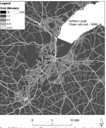
These figures are also expressed as the time taken to cross a 100m cell. The roads and peace wall vector data were combined and converted to a raster grid with a spatial resolution of 100 m – this corresponds to the gridded population data used in the case study (described below). Each raster cell received the cost associated with the overlapping vector line segment which had the longest length. For example, if a motorway segment and a minor urban road segment overlap a cell, then the longest of these two segments determines the cost attached to the cell. Here, movement across a road cell in a direction perpendicular to the road is the same as the cost of movement across the cell along the road. That is, moving across a road, rather than along it, presents an impediment to travel. While the approach could be refined, this is unlikely to have a major impact on results. Peace walls were assigned a nominal cost of 30 minutes. This figure was sufficient to ensure that movement around a peace wall by walking or any type of road was less costly than movement across the peace wall. Rasterisation of peace walls could lead to gaps through which modelled interactions are possible; in practice, the friction effect associated with peace walls was represented well.
FIGURE 2 ABOUT HERE
There is an assumption in the case study that the friction surface inputs (roads, peace walls) and Census data (for 2001) correspond to the same time period. Although there have been changes in the road network of Belfast in the more than ten years following 2001, these changes are unlikely to make a marked difference to modelled interactions on a local basis.
Cost distances for gridded data are computed from the friction surface with:
• Neighbours sharing an edge: average of costs in the neighbouring cells (e.g., 1.2 + 0.3 = 1.5/2 = 0.75)
• Neighbours sharing only a corner: average of costs in the neighbouring cells multiplied by 2 – here approximated by 1.4142 (e.g., (1.5+0.3)/2 = 1.5/2 = 0.75 × 1.4142 =
1.0607)
The cost surface procedure can be outlined as follows:
1. Compute the cost distances from the source (focal) cell to its neighbours. 2. Select the neighbouring cell with the smallest cost distance from the source cell. 3. Compute the cost distances from the newly selected cell to all of its neighbours and
activate these cells.
4. The activated cell with the smallest accumulative cost distance is selected and the cost distances to the neighbours of that cell are calculated. Every time a cell becomes accessible to a source cell through a different path it is reactivated and its accumulative cost must be recalculated as the new path may have a smaller accumulative cost. If it does not, then the accumulative cost value remains the same.
5. Repeat the above process until the smallest accumulative cost distances from the source cell to each possible destination cell have been computed
4. Computing local costs
Given the friction surface described above, least costs to the neighbouring cells are computed from each of the populated cells, and it is this locally-based cost surface construction which comprises the key original contribution of this paper. Costs could be computed from each populated cell to all other cells using the procedure outlined above, but this is prohibitively slow. It is also unnecessary given that weights, and thus costs, are only required in some local neighbourhood. For these reasons, costs were only computed up to some specified number of neighbouring cells. The approach taken here is to compute n least costs to populated neighbours of a populated focal cell. It is possible that some edge cells could be reached by less costly routes if n is increased, but this is likely to have only a minimal impact on results. A possible modification would be to compute, for example, least costs to 50 cells but retain only the 20 smallest costs. The costs were converted to weights in four ways, using the weighting schemes defined in Section 5. This local derivation of cost surfaces is a novel approach, and one which opens up the possibility of computing individual cost surfaces for multiple neighbourhoods with a low computational effort. This new approach has many potential applications, as considered later.
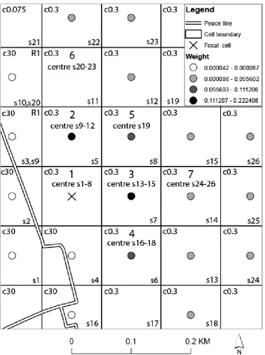
same if the cells were equally distant from the focal cell. Figure 3 also demonstrates how the least cost paths are derived in this example. The costs for moving between cells are computed as outlined in Section 3. The focal cell is labelled ‘1’ at centre top, and ‘centre s1-8’ indicates that it is the focal cell from which costs to cells labelled s1 to s8 are computed. The cost associated with each cell (its value in the friction surface) is indicated by the prefix ‘c’ – so c30 indicates a cost of 30 minutes. The algorithm scans around the focal cell from left to right and top to bottom, visiting the cell with ‘s1’ in its lower right corner, then the cell s2, onto s3, s4, s5, s6, s7, and finally s8. The (minimum) cost is stored at each stage. If there are several cells with the same smallest cost, the first minimum cost cell visited is selected. Here, this is the cell labelled ‘2’ at centre top. The cells around this cell are then scanned (that is, they are visited sequentially, in the same order as before), and costs determined for any cells which do not have a cost. If an existing accumulative cost associated with a cell is less through a cell which is newly assigned a cost, then a new accumulative cost is computed for that cell. This happens with the cell which includes s3,s9 at its base – it is cheaper to reach this cell in a path from the cell headed ‘1’ through to cell ‘2’, and then horizontally from cell ‘2’, than diagonally from cell ‘1’. The process continues until a predefined minimum of n least costs (for example, 20, including the source cell) is computed for populated cells. The value is a minimum because each new cell added to a path can introduce 0-5 neighbouring cells for which least costs need to be calculated. In practice, for a minimum of 20 least costs to populated cells (including the source cell), the number of least costs calculated ranged from 19 to 23 (since the focal cell is included, a minimum of less than 20 is possible). So, costs are computed to cells, including those which are unpopulated, until costs are available for at least n populated cells; the weights are then determined (using the functions defined in Section 5) from these costs and used to compute I (whether global or local).
FIGURE 3 ABOUT HERE
In this application, local costs can be computed for all locations as the limit of analysis is BUA and accumulative least costs near the borders of the area can be computed given values of the friction surface outside of the BUA. Were the analysis extended to the whole of Northern Ireland, then the friction surface would have to be determined in the border areas of the Republic of Ireland. The friction surface could be derived as for Northern Ireland, but the lack of equivalent gridded population data would mean that the n nearest populated cells would all be in Northern Ireland unless population surfaces on a 100m grid were derived from counts for irregular zones in the Republic of Ireland.
5. Alternative weighting schemes
illuminate the relative importance of choice of distance metric, distance decay function and neighbourhood type.
TABLE 1 ABOUT HERE
5.1 Queen Contiguity
In many applications, the proximity between locations i and j given by wij is set to 1 when locations i and j are neighbours, and 0 when they are not, with wij = 0 when i j . When zones sharing edges and vertices are included in the calculations, this is termed Queen case contiguity. Note that, by definition, the local neighbourhood for the Queen Contiguity weighting scheme simply comprises those cells immediately adjacent to the focal cell. The weights may be subsequently row-standardised – this refers to division of each weight in the weights matrix by the sum of its row. In words, the weights matrix comprises rows for each location i and columns for each location j, and the entries in each row can be standardised to sum to one. As an example, if zone i has four neighbours and each is given a weight of one, these are each standardised by division by four (the sum of the weights) and thus the weights each become 0.25.
5.2 Inverse Distance
Inverse distances are commonly employed in spatial interpolation contexts:
k ij ij d
w (1)
where dij is the distance between locations i and j.As above, the weights derived from
the function may be subsequently row-standardised by dividing each weight in the weights matrix by the sum of its row, such that the entries in each row will sum to one.
Reflecting common choices for the value of the exponent k, the inverse distance function is used to define three weighting schemes for this paper. The first uses k=1 (representing linear distance decay); the second and third use k= 2 (the so called ‘gravity’ model) (numbers 2, 3, and 4 in Table 1). The local neighbourhood is defined for the first two weighting schemes (k=1; k=2) as the n populated cells with least accumulative costs from the focal cell (‘nearest n’). For the third weighting scheme, also with k=2, the local neighbourhood is defined as all cells within a particular travel time (accumulative cost distance or ‘time limit’) of the focal cell. For the three inverse distance weighting schemes considered in this paper the weights of all cells outside of a defined local neighbourhood are set to zero.
The weights shown in Figure 3 are of row-standardised inverse square weights (i.e., k=2). In this case, the weights are standardised to sum to one and the function corresponds to a form of weighted average of the values in a particular locality (e.g., 20 nearest neighbours) (Anselin, 1995))
5.3 Gaussian Fixed Kernel
] ) / ( 5 . 0
exp[ ij 2
ij d
w (2)
Where, as before, dij is the distance between locations i and j, and is the bandwidth
which determines the size of the spatial kernel. For the purposes of this paper the local neighbourhood for this weighting scheme is defined as all grid cells within a fixed Euclidean distance of the focal cell. Importantly, the bandwidth (and thus the size of the kernel) is of the same size at all locations.
5.4 Bi-square Adaptive Kernel
In contrast, the final distance decay function considered is one in which the bandwidth and kernel size vary as a function of, for example, observation density or population number. In the case of observation density, the kernel is small in areas with large numbers of zones and large in areas with small numbers of zones. Thus, the kernel may be adapted to include (for example) the nearest ten observations to each location. The bi-square weighting function (see Fotheringham et al. 2002) defines one form of adaptive kernel:
otherwise 0 if ] ) / ( 1
[ ij 2 2 ij
ij
d d
w (3)
In this paper, the bi-square function is used to determine weights for the n nearest neighbours (Euclidean distance; sixth weighting scheme in Table 1) or the n neighbours with least accumulative costs (cost distances; seventh weighting scheme in Table 1). When the (Euclidean) distance dij between the locations i and j is greater than then the weight
is zero; is the distance to the nth nearest neighbour and its value is set so that each location has the same number of neighbours with non zero weights. For Euclidean distances, n is here set as a minimum so that all cells within a distance of are given a weight. If this criterion was not used, then some cells the same distance away from the focal cell as the nth nearest neighbour would be excluded. In other words, if n was set to 20 and the 20th and 21st nearest neighbours (the order of the two being determined by the
order in which they are visited) were the same distance from the focal cell, then both should be used to determine weights. For cost distances, is the largest accumulative cost distance in the local neighbourhood. That is, if local costs are ordered from smallest to largest, would be, for example, the 20th cost (with n here including the focal cell); if the
21st cost, for example had the same cost distance as the 20th then both would be included
in the calculations.
In passing it should be noted that weight matrices based on n nearest neighbours are asymmetric – location x1 may have location x2 as one of its nearest neighbours, but x1
may not be one of the n nearest neighbours of x2. The focus on this paper is on
measurement of spatial autocorrelation; such measures may be computed using a symmetric or asymmetric matrix. However, an asymmetric matrix may present problems when estimating spatial lag or spatial error regression models (fitting such models with non-symmetric weight matrices is not possible in the current version of the GeoDa™ software1 (Anselin et al., 2006); a solution is to make the matrix symmetric, see Patuelli et
al., 2012). LeSage and Pace (2009) and Bivand et al. (2013) discuss spatial regression models and the use of non-symmetric weight matrices (see also LeSage, 2008).
5.5 Local neighbourhoods
In summary, local neighbourhoods are defined here in several ways. They refer to (i) contiguous cells (Queen contiguity), (ii) cells within a particular Euclidean distance (fixed kernel bandwidth (Gaussian)), a given number of neighbouring cells – (iii) the n (minimum) nearest for Euclidean distance (adaptive kernel bandwidth (bi-square)), (iv) the n (minimum) with least accumulative costs (inverse distance and adaptive kernel bandwidth (bi-square)), and also (v) cells within a particular travel time based on cost distances (inverse distance). Classes (iv) and (v) represent a hierarchy – costs could be computed from location i to all other cells but this is computationally intensive; a time bandwidth reduces computational cost, while identifying only the n nearest neighbours results in even few computations (assuming that the latter neighbourhood comprises less cells than the former).
6. Measuring spatial autocorrelation
To explore the way in which distance is handled upon statistical analyses of gridded population data, this paper uses as a case study the example of the segregation of ‘religious’ communities in Belfast. The observed level of spatial autocorrelation is regarded as representing the clustering dimension of segregation within a population. The Moran’s I spatial autocorrelation coefficient (Moran 1950; Cliff and Ord 1973) is a widely-used measure of spatial autocorrelation (correlation between neighbouring values of a variable), and it provides the key tool in the present analysis. Where the weights, wij, between
locations i and j are row-standardised. Moran’s I can be given by:
n i i n i nj ij i j
y y y y y y w I 1 2 1 1 ) ( ) ) ( )( ) ( ( x x x (4)
where y x( i)is an observation at the ith location xi and y is the mean of the values. Large positive values of I indicate that neighbouring values tend to be similar while large negative values indicate that they tend to be dissimilar, while a value close to zero indicates zero spatial autocorrelation. As noted in Table 1, the value of I is calculated using seven different combinations of weighting scheme and distance metric.
Global measures provide a single (one figure) summary of spatial autocorrelation. Such approaches are limited in that local departures from ‘average’ behaviour are obscured. For this reason, local measures have been developed which allow assessment of spatial variations in, for example, population clustering. Anselin (1995) developed the concept of local indicators of spatial association (LISAs) and one of the most widely used LISAs is a local variant of Moran’s I (Anselin 1995). Local I often appears in published applications in the following form:
n j j ij ii z s w z j i
I 1 2 ), ( ) / ) (
( x x (5)
where z x( i) are differences of variable y
at location xi from its global mean (y(xi) y
),z x( j) are differences of variable y
at location xj from its mean (y(x j) y ), and 2
the focal cell and the weighted sum of its weighted neighbours deviate markedly from the mean in the same direction (that is, the deviations from the mean are positive or negative, but not a mixture). Where the focal cell and the weighted sum of the neighbours have different signs, local I will be negative. Note that, for local I, there is a vector of weights and each is here divided by the sum of weights (they are row-standardised).
Brown and Chung (2006) and Poulsen et al. (2010) use the local Moran’s I spatial autocorrelation statistic in analyses of segregation. In an analysis of several population variables in Northern Ireland, Lloyd (2010a) applies local Moran’s I spatial to assess spatial structure in these variables at different scales. The latter paper makes use of geographical weighting functions which serves as a simple measure of interaction and which can be used to determine weights as a function of distance between a zone i and each of its neighbours. For the local cost surface approach adopted in this paper, the components of global I and local I were obtained given the following stages:
1. Visit each cell in the friction surface
2. If it is populated, compute least costs from the cell to the populated cells in the local neighbourhood (the number of costs will be a prior value, such as 20 (which here includes the source cell), plus the number of unpopulated cells required to reach this number of populated cells; alternatively, neighbouring cells may be those which can be reached in a given time limit), using the procedure outlined in Section 4
3. Compute weights from costs and derive element of global I or local I given the weights in the local neighbourhood
7. Comparing weighting schemes
This section presents the results of calculating global and local Moran’s I using alternative weighting schemes to convert the distance metrics of adjacency, Euclidean distance and cost distance into weights (c.f. Table 1 and Section 5). Selected results for local I are summarised first, as these allow detailed assessment of how and why results vary given different weighting schemes. Following this, the global I results are summarised.
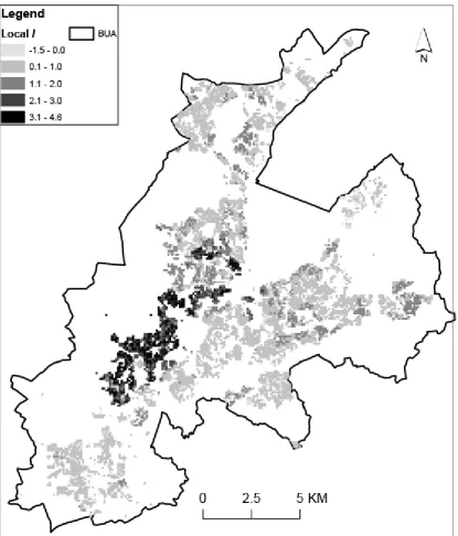
Figure 4 shows local I for a locally-adaptive bandwidth of 20 nearest neighbours (bi-square function). The map suggests that west Belfast has the most obvious clusters – these are locations where there are spatial concentrations of values which depart markedly from the mean. Examination of Figure 1 supports this to some degree, although in some areas, particularly in the mid west and parts of the east, more strongly positive values would be expected to reflect the consistently small percentage of Catholics (and thus consistently large percentages of Protestants) in those areas. In other words, where there are cells with, for example, a large proportion of Protestants surrounded by cells with similar characteristics, the values deviate markedly from the mean and thus large values of local I would be expected.
FIGURE 4 ABOUT HERE
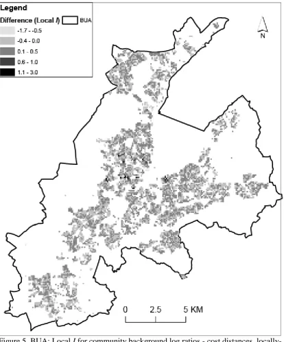
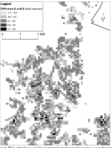
Belfast. Notably, the cost distance derived local I values are markedly larger than those for the conventional kernel in the Protestant-dominated Shankill Road area of west Belfast. The area is apparent in Figure 1 as the band which bisects the two main Catholic-dominated areas of west Belfast. This area is in the southern third of Figure 6 – which shows the same values as in Figure 5, but with greater detail for this particular part of west Belfast. This map indicates that using cost distances (which include information on the peace walls shown in Figure 6), correctly reduces the negative spatial autocorrelation which is evidenced in some of these areas using a conventional kernel. In addition, and as suggested in principle by Figure 3, use of cost surface-derived weights tends to result in more positive values of local I at locations close to the peace walls. Therefore, the cost surface weights appear to more accurately reflect clustering either side of the peace walls than do conventional weights which suggest interactions across the peace walls.
FIGURE 5 ABOUT HERE
FIGURE 6 ABOUT HERE
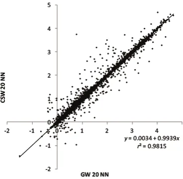
Local I values for community background log ratios with a locally-adaptive bandwidth of 20 nearest neighbours based on Euclidean distances are strongly related to those derived using cost distance weights, as indicated by Figure 7, which plots one set of values against the other. While most values are similar, there are clearly a large number of values of local I for cost surface weights which are larger (more positive) than the equivalent values obtained using the conventional geographical weights and there are large differences for cells close to peace walls. As the number of nearest neighbours increases, there is a greater potential for difference between values of local I derived using conventional weighting schemes or cost distances.
FIGURE 7 ABOUT HERE
Global I is computed using raw percentages and log ratios. Table 2 gives Moran’s I for Catholics by community background (%) and the community background log ratio. The table includes results for I based on (i) Queen contiguity, (ii) Euclidean distances (with weights determined using the Gaussian weighting scheme and the locally-adaptive square function), and (iii) cost distances (using the inverse of the costs, inverse square, bi-square function, and also time bandwidths with the inverse bi-square of the costs within a set travel time of the focal cell). In addition, Table 2 explores the impacts on I of varying the size of the ‘local neighbourhood’ used for each weighting scheme. The larger values of I for percentages than for log ratios is, at least in part, a function of the addition of one to the counts of Catholics and non Catholics (see Section 2) which reduces variation in the data when computing the latter. However, the results obtained using percentages and log ratios are proportionately similar, when comparing between metrics, weighting schemes, and local neighbourhood definitions. Thus, in this case, the choice of raw percentages or transformed values is of relatively little practical importance.
TABLE 2 ABOUT HERE
the bi-square function, defined in Equation 3, is used) than it is for large bandwidths. The smallest values of I are for the fixed bandwidths of 500m and 1000m, as these cover larger areas than the other weighting schemes considered.
Next, we can compare the results obtained with Euclidean and cost distance metrics. The values of I for the cost distance metric with weights determined by the locally adaptive (bi-square) kernel are in line with those obtained using the Euclidean distance metric with the same weighting function. Thus, for global I, the choice of the Euclidean distance metric or a cost distance metric does not have major implications in terms of the results. The values of I for a given number of nearest neighbours are similar regardless of the weighting schemes applied to cost distances (inverse distance with k=1 and k=2, and the bi-square kernel), although the difference between the three sets of values for the 20 nearest neighbours emphasizes the differences in weights assigned to more distant observations by the two weighting schemes (that is, the decay is more ‘rapid’ in one case than the other). The time bandwidths are conceptually useful in that the feasibility of a trip, and thus interactions, are usually judged by travel time and not by distance.
In summary, the results for local I clearly illustrate the potential advantages of using a weighting scheme based on local cost surfaces. For global I, the results are less clear and, while cost distance weights are conceptually superior to weights based on Euclidean distances, the values of global I are close to one another for similar neighbourhood sizes, irrespective of the use of Euclidean or cost distances for weighting – although the differences are likely to increase as the size of the neighbourhood increases.
8. Discussion and conclusions
This paper demonstrates that it is possible to derive a gridded local friction surface that sensibly takes account of vector line features, even allowing for the fact that the conversion of vector features to a grid surface is inevitably approximate. Given gridded friction values, a local cost surface can be computed and used to derive a weighting scheme for the measurement of spatial autocorrelation using gridded data. Such an approach is a conceptual improvement on simple geographical weighting schemes where, in the case of gridded data, interactions between individuals in particular areas are usually considered to be a simple function of Euclidean distance between cells. Cost surfaces and distance decay functions share the same weakness in that there are innumerable possible ways of defining them. But, it seems likely that assumptions of isotropy and spatial homogeneity in simple distance decay functions will hold in very few situations. Functions of Euclidean distance may allow the assessment of the spatial configuration of a population subgroup, but they will rarely provide a meaningful model of interactions, which must be a core consideration if assessment of population clustering (as an example) is the objective. With cost surfaces, weights can vary with direction (e.g., travel along a road) across grid cells, and with location (weights may be different with respect to the neighbourhood of particular cells). In this analysis, alternative approaches to cost surface modelling can be seen as a hierarchy where costs from location i can be computed (i) to all other cells, (ii) within a time bandwidth, or (iii) to a pre-defined number of neighbouring cells. The first approach was not considered because of the high computational cost and because a local approach is sufficient to determine weights, while both the second and third were applied.
least allow a clear demonstration of the benefit of cost surface-based weights which correctly suggest positive autocorrelation by community background on both sides a of peace wall. In addition, the cost distance-based weights result in more strongly positive spatial autocorrelation in some areas where dominantly Catholic neighbourhoods border dominantly Protestant neighbourhoods and where the two are not physically divided by peace walls. There is an implicit assumption behind the approach employed here that all persons have access to transport and that they would take the ‘optimal’ route, in terms of travel time, from one location to another. Although it is obvious that particular groups are likely to have differential access to, in particular, cars (according to, for example, age or socioeconomic profile) it is argued that cost surfaces are more suggestive of potential interactions than are simple functions of Euclidean distance.
The analysis shows that global I is relatively insensitive to the type of decay function and neighbourhood size (at least for the neighbourhood sizes defined here), and that results are similar for weighting schemes based on Euclidean and cost distance metrics. Analyses based on raw percentages and log ratios are, in relative terms, very similar. Despite this, a statistically valid approach based on log ratios is preferred here to direct analysis of percentages. In the case of local I, large differences between results obtained using Euclidean and cost distance metrics were observed at some locations, most notably in close proximity to peace walls. Thus, the use of a cost distance metric is likely to be of value where there are locally important features which either impede or facilitate travel, but more research is required to more fully assess the practical implications of different choices of distance metric for particular applications.
The availability of data sources indicating where individuals are at particular times of day offers the opportunity to more accurately model interactions using cost surfaces, and thus to refine the approach presented here. The Economic and Social Research Council-funded project ‘Population24/7: Space-time specific population surface modelling’ (Cockings et al. 2010) is making use of data from the UK Census of Population and other sources relating to workplaces, educational and leisure establishments and healthcare facilities to generate population surfaces referring to specific times of day. Such data sources could potentially be used to represent directly population interactions or to refine cost surfaces by representing the magnitude of population movements between locations or by the use of particular modes of transport.
In the present study, gridded data population were available. For users who have access only to data for irregular zones there are the options of (i) converting the data to a grid using some form of areal reallocation procedure (for example, using an approach such as that applied by Martin et al. 2011) or (ii) adapting the present approach to work directly with irregular zones. Even 100m cells, as applied here, represent a considerable loss of detail – each cell in a friction surface can only be associated with one mode of transport, and thus one cost. In reality, the transport system and the precise connections between its component parts may be very complex even over an area of 100m by 100m. There is scope to refine the approach given more detailed data, but cost surfaces are, in principle, a logical way of representing interactions and the approach presented here presents, it is argued, an improvement over standard geographical weighting schemes.
to represent travel speeds in different areas. In addition, spatial autocorrelation in other variables could be explored. When measures making use of cost distance-based weights are compared to those using standard geographical weights, the differences will be larger for some variables than for others. For example, religion either side of a peace wall is likely to be more different than for example, unemployment rates. Therefore, in the Northern Ireland case, use of a cost distance-based weighting scheme may make more difference at some locations for religion than for employment.
Cost surface-derived weights are applicable in contexts other than the measurement of spatial autocorrelation and applications in geographically weighted regression (GWR) are currently being explored. Cost distances have been used as covariates in GWR analyses, but their use as weights is likely to prove beneficial where functions of Euclidean distance are not appropriate. In any application making use of gridded data and geographical weighting functions, local cost distances could be used to determine weights. These include interpolation, spatial filtering, and spatial regression (e.g., spatial autoregressive models or GWR). The present study provides a platform on which future analyses of these kinds can be built.
Acknowledgements
The Census Office (part of the Northern Ireland Statistics and Research Agency – NISRA) are thanked for providing the grid square data. Data source: Northern Ireland Statistics and Research Agency Website: www.nisra.gov.uk. Crown copyright material is reproduced with the permission of the Controller of HMSO. The analysis made use of products derived from OSNI (Ordnance Survey Northern Ireland) road network data while the author was employed by Queen’s University Belfast. This material is Crown Copyright and its provision under the Northern Ireland Mapping Agreement is acknowledged. The two anonymous referees are thanked for their very helpful remarks on the paper. In addition, Paul Williamson (associate editor), is sincerely thanked for his detailed comments on the structure and content of the paper – they improved the paper considerably.
References
Aitchison, J. (1986) The Statistical Analysis of Compositional Data. London: Chapman and Hall.
Anselin, L. (1995) Local indicators of spatial association — LISA. Geographical Analysis, 27, 93–115.
Anselin, L., Syabri, I., and Kho, Y. (2006) GeoDa: an introduction to spatial data analysis. Geographical Analysis, 38, 5–22.
Bivand, R., Hauke, J. and Kossowski, T. (2013) Computing the Jacobian in Gaussian spatial autoregressive models: an illustrated comparison of available methods. Geographical Analysis, 45, 150–179.
Brown, L. A. and Chung, S.-Y. (2006) Spatial segregation, segregation indices and the geographical perspective. Population, Space and Place, 12, 125–143.
Chang, K.-T. (2010) Introduction to Geographic Information Systems, 5th edition. New York:
McGraw.
Cliff, A. D. and Ord, J. K. (2009) What were we thinking? Geographical Analysis, 41, 351– 363.
Cockings, S., Martin, D. and Leung, S. (2010) Population 24/7: building space-time specific population surface models. In Proceedings of the GIS Research UK 18th Annual Conference GISRUK 2010 (eds M. Hakley, J. Morley and H. Rahemtulla), pp. 41–48. London: University College London.
Dijkstra, E. W. (1959) A note on two problems in connection with graphs. Numerische Mathematik, 1, 269–271.
Filzmoser, P., Hron, K. and Reimann, C. (2009) Univariate statistical analysis of environmental (compositional) data: problems and possibilities. Science of the Total Environment, 407, 6100–6108.
Fotheringham, A. S., Brunsdon, C. and Charlton, M. (2002) Geographically Weighted Regression: The Analysis of Spatially Varying Relationships. Chichester: John Wiley and Sons.
Gatrell, A. C. (1983) Distance and Space. Oxford: Clarendon Press.
Getis, A. and Aldstadt, J. (2004) Constructing the spatial weights matrix using a local statistic. Geographical Analysis, 36, 90–104.
Gonzalez, J. R., del Barrio, G. and Duguy, B. (2008) Assessing functional landscape connectivity for disturbance propagation on regional scales — A cost-surface model approach applied to surface fire spread. Ecological Modelling, 211, 121–141.
Greenberg, J. A., Rueda, C., Hestir, E. L., Santos, M. J. and Ustin, S. L. (2011) Least cost distance analysis for spatial interpolation. Computers and Geosciences, 37, 272–276.
Howey, M. C. L. (2007) Using multi-criteria cost surface analysis to explore past regional landscapes: a case study of ritual activity and social interaction in Michigan, AD 1200– 1600. Journal of Archaeological Science, 34, 1830–1846.
Laxman, K. K; Rastogi, R. and Chandra, S. (2010) Pedestrian flow characteristics in mixed traffic conditions. Journal of Urban Planning and Development, March 2010, 23–33.
LeSage, J. P. (2008) An introduction to spatial econometrics. Revue d'Économie Industrielle, 123, 19–44.
LeSage, J. and Pace, R. K. (2009) Introduction to Spatial Econometrics. Boca Raton: Chapman & hall/CRC.
Lloyd, C. D. (2010a) Exploring population spatial concentrations in Northern Ireland by community background and other characteristics: an application of geographically weighted spatial statistics. International Journal of Geographical Information Science, 24, 1193– 1221.
Lloyd, C. D. (2011) Local Models for Spatial Analysis, 2nd edition. Boca Raton: CRC Press.
Lloyd, C. D. (2012) Analysing the spatial scale of population concentrations in Northern Ireland using global and local variograms. International Journal of Geographical Information Science, 26, 57–73.
Lloyd, C. D., Pawlowsky-Glahn, V. and Egozcue, J. J. (2012) Compositional data analysis for population studies. Annals of the Association of American Geographers, 102, 1251–1266.
Lowe, J. C. and Moryadas, S. (1975) The Geography of Movement. Boston: Houghton Mifflin Company.
Martin, D. J., Lloyd, C. D. and Shuttleworth, I. G. (2011) Evaluation of gridded population models using 2001 Northern Ireland Census data. Environment and Planning A, 43, 1965– 1980.
Massey, D. S. and Denton, N. A. (1988) The dimensions of residential segregation. Social Forces, 67, 281–315.
Moran, P. A. P. (1950) Notes on continuous stochastic phenomena. Biometrika, 37, 17–23.
Noonan, D. S. (2005) Neighbours, barriers and urban environments: are things ‘different on the other side of the tracks’? Urban Studies, 42, 1817–1835.
Patuelli, R., Griffith, D. A., Tiefelsdorf, M. and Nijkamp, P. (2012) Spatial filtering methods for tracing space-time developments in an open regional system: experiments with German unemployment data. In Societies in Motion: Innovation, Migration and Regional Transformation (eds A. Frenkel, P. Nijkamp and P. McCann), pp. 247–268. Cheltenham: Edward Elgar, Northampton.
Poole, M. A. and Doherty, P. (1996) Ethnic Residential Segregation in Northern Ireland. Coleraine: University of Ulster.
Poulsen, M., Johnston, R. and Forrest, J. (2010) The intensity of ethnic residential clustering: exploring scale effects using local indicators of spatial association. Environment and Planning A, 42, 874–894.
Ravenstein, E. G. (1885) The laws of migration. Journal of the Royal Statistical Society, 48, 167– 235.
Ravenstein, E. G. (1889) The laws of migration. Journal of the Royal Statistical Society, 52, 241– 305.
Shuttleworth, I. G. and Lloyd, C. D. (2009) Are Northern Ireland’s communities dividing? Evidence from geographically consistent Census of Population data, 1971–2001. Environment and Planning A, 41, 213–229.
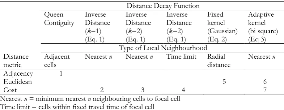
Distance Decay Function Queen
Contiguity Inverse Distance (k=1) (Eq. 1) Inverse Distance (k=2) (Eq. 1) Inverse Distance (k=2) (Eq. 1) Fixed kernel (Gaussian) (Eq. 2) Adaptive kernel (bi square) (Eq 3) Type of Local Neighbourhood
Distance
metric Adjacent cells Nearest n Nearest n Time limit Radial distance Nearest n
Adjacency 1
Euclidean 5 6
Cost 2 3 4 7
Nearest n = minimum nearest n neighbouring cells to focal cell Time limit = cells within fixed travel time of focal cell
[image:20.595.108.568.70.249.2]Radial distance = cells within fixed distance of focal cell
Table 1. Distance metrics and corresponding weighting schemes.
Weighting scheme Neighbourhood Catholics
(distance metric + distance
decay function) Type Size % Log ratio
(1) Queen contiguity Adjacent cells 0.911 0.875
(5) Euclidean distance, Fixed
kernel bandwidth (Gaussian) Radial distance 100m 500m 0.904 0.677 0.867 0.646
1000m 0.515 0.486
(6) Euclidean distance, Adaptive kernel bandwidth (bi-square)
Nearest n 6 0.922 0.886
10 0.914 0.878
20 0.893 0.858
(2) Cost distance, Inverse
distance, k=1 Nearest n 10 6 0.916 0.906 0.880 0.871
20 0.886 0.852
(3) Cost distance, Inverse
distance, k=2 Nearest n 10 6 0.919 0.912 0.882 0.876
20 0.899 0.864
(7) Cost distance, Adaptive
kernel bandwidth (bi-square) Nearest n 10 6 0.923 0.913 0.886 0.877
20 0.890 0.856
(4) Cost distance, Inverse distance, k=2 (time bandwidth)
Time limit 1 minute 0.904 0.867
5 minutes 0.838 0.808
10 minutes 0.819 0.789
[image:20.595.92.553.334.638.2]