Direct Predictive Current-error Vector Control for a
direct Matrix Converter
Manjusha Vijayagopal
1, Cesar Silva
2, Lee Empringham
1, Liliana de Lillo
1 1. The University of Nottingham, UK, NG7 2RA2. Federico Santa María Technical University, Valparaiso, Chile
Abstract—This paper proposes a novel control strategy for matrix converters which is coined “Direct Predictive Current-error Vector Control”. The proposed control method retains the advantageous features of both a modulation scheme and of a predictive based controller. The result is a controller that is capable of good dynamic performance and steady state response with fixed switching frequency operation. Control of load and input currents of a direct matrix converter using the proposed method is demonstrated in this paper by simulation and experimental results.
Keywords—direct matrix converter, matrix converter, current control, modulation
I. INTRODUCTION
Matrix converters have been a topic of growing interest for the decades since the development of a control and modulation algorithm for the same by Alesina and Venturini in 1989 [1]. The mathematical approach to solving the modulation problem developed by Alesina and Venturini was later augmented by the Space Vector Modulation (SVM) strategy introduced by Huber and Borojevic in 1995 [2]. In this method, the available voltages for each switching state of the converter is represented in terms of space phasors and a combination of these vectors with specific duty cycles are applied to obtain the desired output voltage. SVM together with conventional proportional-integral (PI) controllers were used to control matrix converters for a variety of applications such as drives [3, 4] and power supplies [5]. Other control methods such as Model Predictive Control (MPC) are being widely researched to control power converters and has also been used to control matrix converters [6, 7]. The compact design of the converter due to the absence of a DC link capacitor is seen as a major advantage for these converters and exploiting this feature to design compact drives is becoming popular [8].
MPC is a predictive control based algorithm where the model of the system together with system variables such as input and output voltages and currents are used to predict its behavior at future instants [9]. For power converters, the problem at hand is the selection of switching states according to the current control demand, resulting in an optimization with respect to a finite set of possible actuations (FS-MPC). Since FS-MPC is based on the predictions of each possible switching state, it lacks a modulation method that generates duty cycles for the voltage vectors. MPC chooses the switching state that results in minimum error between the desired output and the predicted output in the next sampling instant. The predictions of the control variable for all the available switching states for a power converter are calculated prior to the optimization algorithm. MPC involves minimizing a pre-defined cost function and selecting the switching state that results in the least error. A cost function is typically the quadratic error between the reference variable and the control variable at the future instant [10]. It can be expressed in general terms as shown in (1).
𝐺 = (𝑥𝑟𝑒𝑓(𝑘 + 1) − 𝑥(𝑘 + 1))2 (1)
Since there is no modulation involved, only one vector is applied throughout the entire sampling interval. It is therefore highly likely that one switching state may result in generating the minimum error for more than one sampling interval. This leads to a variable switching frequency operation. A typical frequency spectrum of a waveform generated by MPC will contain low frequency harmonics with the switching harmonics spread over a wide band, without the typical concentrated spectral lines near a carrier frequency and its multiples as seen with PWM. Even though MPC provides fast transient response, the quality of the controlled waveforms in steady state are poor compared to the case where a modulation technique together with a suitable PI controller are involved. The quality also diminishes drastically with an increase in length of the sampling interval. The difficulty in creating a design of input filter for a matrix converter will be greatly increased by the absence of a fixed frequency switching harmonics as the filter cut off frequency and response to filter resonance cannot be calculated accurately. On the other hand, conventional controllers such as the PI controllers together with space vector modulation (SVM) can result in high quality input and output waveforms. However, one of the disadvantages of this type of control scheme is the inability to provide transient response within a few sampling intervals as is the case with MPC.
discussed in detail in [19] with M2PC clearly showing superior performance compared to MPC. While [14, 15, 19] discuss load current control by a modulated predictive control for a direct matrix converter, they do not include control of supply currents, which is an important control objective for a matrix converter.
(a)
(b)
Fig 1. (a) Direct matrix converter system, (b) Input current and output voltage vectors of a MC
An attempt to control the supply side by input reactive power minimization simultaneously with the load current control for a direct matrix converter drive is discussed in [18] using modulation of the best switching states based on the absolute, i.e. scalar current error, M2PC [13]. The method shown in [18] relies on an additive term of the cost function and produces significant improvements with respect to FS-MPC, but the input current still presents significant ripple with respect to that obtained with SVM.The main difference between M2PC and the proposed control method is in the determination of the duty cycles of the voltage vectors. In M2PC the main objective was to achieve a response with fixed switching frequency by modulating between the vectors that results in minimum magnitude of current error. In [19], voltage vectors corresponding to each sector are selected from a look up table based on the vector sequence employed in a Space Vector Modulation (SVM) technique for direct matrix converters. This consists of a sequence of four vectors for each output voltage sector. The M2PC algorithm chooses the set which results in the minimum magnitudes of load current error and modulate between them heuristically which has been found to be a suboptimal solution. This method does not consider the direction of the error vectors and hence the calculated duty cycles are inaccurate in the sense that no effort is made to use vectors whose errors counteract each other. On the other hand, the M2PC method does achieve constant switching frequency and small total errors that at the time were an improvement with respect to the state of the art.
Further research has led to the current modulated predicted method ((DPCVC) that considers the complex nature of the predicted current errors, choosing four active voltage vectors corresponding to a particular sector of the well-known voltage hexagon. These vectors produce current errors that, when properly modulated, achieve zero total current error, i.e. optimum current error. T his effectively leads to the same vector sequence employed in a Space Vector Modulation (SVM) technique for direct matrix converters,
1 2
3
4
5
6 V1 V2 V3
V4
V5 V6
± 1, ±2, ±3
± 7, ±8, ±9 ± 4, ±5, ±6
1 2 3
4
5 6
I1 I2
I3
I4
I5
I6
± 1, ±4, ±7 ± 3, ±6, ±9
± 2, ±5, ±8
but achieves optimum response in the sense that the current error reaches zero for the input and output current in one modulation period, provided that the converter has sufficient actuation capability. For the direct matrix converter to achieve zero current error in the input and output, the initial current error should be sufficiently small, resulting in a linear modulation. When the initial current error is not small enough, the method chooses less number of active vectors, effectively saturating the modulator, leading to the smallest possible (optimum) current error at the end of the modulation period. In [20] it has been shown that, for the case of voltage source inverters, to reach the zero output current error, which is the optimum in linear modulation mode, the vector nature of the error must be considered in the calculation of the duty cycles. In this work, this principle is extended to a direct matrix converter to develop a predictive control strategy that is capable of input and output current control of a direct matrix converter together with a fixed switching frequency operation using a vector modulation of the predicted input and output current errors.
II. DIRECT MATRIX CONVERTER
A direct matrix converter (MC) shown in Fig.1 (a) is an AC-AC converter that is capable of generating variable voltage and frequency output from a variable voltage and frequency input. A MC consists of nine bidirectional switches connected in the form of a matrix, enabling bidirectional power flow in the converter [21]. An interesting feature of this converter is the direct power conversion in the absence of an intermediate DC-link for energy storage. The only passive component that is part of the converter is a small input LC filter that is only required to filter out the switching frequency harmonics on the supply side currents. The output of the converter is normally connected to an inductive load such as an induction machine.
A. Modulation of Matrix Converter
Modulation of MC has been a topic of interest in academia for a number of years and various methods have been proposed to achieve this aim. A commonly used modulation method is SVM and is capable of generating sinusoidal output voltages and input currents with the possibility for input power factor control. For a MC, nine switches can be turned on and off in 27 different combinations resulting in 27 switching states or voltage vectors. Out of the 27 states, 6 of them results in rotating vectors and hence are not used for modulation. The 21 input current and output voltage vectors for a MC are shown in Fig. 1(b). Due to the triple redundancy of the zero vectors, the 21 switching states can be reduced to 19 output voltage and input current vectors. The output voltage sectors, Kv and input current sectors, Ki ranging from 1 to 6 are also shown in Fig. 1(b). The main output voltages of the MC can be derived directly from Fig. 1(a) and expressed in terms of the supply voltages as shown in (2).
[ Va(𝑡)
Vb(𝑡)
Vc(𝑡)
]=[
SAa SBa SCa
SAb SBb SCb
SAc SBc SCc
] [ VA(𝑡)
VB(𝑡)
VC(𝑡)
] (2)
The input currents of the converter can be expressed in terms of the load currents as shown in (3).
[
Iia(𝑡)
Iib(𝑡)
Iic(𝑡)
]=[
SAa SBa SCa
SAb SBb SCb
SAc SBc SCc
] 𝑇
[
Ia(𝑡)
Ib(𝑡)
Ic(𝑡)
] (3)
where Sij is the switching function with i=A,B,C and j= a,b,c.
This mathematical model of the converter is utilized to determine the instantaneous output voltage and input current vectors that are used in the modulation of the converter. In SVM, four active vectors and three zero vectors are used to obtain the reference output voltage while controlling the input current angle [22].The duty cycles for the application of these vectors are calculated using equations (14) to (17) in [22].
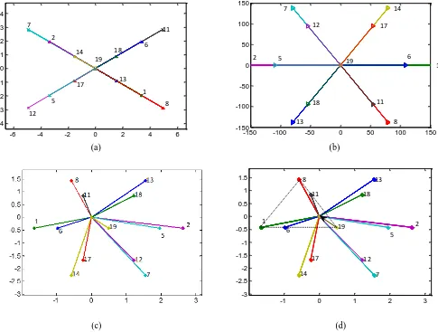
(a) (b)
(c) (d)
Fig 2.(a) Output voltage vectors (b) Input current vectors (c) Output current error vectors of a MC for Ki=1 and (d) Arrangement of 12 arbitrary load current error
vectors in 𝛼𝛽plane
controller gains can be tuned based on the system requirements. However, the transient response of PI controllers is relatively slow when compared to predictive based controllers which minimizes the response time. Controllers such as finite control set MPC on the other hand can deliver fast transients while the steady state response is compromised [24]. Also, as previously discussed, FS-MPC results in variable switching frequency operation which makes it difficult to design an input filter accurately in the case of a matrix converter[15].
III. PROPOSED CONTROL METHOD
Direct Predictive Current-error Vector Control (DPCVC) is based on predictive control and includes a modulation scheme. It is developed to overcome the drawbacks of FS-MPC while maintaining its advantageous features such as fast dynamic response. The proposed method is based on the principle proposed in [21] for a three phase 2-level inverter. The fundamental idea is to consider the current error in its vector form in αβ plane as cost function in order to calculate the duty cycles or application times for the converter switching states. This method does not rely on a pre-defined look-up table to obtain the voltage vector sequence as opposed to M2PC. It considers the load current error vector and selects the four voltage vectors which will result in minimum error using the predictive control algorithm. With this exercise, the algorithm chooses four vectors that satisfy the load and supply current sector requirements. The duty cycles for these vectors are calculated using the constraint equations for both load current and supply current control.
The basic principle of DPCVC is based on the current error vectors formed by each switching state of the converter. For example, for current control, the load current-error vectors when plotted in αβ plane results in a hexagon similar to that of the voltage vectors for each switching state; with error produced by the zero vector as the center. For a matrix converter, to attain control of both load currents and input current, four active vectors and three zero vectors will be used for modulation. The output voltage vectors for a direct matrix converter for each switching state are shown in Fig.1(c). In order to simplify the problem at hand and reduce the computation requirement, a pre-selection of certain vectors is made out of the 21 available voltage vectors, using the knowledge of
-1 0 1 2 3
-3 -2.5 -2 -1.5 -1 -0.5 0 0.5 1 1.5 13 1 8 7 2 14 11 6 18 17 5 12 19
-150 -100 -50 0 50 100 150
-150 -100 -50 0 50 100 150 13 1 8 7 2 14 11 6 18 17 5 12 19
-6 -4 -2 0 2 4 6
-4 -3 -2 -1 0 1 2 3 4 13 1 8 7 2 14 11 6 18 17 5 12 19
-1 0 1 2 3
-3 -2.5 -2 -1.5 -1 -0.5 0 0.5 1 1.5 13 1 8 7 2 14 11 6 18 17 5 12 19
-150 -100 -50 0 50 100 150
-150 -100 -50 0 50 100 150 13 1 8 7 2 14 11 6 18 17 5 12 19
-6 -4 -2 0 2 4 6
-4 -3 -2 -1 0 1 2 3 4 13 1 8 7 2 14 11 6 18 17 5 12 19
-1 0 1 2 3
-3 -2.5 -2 -1.5 -1 -0.5 0 0.5 1 1.5 13 1 8 7 2 14 11 6 18 17 5 12 19
-150 -100 -50 0 50 100 150
-150 -100 -50 0 50 100 150 13 1 8 7 2 14 11 6 18 17 5 12 19
-6 -4 -2 0 2 4 6
[image:4.595.61.546.60.427.2]the voltage vectors involved in SVPWM of a matrix converter [22]. This is achieved by determining the desired input current sector based on the information about the supply voltages (and the desired input displacement factor). As this calculation is performed in real time, any unbalance in the supply voltage will be taken into account in the determination of the input current sector and prediction of the output currents. Once the desired input current sector is determined from the supply voltages, the number of available active voltage vectors/switching states for modulation can be narrowed down to 12. For example, in Fig. 1(b), if the desired input current sector is 1 (Ki=1 and unity displacement factor), then the voltage vectors that can produce an input current in that sector are ±3, ±6, ±9, ±1, ±4, ±7. For simplicity, the switching states represented as ±1, ±2, ……., ±9, 0 will be addressed as 1, 2, 3, 4…….18, 19 asshown in Fig. 2(a-d). Thus, the input current vectors and the output voltage vectors for Ki=1 are shown in Fig. 2(a) and Fig. 2(b) respectively. The predicted error of the load currents for the 12 selected vectors can be calculated from the predictive load model. Equations (4) and (5) illustrate this operating principle for a simple RL load.
𝐼𝑗𝑜(𝑘 + 1) = (1 − 𝑅𝑇𝑠
𝐿 ) 𝐼𝑜(𝑘) + 𝑇𝑠
𝐿 𝑉 𝑗
𝑜(𝑘) (4)
𝑒𝑗= 𝐼𝑗𝑜(𝑘 + 1) − 𝐼𝑜(𝑘) (5)
where 𝐼𝑜(𝑘 + 1) and 𝐼𝑜(𝑘) are the load currents at (k+1) and k instants respectively for j={0,1, 2,…….12}.
The error vectors for the 12 selected active switching states are shown in Fig. 2(c). The error vectors form a hexagon (with 19 as the center), similar to the output voltage vectors, but transformed by the load model, which is in general an affine transformation that preserves shape, i.e. composed by a linear function and a translation. In the case of the example, the transformation is given by (4) and (5). From the Fig. 2(c), it is noted that the magnitudes of the error vectors are also varying; as are the voltage vectors used to calculate the predicted load currents.
Based on predictive control algorithm, the objective is to minimize the load current error, making it equal to zero if possible. Therefore the target point to achieve when the load current errors are plotted is the origin of the plane. The control problem is then to find the linear combination of five vectors (active and zero) which will result in zero load current error, as illustrated by Fig. 2 (d), together with a controlled input current angle
[image:5.595.191.405.371.564.2]
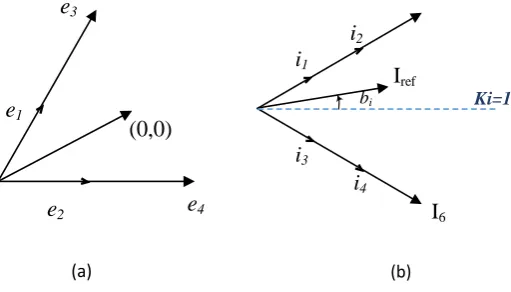
Fig 3. Load current error vectors of a MC
To explain the control procedure, a general case is considered where there are 12 arbitrary error vectors named e1, e2 ….e12 and the error vector obtained with the zero voltage vector, e0. The arrangement of these vectors in the 𝛼𝛽 co-ordinate plane can be shown as in Fig. 3. The origin of the plane, (0,0) is the target point which will correspond to load current reference tracking. The control problem is then to find a set of vectors that are capable of producing zero load current error when applied with their respective duty cycles. The procedure to achieve this can be explained based on Fig. 3 where the target point can be achieved by the linear combination of error vectors 𝑒2,𝑒3, 𝑒8, 𝑒9 (shown in red) and 𝑒0 in a certain proportion. A solution exists only if the target (origin) lies within the triangle formed by any five vectors. If the target lies outside the triangle defined by two larger vectors and the zero vector, it is considered that the over modulation condition has been reached and different measures need to be taken to address it.
e
1e
2e
3e
4e
5e
6α
β
e
0e
9e
8 (0,0)e
7e
12e
11The relevant triangle or consecutive set of vectors can be obtained from the conditions mentioned in [20] for each consecutive set of vectors. For example, if the vectors that form the vertices of the hexagon are considered, for every pair of consecutive vectors like (1,2), (2,3), (3,4), (4,5), (5,6), (6,1) a linear combination of 𝑒𝑥, 𝑒𝑦 and 𝑒0 exists if the following conditions are met.
(𝑒𝑥− 𝑒0) × (−𝑒0) · (𝑒𝑦− 𝑒0) × (−𝑒0) ≤ 0 (6)
(𝑒𝑥− 𝑒0) · (−𝑒0) > 0 (7)
(𝑒𝑦− 𝑒0) · (−𝑒0) > 0 (8)
where <·> is the dot product operator and < X> is the cross product operator.
The set of vectors that satisfy the conditions in (6-8) is selected for modulation. In the case of Fig. 3, this will result in vectors 𝑒2,𝑒3, 𝑒8, 𝑒9and e0. . Once the consecutive vectors in the vertices of the hexagon are determined, the inner vectors with the same phase angle are selected resulting in four active vectors to modulate. In general terms, the five error vectors will be renumbered and referred to as 𝑒1, 𝑒2, 𝑒3, 𝑒4and e0 with suffix ‘1,2,3 and 4’ representing the active vectors and suffix ‘0’ to the zero vector. This set of vectors is combined to achieve zero current error as shown in Fig. 4 (a). To control the input current angle, it is assumed that the desired input current is in phase with the supply voltage. The procedure then is to force the angle of the input current to be identical to that of the supply voltage. This is possible by considering two additional constraint equations which translates the desired behavior of the input current. The selected four active vectors result in input currents𝑖⃗⃗⃗⃗ , 𝑖1 ⃗⃗⃗⃗ , 𝑖2 ⃗⃗⃗⃗ 3 and 𝑖⃗⃗⃗⃗ 4 as shown in Fig. 4(b) that need to be combined appropriately.
Fig 4. (a) Load current error and (b) Input current vectors for Ki=1
The target vector in the case of load current error vectors is the origin as shown in Fig. 4 (a) whereas the target vector for the input current is represented by the angle of Iref. The reference input current vector angle, bi is obtained from the supply voltage and the magnitude of this vector is unknown. From Fig. 4(b) it is evident that the reference current vector, Iref can be obtained by the combination of 𝑖⃗⃗⃗⃗ 1 and 𝑖⃗⃗⃗⃗ 3 or 𝑖⃗⃗⃗⃗ 2 and𝑖⃗⃗⃗⃗ 4. This will constitute the constraint equations for input current angle control. For load current control, the origin of the plane needs to be obtained by a combination of 𝑒⃗⃗⃗⃗ , 𝑒1 ⃗⃗⃗ , 𝑒2 ⃗⃗⃗⃗ 3 and𝑒⃗⃗⃗⃗ 4. This can be represented in vector form as shown in equation (9)
𝑑1 𝑒⃗⃗⃗⃗ + 𝑑1 2 𝑒⃗⃗⃗ + 𝑑2 3 𝑒⃗⃗⃗⃗ + 𝑑3 4 𝑒⃗⃗⃗⃗ + 𝑑4 0 𝑒⃗⃗⃗⃗ = 0 (9)0
The input current vectors can be combined to obtain a current vector with the reference angle by considering the dot product between the averaged short and long input current vectors and a perpendicular vector to the reference as shown in equation (10-11). This allows to arbitrarily force a phase angle bi to the input current vector, allowing to control the input reactive power.
(𝑑1 𝑖⃗⃗⃗⃗ + 𝑑1 3 𝑖⃗⃗⃗⃗ ) ∙ 𝑗𝑒3 𝑗𝑏𝑖= 0 (10)
(𝑑2 𝑖⃗⃗⃗⃗ + 𝑑2 4 𝑖⃗⃗⃗⃗ ) ∙ 𝑗𝑒4 𝑗𝑏𝑖 = 0 (11)
Equation (9) can be divided into 𝛼𝛽 components as shown in (12) and (13) and the relation for input current angle control can be expanded to obtain (14) and (15). The duty cycles for the selected vectors needed to achieve the target for load current error and
Ki=1
I
refI
6 bii
1i
2i
3i
4(0,0)
e
1e
3e
2e
4(a) (b)
Ki=1
I
refI
6 bii
1i
2i
3i
4(0,0)
e
1e
3e
2e
4 [image:6.595.169.425.316.462.2]input current simultaneously. Finally, the duty cycles for the selected vectors including the zero vector sum to 1 as shown in equation (16). Hence the five duty cycles can be obtained by solving the set of linear equations (12-16).
(𝑒1∝− 𝑒0∝). 𝑑1+ (𝑒2∝− 𝑒0∝). 𝑑2+(𝑒3∝− 𝑒0∝). 𝑑3+ (𝑒4∝− 𝑒0∝). 𝑑4= −𝑒0∝ (12)
(𝑒1𝛽− 𝑒0𝛽). 𝑑1+ (𝑒2𝛽− 𝑒0𝛽). 𝑑2+(𝑒3𝛽− 𝑒0𝛽). 𝑑3+ (𝑒4𝛽− 𝑒0𝛽). 𝑑4= −𝑒0𝛽 (13)
(−𝑖1∝𝑠𝑖𝑛(𝑏𝑖) + 𝑖1𝛽𝑐𝑜𝑠(𝑏𝑖)). 𝑑1+ (−𝑖3∝𝑠𝑖𝑛(𝑏𝑖) + 𝑖3𝛽𝑐𝑜𝑠(𝑏𝑖)). 𝑑3= 0 (14)
(−𝑖2∝𝑠𝑖𝑛(𝑏𝑖) + 𝑖2𝛽𝑐𝑜𝑠(𝑏𝑖)). 𝑑2+ (−𝑖4∝𝑠𝑖𝑛(𝑏𝑖) + 𝑖4𝛽𝑐𝑜𝑠(𝑏𝑖)). 𝑑4= 0 (15)
𝑑1+ 𝑑2+ 𝑑3+ 𝑑4+ 𝑑0= 1 (16)
where 𝑒1
, 𝑒
2, 𝑒
3and 𝑒
4 are the four output current error predictions , i1, i2, i3 and i4 are the predicted input current vectors obtained by the selected four switching states and 𝑑1, 𝑑2, 𝑑3, 𝑑4 and 𝑑0are the duty cycles for each vector. If 𝑑1+ 𝑑2 + 𝑑3+ 𝑑4> 1, it means the zero error target point is outside the hexagon formed by the predicted errorsas in the case of over modulation. In this case, the best actuation to drive the output current to the target point is given by the modulation of the two larger active vectors only. This can be achieved by readjusting the duty cycles for the larger vectors using equations (17-18) and the duty cycles for all other vectors are fixed to zero. This affectively saturates the voltage actuation of the matrix converter to its maximum physical value that minimizes the output current error. 𝑑′1 = 𝑑1 𝑑1+ 𝑑2 (17)𝑑′2= 𝑑2 𝑑1+ 𝑑2 (18)
The resulting voltage vector, assuming the sum of duty cycles < 1, will be a combination of the four active vectors applied for their respective duty cycles and can be expressed as in (19). 𝑣0= 𝑑1 𝑣1+ 𝑑2 𝑣2 +𝑑3 𝑣3+ 𝑑4 𝑣4 (19)
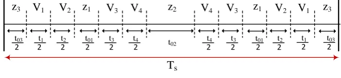
The resulting voltage vectors and duty cycles are applied to the MC in a pre-defined pattern as in the case of SVM [22]. The double-sided switching pattern for MC in this case is shown in
[image:7.595.121.472.477.558.2]Fig. 5.
Fig 5. Double sided switching pattern for MC
If supply current control is not required, this control method can be simplified to control the load. The initial procedure is similar to the previous case where the input current sector is determined and 12 active voltage vectors are selected. In that case, for load current control, the problem becomes very similar to that of a 2-level inverter with five switching states (two active and three zero vectors) to modulate with, if we only consider the vectors in the outer hexagon as shown in Fig. 6.
T
sV
1z
3z
1z
2z
1z
32 t01
2 t2
2 t1
2 t3
t4
2 t02
t4
2 t3
2 t01
2 t2
2 t1
2 t03
2
t03
2
V
3V
3V
4Fig 6. Output voltage vectors of matrix converter
Out of the 12 voltage vectors, only the six active voltage vectors with higher magnitude forming the outer hexagon (shown in red) are considered for modulation. In order to select the two active vectors to modulate, the output current error vectors for each switching state are plotted as shown in Fig. 7.
Fig 7. Output current error in 𝛼𝛽 plane
Based on the predictive control algorithm, the objective is to minimize or obtain zero load current error. Therefore the target is the origin of the plane. The control problem is then to find the linear combination of three vectors which will result in zero load current error. In Fig. 7, this is obtained by the linear combination of predictions 𝑒2, 𝑒3 and 𝑒0 in a certain proportion. A solution exists only if the target (origin) lies within the triangle formed by the two consecutive vectors. If the target lies outside the triangle, it is considered to be in the over modulation condition and the same technique summarized by (17-18 ) can be applied to address it. The relevant triangle or consecutive set of vectors can be obtained from conditions mentioned in equations (6-8) for each pair of consecutive vectors.For every pair of consecutive vectors like (1,2), (2,3), (3,4), (4,5), (5,6), (6,1) a linear combination of 𝑒𝑥, 𝑒𝑦 and 𝑒0exists if equations (6-8) are satisfied. Then,
𝑑1 𝑒⃗⃗⃗⃗⃗ + 𝑑𝑥 2 𝑒⃗⃗⃗⃗ + 𝑑𝑦 0 𝑒⃗⃗⃗⃗ = 0 (20)0
𝑑1+ 𝑑2+ 𝑑0= 1 (21)
where 𝑒𝑥 , 𝑒𝑦 𝑎𝑛𝑑 𝑒0are the output current error predictions for the active and zero vectors. The duty cycle for these vectors can be determined by solving (21), (22) and (23).
(𝑒𝑥∝− 𝑒0∝). 𝑑1+ (𝑒𝑦∝− 𝑒0∝). 𝑑2= −𝑒0∝ (22)
(𝑒𝑥𝛽− 𝑒0𝛽). 𝑑1+ (𝑒𝑦𝛽− 𝑒0𝛽). 𝑑2= −𝑒0𝛽 (23)
This strategy generates accurate duty cycles depending on the instantaneous error predictions and results in fixed switching frequency operation. The control of load currents can be achieved without compromising the input current quality if required. Due
e
1e
2e
3e
4e
5e
6α β
e
0e
xe
y [image:8.595.218.410.266.439.2]to the predictive control based algorithm, this modulation strategy has very fast transients without compromising the switching characteristics of SVM.
IV. SIMULATION RESULTS
[image:9.595.133.465.179.317.2]To validate the theory explained in the previous section, the control of the load currents using DPCVC in a direct matrix converter feeding an RL load has been simulated. The simulations are carried out using the Matlab Simulink environment to implement the control and Plecs Blockset within Matlab to implement the switching and electrical model of the converter. A control block diagram of the proposed method showing all of the functional blocks involved is given in Fig. 8. The input filter consists of a LC filter with a damping resistor parallel to the inductor. The input filter is required to attenuate the switching frequency harmonics.
Fig 8. Control block diagram of the proposed method
A reference current of 8A at 30Hz is demanded from the system. The parameters of the system considered in this simulation test are shown in Table. I.
TABLE I. SYSTEM PARAMETERS
Parameter Value Unit
Filter inducance 0.7 mH
Filter capacitance (delta) 8.3 µF
Damping resistor 15 Ω
Load inductance 3.75 mH
Load resistance 10 Ω
Switching frequency 12.5 kHz
Supply Voltage(rms) 90 V
[image:9.595.196.403.389.534.2]Fig 9. Simulation results: Three phase load current, MC output line voltage and three phase supply currents
From Fig. 9 it is evident that the load currents attains the steady state reference value without any error and the supply currents are sinusoidal. In order to determine the harmonic content of the controlled supply and load currents, Fast Fourier Transform (FFT) of Phase A of the load current and supply current are shown in Fig. 10.
Fig 10. Simulation results: FFT of Phase A load current (top) and supply current of MC (bottom)
The harmonic spectrum of supply and load currents shows the presence of frequencies in the range of 12.5 kHz which is the switching frequency and of its multiples. This proves the fixed switching frequency operation. It can be noted that the steady state waveform quality of this method is comparable to a modulation based approach such as PI control with SVM. The Total Harmonic Distortion (THD) of the supply current and load current waveforms controlled using DPCVC is approximately 3.9% and 1.6% respectively. To demonstrate the fast dynamic response of the DPCVC method, a step in the current demand from 2A to 4A is applied to the converter and the response of the DPCVC is shown in Fig. 11.
0.02 0.04 0.06 0.08 0.1
-10 0 10 L oa d c ur re nt s (A )
0.02 0.04 0.06 0.08 0.1
-200 0 200 M C out put l ine vol ta ge ( V )
0.02 0.04 0.06 0.08 0.1
-5 0 5 Time (s) S uppl y c ur re nt s (A ) Phase A Phase B Phase C Phase A Phase B Phase C
0 0.5 1 1.5 2 2.5 3
x 104 0 0.05 0.1 0.15 0.2 L oa d c ur re nt M a gni tude ( A )
0 0.5 1 1.5 2 2.5 3
Fig 11. Simulation results: Three phase load currents when a step change in the amplitude of the reference is applied at t=0.1s
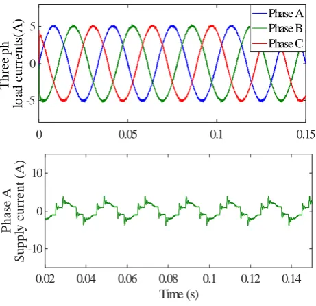
[image:11.595.183.414.262.485.2]A simulation test for load current control without including the supply current control is also performed which uses the outer two active vectors and the zero vectors. The resulting supply current shown in Fig. 12 clearly deteriorates but the output current maintains its sinusoidal waveform, even improving in its ripple content. This condition is similar to the current control mentioned in [19] to obtain controlled load currents for a direct matrix converter.
Fig 12. Simulation results: Three phase load currents and Phase A supply current when supply current control is not included.
The simulation results prove the proposed control theory and that it yields good quality results. The next section explains the application and implementation of the proposed control method on a laboratory prototype of a direct matrix converter.
V. EXPERIMENTAL RESULTS
The proposed control method has been tested for load current control of a direct matrix converter feeding an RL load. A photograph of the experimental setup with the supply, converter and load is shown in Fig. 13. The parameters of the system are the same as shown in Table.1.
0 0.05 0.1 0.15 0.2
Time (s) -5
0 5
3
p
h
L
o
ad
c
u
rr
en
ts
(
A
) Phase APhase B
Phase C
0 0.05 0.1 0.15
Time (s) -5
0 5
T
h
re
e
p
h
lo
ad
c
u
rr
en
ts
(A
) Phase A
Phase B Phase C
0.02 0.04 0.06 0.08 0.1 0.12 0.14
Time (s)
-10 0 10
P
h
a
se
A
S
u
p
p
ly
c
u
rr
e
n
t
(A
Fig 13. Laboratory prototype of a direct matrix converter with RL load
A load current of 5A at 30Hz was demanded from the system with a supply frequency of 50 Hz and the resulting waveforms of three phase load currents, MC output line voltage and the harmonic spectrum of Phase A load current are shown in Fig. 14. The THD of the controlled load current waveform is about 3.97%. As in the case of simulation results, the harmonic spectrum consists of frequencies in the range of switching frequency, 12.5 kHz and its multiples which indicates a fixed switching frequency operation. The controlled supply current waveforms are shown in Fig. 15. It can be noted that the supply currents when included as an objective on the optimization of the cost function are sinusoidal, although some low frequency distortion is observed. This distortion corresponds to the expected excitation of the resonance frequency of 1 kHz and is more noticeable in this experimental result than in the previous simulation result of Fig. 9 due to the low amount of fundamental current being drawn from the supply. The effect of the excitation of the filter resonance frequency can be better appreciated in the simulation result, Fig. 9 and in its spectrum analysis shown in Fig. 10. Despite this distortion, the results seen are more promising than the reactive power and load current control of matrix converter by M2PC discussed in [18].
Fig 14. Experimental results: Three phase load current, MC output line voltage and harmonic spectrum of load currents
0 0.02 0.04 0.06 0.08
-5 0 5
T
h
re
e
p
h
as
e
lo
ad
c
u
rr
en
ts
(A
)
Phase A Phase B Phase C
0 0.02 0.04 0.06 0.08
Time (s)
-100 0 100
M
C
O
u
tp
u
t
l
in
e
v
o
lt
ag
e
(V
)
0 0.5 1 1.5 2 2.5 3
Frequency(Hz) 104
0 0.05 0.1
M
ag
n
it
u
d
e(
A
Fig 15. Experimental results: Three phase supply currents when controlled by DPCVC.
In order to test the transient behavior of this strategy, a step demand in the magnitude from 2-5A and a step change in the frequency of the reference waveform from 20-40 Hz are applied to the converter. The resulting load current waveforms are shown in Fig. 16 and it highlights the fast transient response achieved by this method. The results are similar to the simulation results which validate the control theory.
Fig 16. Experimental results: Step response of load currents when a step change in the amplitude and frequency of the reference
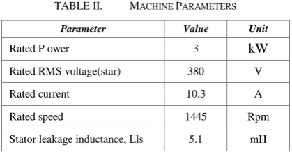
To demonstrate the performance of the control strategy when a motor load is connected to the matrix converter, a 3 kW induction machine is driven by the direct MC at no load. The parameters of the machine are shown in Table. II. The speed of the machine is controlled by a PI controller and the stator current control is achieved by the DPCVC. The machine is initially magnetized and a speed demand of 500 rpm is applied to the system. The resulting waveforms of the speed and d and q-axis stator current tracking their respective references is shown in Fig.17. It is evident from Fig.17 that the stator currents follow their reference values without any steady state error despite the inherent uncertainty in the true machine parameters. In fact, it is well known that the steady state response of predictive control methods depends on accurate load parameters. Nevertheless, given the high equivalent gain of the proposed method, any tracking error produced by parameter mismatch will be small. The THD of the controlled stator currents is 3.7%.
TABLE II. MACHINE PARAMETERS
Parameter Value Unit
Rated P ower 3 kW
Rated RMS voltage(star) 380 V
Rated current 10.3 A
Rated speed 1445 Rpm
Stator leakage inductance, Lls 5.1 mH
0 0.01 0.02 0.03 0.04 0.05
Time (s) -2 -1 0 1 2 T h re e P h s u p p ly c u rr en ts ( A
) Phase A
Phase B Phase C
0.1 0.15 0.2 0.25 0.3 0.35 0.4
-5 0 5 T h re e p h as e lo ad c u rr en ts (A ) Phase A Phase B Phase C
2.2 2.3 2.4 2.5 2.6 2.7 2.8
[image:13.595.193.403.605.715.2]Parameter Value Unit
Rotor leakage inductance, Llr 7.3916 mH
Mutual inductance, L 0.2388 H
Stator resistance, Rs 1.9 Ω
Rotor resistance, Rr 1.33 Ω
[image:14.595.158.440.49.381.2]Supply V oltage, Vs 120 V
Fig 17. Experimental results: Speed and stator currents of an IM controlled by DPCVC
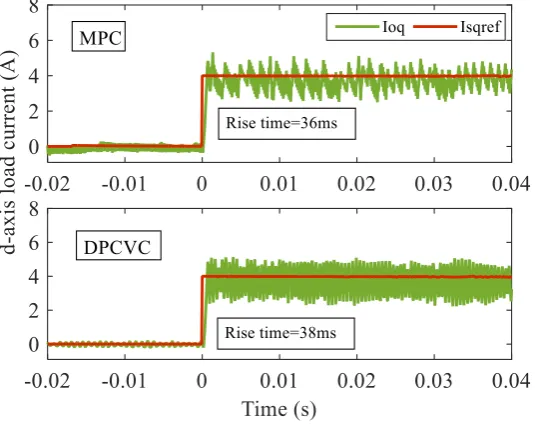
In order to compare the transient behavior of the proposed control strategy with MPC, the step change in the d-axis stator current when driving an IM is considered. The resulting waveforms shown in Fig.18 demonstrates that the rise times of the current when controlled by MPC and DPCVC are 36ms and 38ms respectively. This indicates that DPCVC can achieve a fast dynamic response which is comparable to the conventional MPC, while keeping constant switching frequency and improved supply currents.
[image:14.595.163.431.460.672.2]The control of both supply and load currents of a direct matrix converter are attained by the proposed control method. The experimental results included in this section validate the simulation results and hence proves the control theory. The main objective of this method has been to develop a strategy based on predictive control which results in a fixed switching frequency, delivering good quality waveforms without sacrificing the steady state waveform quality. The proposed method ensures that the inherent characteristic of a predictive based controller such as fast dynamic response is preserved. On the other hand the steady state performance is considerably improved due to the modulation approach included in the method.
VI. CONCLUSIONS
A novel model based predictive control approach for a direct matrix converter that has an inbuilt modulation scheme to control both the input and output side currents is proposed in this paper. The main achievement of this approach is the fusion of predictive control and a modulation method for a direct matrix converter to result in a fixed switching frequency operation while retaining the merits of a predictive based controller such as fast transient response. Under saturation, the method can be modified to prioritize control of input or output currents, although it can just as easily be modified to prioritize control of input currents, depending on the requirements. A comparison of load current control of the proposed control method with MPC is also showcased in this work. Equations for the control of supply side and load side currents were derived using the system model and simulation results and experimental results are included to validate the control theory.
REFERENCES
[1] A. Alesina and M. Venturini, "Analysis and design of optimum-amplitude nine-switch direct AC-AC converters," Power Electronics, IEEE Transactions on, vol. 4, pp. 101-112, 1989.
[2] L. Huber and D. Borojevic, "Space vector modulated three-phase to three-phase matrix converter with input power factor correction," Industry Applications, IEEE Transactions on, vol. 31, pp. 1234-1246, 1995.
[3] D. Casadei, G. Serra, and A. Tani, "The use of matrix converters in direct torque control of induction machines," Industrial Electronics, IEEE Transactions on, vol. 48, pp. 1057-1064, 2001.
[4] R. Vargas, J. Rodriguez, U. Ammann, and P. W. Wheeler, "Predictive Current Control of an Induction Machine Fed by a Matrix Converter With Reactive Power Control," Industrial Electronics, IEEE Transactions on, vol. 55, pp. 4362-4371, 2008.
[5] P. Zanchetta, P. W. Wheeler, J. C. Clare, M. Bland, L. Empringham, and D. Katsis, "Control Design of a Three-Phase Matrix-Converter-Based AC–AC Mobile Utility Power Supply," Industrial Electronics, IEEE Transactions on, vol. 55, pp. 209-217, 2008.
[6] J. Rodriguez, J. Pontt, R. Vargas, P. Lezana, U. Ammann, P. Wheeler, et al., "Predictive direct torque control of an induction motor fed by a matrix converter," in Power Electronics and Applications, 2007 European Conference on, 2007, pp. 1-10.
[7] R. Vargas, U. Ammann, B. Hudoffsky, J. Rodriguez, and P. Wheeler, "Predictive Torque Control of an Induction Machine Fed by a Matrix Converter With Reactive Input Power Control," Power Electronics, IEEE Transactions on, vol. 25, pp. 1426-1438, 2010.
[8] P. Wheeler, J. C. Clare, M. Apap, D. Lampard, S. Pickering, K. J. Bradley, et al., "An Integrated 30kW Matrix Converter based Induction Motor Drive," in Power Electronics Specialists Conference, 2005. PESC '05. IEEE 36th, 2005, pp. 2390-2395.
[9] E. F. Camacho and C. B. Alba, Model predictive control: Springer, 2013.
[10] J. Rodriguez and P. Cortes, "Model Predictive Control," in Predictive Control of Power Converters and Electrical Drives, ed: John Wiley & Sons, Ltd, 2012, pp. 31-39.
[11] L. Tarisciotti, P. Zanchetta, A. Watson, J. Clare, and S. Bifaretti, "Modulated Model Predictive Control for a 7-Level Cascaded H-Bridge back-to-back Converter," Industrial Electronics, IEEE Transactions on, vol. PP, pp. 1-1, 2014. [12] L. Tarisciotti, P. Zanchetta, A. Watson, J. Clare, S. Bifaretti, and M. Rivera, "A new predictive control method for cascaded
multilevel converters with intrinsic modulation scheme," in Industrial Electronics Society, IECON 2013 - 39th Annual Conference of the IEEE, 2013, pp. 5764-5769.
[13] L. Tarisciotti, P. Zanchetta, A. Watson, J. Clare, M. Degano, and S. Bifaretti, "Modulated model predictve control (M<sup>2</sup>PC) for a 3-phase active front-end," in Energy Conversion Congress and Exposition (ECCE), 2013 IEEE, 2013, pp. 1062-1069.
[15] M. Vijayagopal, P. Zanchetta, L. Empringham, L. D. Lillo, L. Tarisciotti, and P. Wheeler, "Modulated model predictive current control for direct matrix converter with fixed switching frequency," in Power Electronics and Applications (EPE'15 ECCE-Europe), 2015 17th European Conference on, 2015, pp. 1-10.
[16] L. Tarisciotti, J. Lei, A. Formentini, A. Trentin, P. Zanchetta, P. Wheeler, et al., "Modulated Predictive Control for Indirect Matrix Converter," IEEE Transactions on Industry Applications, vol. 53, pp. 4644-4654, 2017.
[17] Z. Di, M. Rivera, H. Dan, L. Tarisciotti, K. Zhang, D. Xu, et al., "Modulated model predictive current control of an indirect matrix converter with active damping," in IECON 2017 - 43rd Annual Conference of the IEEE Industrial Electronics Society, 2017, pp. 1313-1318.
[18] M. Vijayagopal, L. Empringham, L. d. Lillo, L. Tarisciotti, P. Zanchetta, and P. Wheeler, "Current control and reactive power minimization of a direct matrix converter induction motor drive with Modulated Model Predictive Control," in 2015 IEEE International Symposium on Predictive Control of Electrical Drives and Power Electronics (PRECEDE), 2015, pp. 103-108.
[19] M. Vijayagopal, P. Zanchetta, L. Empringham, L. d. Lillo, L. Tarisciotti, and P. Wheeler, "Control of a Direct Matrix Converter With Modulated Model-Predictive Control," IEEE Transactions on Industry Applications, vol. 53, pp. 2342-2349, 2017.
[20] E. Fuentes, C. A. Silva, and R. M. Kennel, "MPC Implementation of a Quasi-Time-Optimal Speed Control for a PMSM Drive, With Inner Modulated-FS-MPC Torque Control," IEEE Transactions on Industrial Electronics, vol. 63, pp. 3897-3905, 2016.
[21] M. Apap, J. C. Clare, P. Wheeler, and K. J. Bradley, "Analysis and comparison of AC-AC matrix converter control strategies," in Power Electronics Specialist Conference, 2003. PESC '03. 2003 IEEE 34th Annual, 2003, pp. 1287-1292 vol.3.
[22] D. Casadei, G. Serra, A. Tani, and L. Zarri, "Matrix converter modulation strategies: a new general approach based on space-vector representation of the switch state," Industrial Electronics, IEEE Transactions on, vol. 49, pp. 370-381, 2002. [23] L. Furong, C. Klumpner, and F. Blaabjerg, "Stability analysis and experimental evaluation of a matrix converter drive system," in Industrial Electronics Society, 2003. IECON '03. The 29th Annual Conference of the IEEE, 2003, pp. 2059-2065 Vol.3.