This is a repository copy of Identification of continuous-time models for nonlinear dynamic
systems from discrete data.
White Rose Research Online URL for this paper:
http://eprints.whiterose.ac.uk/103208/
Version: Accepted Version
Article:
Guo, Y., Guo, L.Z., Billings, S.A. et al. (1 more author) (2016) Identification of
continuous-time models for nonlinear dynamic systems from discrete data.
INTERNATIONAL JOURNAL OF SYSTEMS SCIENCE, 47 (12). pp. 3044-3054. ISSN
0020-7721
https://doi.org/10.1080/00207721.2015.1069906
This is an Accepted Manuscript of an article published by Taylor & Francis in International
Journal of Systems Science on 27 July 2016, available online:
http://www.tandfonline.com/10.1080/00207721.2015.1069906.
[email protected] https://eprints.whiterose.ac.uk/
Reuse
Unless indicated otherwise, fulltext items are protected by copyright with all rights reserved. The copyright exception in section 29 of the Copyright, Designs and Patents Act 1988 allows the making of a single copy solely for the purpose of non-commercial research or private study within the limits of fair dealing. The publisher or other rights-holder may allow further reproduction and re-use of this version - refer to the White Rose Research Online record for this item. Where records identify the publisher as the copyright holder, users can verify any specific terms of use on the publisher’s website.
Takedown
If you consider content in White Rose Research Online to be in breach of UK law, please notify us by
1
Identification of Continuous Time Models
for Nonlinear Dynamic Systems from Discrete Data
Revised 26/02/2015 Revised 15/06/2015
Yuzhu Guo1, 2, L.Z. Guo1, 2, S. A. Billings1, 2, and Hua-Liang Wei1, 2
1
Department of Automatic Control and Systems Engineering
The University of Sheffield, Mappin Street, Sheffield, S1 3JD, UK.
2
INSIGNEO Institute for in silico Medicine
The University of Sheffield, Mappin Street, Sheffield, S1 3JD, UK.
e-mail for the corresponding author:
[email protected]
Yuzhu Guo received his B.Sc. degree and M.Sc. degree from Beijing Institute of Technology, Beijing, China, in 2001 and 2004, respectively. He received a doctoral degree in automatic control and systems engineering from the University of Sheffield, UK, in 2009. He is now a researcher in the Centre for Signal Processing and Complex Systems and the Insigneo Institute for in sillico Medicine, University of Sheffield, UK. His research interests include nonlinear system identification, non-linear dynamics, spectral analysis, complex spatio-temporal systems, excitable media, and model order reduction with application to biomedical systems.
Lingzhong Guo received both his BSc and MSc degrees in Mathematics in China and PhD degree in Bristol Robotic Laboratory, the University of the West of England, UK. He is currently a Lecturer in the Department of Automatic Control and Systems Engineering of the University of Sheffield, UK. His research interests include identification and analysis of nonlinear dynamic systems with applications in biomedical system.
Stephen A. Billings is a Professor in the Department of Automatic Control and Systems Engineering, University of Sheffield, UK and leads the Signal Processing and Complex Systems research group. His research interests include system identification and information processing for nonlinear systems, narmax methods, model validation, prediction, spectral analysis, adaptive systems, nonlinear systems analysis and design, neural networks, wavelets, fractals, machine vision, cellular automata, spatio-temporal systems, fMRI and optical imagery of the brain, synthetic biology and related fields.
3
Identification of Continuous Time Models
for Nonlinear Dynamic Systems from Discrete Data
Abstract -- A new iOFR-MF (iterative Orthogonal Forward Regression – Modulating Function) algorithm is proposed to identify continuous time models from noisy data by combining the modulating function method and the iterative orthogonal forward regression (iOFR) algorithm. In the new method, a set of candidate terms, which describe different dynamic relationships among the system states or between the input and output, are first constructed. These terms are then modulated using the modulating function method to generate the data matrix. The iOFR algorithm is next applied to build the relationships between these modulated terms which includes detecting the model structure and estimating the associated parameters. The relationships between the original variables are finally recovered from the model of the modulated terms. Both nonlinear state-space models and a class of higher order nonlinear input-output models are considered. The new direct method is compared with the traditional finite difference method and results show that the new method performs much better than the finite difference method. The new method works well even when the measurements are severely corrupted by noise. The selection of appropriate modulating functions is also discussed.
Key words: Continuous time model, iOFR algorithm, modulating function method, nonlinear system
4
1. Introduction
The system identification of discrete time models has been well developed for both linear and
nonlinear systems. Many different identification methods based on different criterions have been
developed and used (Ljung, 1987; Söderström, 1989; Söderström & Stoica, 2002). Among the existing
nonlinear system identification methods, the NARMAX (Nonlinear AutoRegressive Moving Average
with eXogenous input) model and the associated Orthogonal Forward Regression (OFR) algorithm
have been widely applied in the modelling of many engineering, chemical, biological, medical,
geographical, and economic systems (Billings, 2013). However, a continuous time model is often
favourable in some applications because of the inherent connection with physical systems.
There are essentially two classes of identification methods for continuous time models: the direct
methods and the indirect methods (Unbehauen & Rao, 1998). The direct methods identify
continuous time models directly from discrete data, but this often involves the reconstruction of the
derivatives of variables from the discrete data (Coca & Billings, 1999). A very commonly used
method is the finite difference method, for example, the methods based on the delta operator
models (Anderson & Kadirkamanathan, 2007; Soderstrom, Fan, Carlsson, & Mossberg, 1997; Zhang
& Billings, 2015). However, the numerical differentiation that is inherent in this approach may
amplify the effects of noise, which makes the application of the finite difference impractical in many
applications. The performance of these kinds of direct methods crucially depends on the filters used
in the data pre-processing. Other direct methods include algorithms based on signal decompositions
where the signals are reconstructed using a system of basis functions and the derivatives of the
signals are calculated as the combination of the derivatives of these basis functions (Brewer,
Barenco, Callard, Hubank, & Stark, 2008; Coca & Billings, 1997). To avoid numerical differentiation,
indirect methods have been developed in the identification of continuous time models. These
approaches involve the identification of discrete time models as a first step and then the transfer of
the discrete-time models to continuous time models (Li & Billings, 2001). The transfer is based on
some invariant properties between the discrete and continuous models, for example, the impulse
response, the frequency response functions and so on. Despite the fact that the indirect methods
often give good representations for a physical system, the transformation from discrete model to
continuous model can become complicated when the system is nonlinear.
The modulating function method which directly produces continuous time models avoiding
numerical differentiation of noisy data has been widely used in many applications (Preisig & Rippin,
1993; Saha & Rao, 1983; Unbehauen & Rao, 1990, 1998; Young, 1981). However, the modulating
5 identification method and there are few studies that investigate the model structure detection in
the modulating function method. In many applications, both the model structure and the unknown
parameters need to be determined.
In this paper, a new iOFR- modulating function method is introduced, which combines the strengths
of both the iOFR algorithm and the modulating function method. It will be shown that the model
structure can be efficiently detected by adopting the iOFR algorithm to select the modulated
candidate terms. The iOFR-MF algorithm provides a new and efficient method for identifying
nonlinear continuous time models.
System identification involves two coupled problems: the detection of the model structure and
estimation of the parameters. The detection of the model structure depends on the values of the
associated parameters and the estimation of the parameters depends on the model structure.
Therefore system identification searches for a solution in the Cartesian product of the set of
candidate terms and the set of possible parameters. An exhaustive search on the whole solution
space is often time-consuming and impractical in many applications. Evolutionary algorithms are
often used to reduce the computation of the global search, for example the symbolic regression
algorithms (Koza, 1992; Schmidt & Lipson, 2009). Even the evolutionary algorithms can be
computationally intensive when the solution space is large. The OFR (Orthogonal Forward
Regression) algorithm, which has successively decoupled these two processes by stepwise
orthogonalising the candidate terms and selecting the significant terms one at a time, has been
proved to be efficient in the identification of nonlinear systems. A new iOFR (iterative Orthogonal
Forward Regression) algorithm has recently been proposed to improve the performance of the
classic OFR algorithm (Yuzhu Guo, L.Z. Guo, S. A. Billings, & H. L. Wei, 2015b). In the iOFR algorithm,
the classic OFR algorithm is iteratively applied where the next search is based on the suboptimal
term set obtained at the previous stage. By slightly revising the classic OFR algorithm, the iOFR
algorithm searches an optimal model on a global solution space and produces the optimal solution.
In this paper, the iOFR algorithm will be combined with the modulating function method to provide
a new system identification method where both the system structure can be efficiently detected and
the parameters can be estimated avoiding all the problems caused by numerical differentiation of
noisy data. The new algorithm can efficiently determine a parsimonious model structure without any
a priori knowledge of the nonlinear system.
The remainder of the paper is organised as follows. Section 2 introduces the continuous-time models
6 introduced in Section 3. In Section 4, the Lorenz system and van der Pol oscillator are identified to
demonstrate the efficiency of the new method. Conclusions are finally drawn in Section 5.
2. Continuous models and the modulated representation
The main idea of the modulating function method is to transfer the derivatives of measured, noisy
signals to analytical modulation functions. This transfer is achieved by integrating by parts the
product of the modulating function with the terms in the model equation. A similar idea has also
been used in the finite element method and distribution theory where the modulating function is
referred to as the test function and the modulated equation is named as the weak formulation. In
order to apply the modulating function method, the modulating functions are required to posses
some good properties. The modulating functions are introduced in Section 2.1 and Section 2.2 and
2.3 show how to transform differential equations into algebraic relations between the modulated
terms using these modulating functions.
2.1 Modulating functions
The modulating function is chosen to possess the following properties:
i). The modulating function ϕ( )t has finite support, that is, ϕ( )t is identically zero outside the finite interval [ , ]a b .
ii). The modulating function is sufficiently smooth, that is, the up to d-th derivatives exist.
iii). The derivatives of the modulating function are zero at the ends of the finite interval.
Many functions have been used as modulating functions, including trigonometric functions, the
Poisson moment functions, Hartley functions, and so on. In this paper the B-spline function is used
as the modulating function because of the simple structure and excellent approximation properties
of these functions.
A kth order B-spline function can be recursively defined as follows given a set of k+1 knots s0, s1, …,
1 k
s+ .
( )
( )
( )
, , 1 1, 1
1 1
i i k
i k i k i k
i k i i k i
t s s t
B t B t B t
s s s s
+
− + −
+ − + +
− −
= +
− − (1)
with
( )
1,1
1, 0,
i i
i
s t s
B t
otherwise
+
≤ <
=
7 The first index indicates the position of the B-spline function and the second index denotes the order
of the B-spline functions. Using k+1 knots one kth order B-spline function can be defined and two
(k-1) th order B-spline functions can be defined, in turn, three (k-2)th order B-spline functions, and so
on.
The derivative of a k-th order B-spline can be calculated as
( ) ( )
( )
( )
, , 1 1, 1
1 1
1
i k i k i k
i k i i k i
dB t B t B t
k
dt s s s s
− + −
+ − + +
= − −
− −
(3)
The higher order derivative of a B-spline basis function can be calculated according to the recursive
formula:
( ) ( )
( )
( )
1 , 1
1 ,
1
1 1 1, 1
1
1 1
1
r i k
r r
i k
r r
i k i i k i i k r
d B t
d B t dt
k
s s s s
dt d B t
dt
− − − −
+ − + + + −
−
−
= −
− −
[image:8.595.180.421.286.343.2] [image:8.595.183.402.450.629.2](4)
Figure 1 shows the cubic (4th order) B-spline function and its first and second order derivatives. It is
easy to observe that the B-spline function satisfies all the requirements of a modulating function.
The advantages of the spline function over other modulating functions has been discussed in the
references (Preisig & Rippin, 1993).
Fig 1 Cubic B-spline basis function and its derivatives
8
2.2 State-space models
A state-space model is a canonical form model for both linear and nonlinear systems where the
system can fully be described by a minimum number of state variables. Consider the state-space
model in equation (5).
( ) ( ( ), ( ))
( ) ( ) ( )
t t t
y t x t n t
= = + ɺ
x f x u
(5)
where x t( ) is the state vector of the system; y t( ) is the measurements of the system states x t( ) and
( )
n t is measurement noise. The function f x t u t( ( ), ( )), which can be any linear or nonlinear function
of the system states and inputs, defines a vector field which uniquely determines the transition of
system states in the state space. The vector function f
( )
x u, can often be expanded as the superposition of a set of basis functions, that is.1
( ) ( , )
s i i i
x t x u
κ θ φ
=
=
∑
ɺ (6)
The model then becomes linear-in-the-parameters, and θi represents the system parameters. Multiplying both sides of equation (6) with the modulating function ϕ( )t and integrating both sides over the time interval [a, b] yields
( ) ( )
(
( )
(
( ) ( )
)
)
1 , s b b i i a a ix d x u d
κ
ϕ τ τ τ θ ϕ τ φ τ τ τ
=
=
∑
∫
ɺ∫
(7)The left hand side of the equation can be written as (8) using the rule of integration by parts.
( ) ( )
( ) ( )
( ) ( )
b b b
a
aϕ τ x τ τ ϕd = t x t − aϕ τ x τ τd
∫
ɺ∫
ɺ (8)Because of the properties of the modulation function, the first term on the right hand side is always
zero and the modulated system model becomes
( ) ( )
(
( )
(
( ) ( )
)
)
1 , s b b i i a a ix d x u d
κ
ϕ τ τ τ θ ϕ τ φ τ τ τ
=
−
∫
ɺ =∑
∫
(9)In system identification, modelling is usually performed based on the noisy observations y t( ) rather
than the state variables x t( ). Using the modulating function method, the differentiation operation
on the noisy observations y t( ) are successfully transferred onto the analytic modulating function
( )
tϕ . At the same time, the structure of the model remains unchanged. Therefore, the
9 from the observed input and output data. In practical applications, the form of the function f x u( , )
is often not known a priori, that is, what kind of terms φi( , )x u should be included in the model (6) needs to be determined before parameter estimation. This problem is crucial to the system
identification and has not been well studied in the application of the modulating function method. In
this paper, the iOFR algorithm will be adopted to solve the problem of model structure detection in
the modulation function method. A large candidate term dictionary, in which all the possible terms
are included, will initially be constructed. All these terms will then be modulated using the
modulating function. The most significant terms will be selected from the modulated term dictionary
using the new iOFR algorithm to constitute the system model. The new iOFR-modulating function
method will be discussed in Section 3.
2.3 Higher - order continuous systems
When some of the inner-states in (5) cannot be directly measured the system can be described using the input-output model
(
)
( ) ( 1) ( 2) ( 1) ( 2)
, , , , , , , , ,
n n n n n
y = f y − y − ⋯ y y uɺ − u − ⋯ u uɺ (10)
Here we assume the highest derivative ( )n
y is linear and with a unit coefficient in the model. Actually, the left hand side of the equation can be any linear combination of measurable variables and the associated derivatives. For example, a mechanical system can be written in the form
( )
,myɺɺ+ +cyɺ ky= f y yɺ , where m, c, k represent the mass, damping coefficient, elastic coefficient, respectively, and f y y
( )
ɺ, is the nonlinear restoring force. However, in many applications the form and the nonlinear restoring force is not known and is usually approximated using a series of basis functions.Expanding the function on the right hand side as the superposition of basis terms yields
(
)
( )
1
1
( ) ( 1) ( 2) ( 1) ( 2)
1
, , , , , , , , , ,
s
n n n n n
i i i i
i i
y y y y y u u u u y u
κ κ
κ
θ φ − − − − θ φ
= =
=
∑
⋯ ɺ ⋯ ɺ +∑
(11)It is worth noticing that the modulating function cannot be used in the general input-output model in (11). The modulating function method requires the term
(
( 1) ( 2) ( 1) ( 2))
, , , , , , , , ,
n n n n
i y y y y u u u u
φ − − − −
ɺ ɺ
⋯ ⋯
to be integrable, that is, φi ( i = 1, 2, …,κ1 ) is the derivative of another function ψi
( )
y u, with respected to time, that is,( )
(
( 1) ( 2) ( 1) ( 2))
, , , , , , , , , ,
i
i n
n n n n
i i
n
d
y u y y y y u u u u
dt ψ φ
− − − −
10 Term ψi
( )
y u, can only be a function of the input and output not including their derivatives so thatthe time derivatives of the input and output can be fully transferred on to the analytic modulating function. When all the terms satisfy the requirements, the modulated model can be given as
( )
( ) ( )
( )
( )
(
( ) ( )
)
( ) ( )
(
)
1 1 ( ) ( ) 1 1 1 , i i s b bn n n n
i a a i b i i a i
y d y u d
y u d
κ
κ κ
ϕ τ τ τ θ ϕ τ ψ τ τ τ
θ φ τ τ τ
= = − = − +
∑
∫
∫
∑ ∫
(13)Again, the model structure needs to be detected before the parameters can be estimated based on the modulated model.
2.4 Relationship with the finite difference method
In order to explain why the modulating function method works better than a finite difference method, the relationship between the finite difference method and the modulating function method will be discussed. It will be shown that the finite difference method is a specialisation of the modulating function method where the modulating function is the second order B-spline function.
Assume the data is uniformly sampled with the sampling interval ∆t and the continuous signal can be constructed using a zero-order hold, that is,
( ) (
1 ,)
1x t =x k− k− ≤ <t k (14)
The finite difference formulae
( )
x k( ) (
x k 1)
x k
t
− −
≈
∆
ɺ (15)
can then be thought as the modulated form of the following modulating function.
( )
( )
( )
2 2 ( 1) 1 ( 1) 1 t kk t k
t t
k t
k t k
t
ϕ
− −
− ≤ <
∆
=
+ −
≤ < +
∆
(16)
The derivative of ϕ
( )
t is( )
( )
( )
2 2 1 1 1 1k t k
t t
k t k
t
ϕ
− ≤ <
∆
=
− ≤ < + ∆
ɺ (17)
Compare the modulating function in (16) and (17) with formulae (1) and (3). It is easy to see that
modulating function (16) is similar to the second order B-spline function where the three knots used
11 function method where the modulating function is defined as (16) and the derivative is (17).
However, the second order B-spline function with the finite support [k-1, k+1] is not a good choice
for the modulating function and the estimated parameters are often not satisfactory. How to choose
an appropriate modulating function will be discussed in the next section.
3. Iterative orthogonal forward regression modulating function
method
When the structure of the differential equation models are known, the differential equations can be
transformed into algebraic equations with the structure of the equation unchanged using the
modulating function. The associated parameters can then be estimated without any numerical
differentiation. However, the structure of the model is often unknown. Hence a system identification
method which can identify both the model structure and the associated parameters is needed. In
this section a new iterative orthogonal forward regression modulating function method is
introduced by combining the modulating function method with the iterative orthogonal forward
regression algorithm.
3.1 Application of the iterative orthogonal forward regression algorithm in
the modulating function method
In order to determine the model structure, a term dictionary D =
{
φ1,⋯,φκ}
is initially defined andthe model to be identifed is assumed to be composed of a linear combination of a subset of the
terms in the dictionary. To apply the iOFR algorithm, the dependent variable and these terms will be
modulated first and these modulated candidate terms are then used to construct the modulated
regression matrix.
In the previous section, only one set of data was generated through the integration over the support
of the modulating function. In order to identify the modulated model, more data are needed.
Additional data for the modulated model can be generated in two ways: shifting the position of the
modulating function over the signals or alternatively, using different modulating functions. Either
way, different modulating functions, which can be different in the form of function or different in
the interval of support, are obtained. Define these modulating functions as ϕk
( )
t , k=1,2,…, N, and denote the associated nth order derivative as ( )n( )
k t
ϕ .
Collecting N sets of the modulated terms yields the matrix form of equation
12 where Y=[y(1), y(2), …, y(N)], and
( ) ( )
( )( ) ( )
1n b kn
a
y k = −
∫
ϕ τ y τ τd . Matrix Φ=[
φ φ1 2 ⋯ φκ]
isknown as the modulated regression matrix. Each column φi =
[
ηi(1) ⋯ ηi( )N]
T represents Nrealization of a modulated term.
When the original term does not contain the derivatives of the input or output, the corresponding modulated term of φi
(
y( ) ( )
τ ,u τ)
is( )
( )( )
(
( ) ( )
)
,
i b
n
i k a k i y u d
η =
∫
ϕ τ φ τ τ τ (19)Otherwise, the modulated term will be
( ) ( )
( )( )
(
( ) ( )
)
1 ni b ni
i k a k i y u d
η = −
∫
ϕ τ ψ τ τ τ (20)when the original term also depends on the derivatives of the input or output, where ψi
(
y( ) ( )
τ u τ)
is defined in (12).
However, which terms should be included in a model is often unknown a priori. Hence, system
identification involves the determination of the model structure which consists of a subset
{ }
φj of the term in the dictionary D ={
φ1,⋯,φk}
and the estimation of the associated parameters. Thesetwo processes are firmly coupled with each other. Ranking of the significance of a term depends on
the weight (coefficient) of the term in a model while the estimation of the parameters depends on
what terms are included in a model. The OFR algorithm decouples the interactions between these
two processes and provides an efficient method for the identification of nonlinear systems. In the
OFR algorithm, the terms φj are orthogonalised stepwise into the orthogonal terms wj and the associated coefficients can then be estimated as
, ,
j j
j j
w y g
w w
= (21)
The significance of the term can then be evaluated using the Error Reduction Ratio or ERR criterion
defined as
( )
, , 2, , ,
j j j j j j
j j
g w g w w y
ERR w
y y w w y y
= = (22)
13 The regression will stop when all the significant terms have been detected. A commonly used stop
condition can be set as
( )
1 j
j
ERR w ρ
−
∑
≤ (23)The sum of ERR (denoted as SERR) indicates that a proportion of
( )
jj
ERR w
∑
information in theoutput has been explained by the terms { }φj which consists the model.
The standard orthogonal forward regression algorithm consists of the following steps:
(1) Sufficiently excite the system and measure the inputs and outputs of the system.
(2) Specify an initial full model set of κcandidate terms and the value of ρ .
(3) Compute the values of the ERR for each of the κ candidate terms and select the term which
gives the largest value of ERR into the model as the first term.
(4) At the kth (k≥2 ) stages: compute the values of the error reduction ratio for each of the
(κ − +k 1) remaining candidate terms by assuming that each is the kth term in the selected model and perform the corresponding orthogonalisation; the term that gives the largest value of the error
reduction ratio is then selected into the model as the kth term. If condition (23) is satisfied, finish
the process and go to (5). Otherwise set k= +k 1 and repeat step (4).
(5) The final model contains κs terms and the parameter estimates can be calculated using a least
squares formulae.
The classic OFR algorithm can occasionally produce sub-optimal models, for example, when the
system is not persistently excited. An iterative OFR (iOFR) algorithm has recently been introduced to
solve this problem. The iOFR algorithm comprises two steps, the first step is to obtain a suboptimal
model set and the second step uses a subset of the terms which were obtained in the first step as
the starting point of a global search. The new iterative OFR algorithm can be summarised in the
following steps.
i) Preset a tolerance ρ and apply the standard OFR algorithm on the whole term dictionary Φ to produce a suboptimal term set
{
}
1 2 s
s = s s sκ
Φ φ φ ⋯ φ ;
14 iii) Select a subset Φpre⊂Φs of the terms φj, where j=s s1, 2,⋯,sκs, in Φs as preselected terms and
search the other terms on the term set Φ Φ\ pre to construct a suboptimal solution satisfying
1−
∑
ERRi < + ∆ρ ρ;iv) Repeat iii) for different subset Φpre’s of Φs and obtain some suboptimal models;
v) Compare the obtained suboptimal models and choose the best one as the final model Φop .
Remarks:
The subset Φpre is often selected as a combination of p terms in Φs. There are a total number of
( )
s pκ combinations. All the combinations are evaluated in step iv) and
( )
s pκ candidate models are
obtained. However, in most cases, the new iOFR can produce the optimal model using the setting
p=1 (Yuzhu Guo, L. Z. Guo, S. A. Billings, & H. L. Wei, 2015a).
3.2 Selection of appropriate modulating functions
Using the B-spline form modulating functions three parameters need to be determined before the
application of the OFR-modulating function method: the order of the B-spline function k, the length
of the support interval (b-a) of the modulating function, and the shift time with which the
modulating functions are sliding over the signal.
A kth order B-spline function is (k-1) times differentiable. Hence, in order to identify an mth order
dynamic system, at least an (m+1)th B-spline function is needed. When the modulating function
smoothly slides over the signal, the modulating process is actually a convolution of the modulating
function and the signal. From the frequency domain viewpoint, the modulating function acts as a
filter of which the impulse response function is the modulating function. The frequency response
functions of the modulating function and the associated derivatives have been discussed in the
reference where the length of the support interval (b-a) is suggested to take a value of the
dominating time constant of the signal(Preisig & Rippin, 1993). Actually a modulating function with a
smaller support interval which means a wider pass band may keep more information of the original
system in the transformed data but the elimination of the noise will be less significant. Fortunately,
the frequency of noise is often much higher than the system frequencies. The selection of the sliding
interval is relatively flexible, which depends on the number of the data available and the number of
data needed for parameter estimation. A very small sliding interval time may cause the modulated
15
4. Test examples
In this section, the Lorenz system and the van der Pol oscillator will be used to show the efficiency of
the iOFR-MF method. Because of the fact that both examples are autonomous systems, no inputs
can be designed to guarantee the persistent excitation of the systems. Some of the system
characteristics may therefore not be fully exhibited in the observed data. For this reason, the
iterative OFR algorithm is used to avoid any potential problems caused by non-persistent excitation
(Guo et al., 2015a). Notice that in both examples we make no assumptions about the form of the
model, the model structure and the unknown parameters are all determined from the data with no
a priori information to simulate the conditions that would exist in the identification of real systems.
4.1 Identification of a Lorenz system
The Lorenz system is widely used as the prototype for the study of chaos. The Lorenz system can be represented using the following nonlinear state-space equations.
(
)
(
)
1
2 1
2
1 3 2
3
1 2 3
dx
x x
dt dx
x x x
dt dx
x x x
dt
σ
ρ
β
= −
= − −
= −
(24)
The parameters are set as σ =10, ρ =28, and β =8/3. The system exhibits chaotic behaviour for these parameters. The system was simulated with a sampling time of 0.002s. In this example, we
assume all the system states are measurable. The simulated data were corrupted by 10% Gaussian
white noise to mimic the effects of measurement noise, that is,
( ) ( ) ( ) 1, 2, 3
i i i
z t =x t +n t i= (25)
where n ti
( )
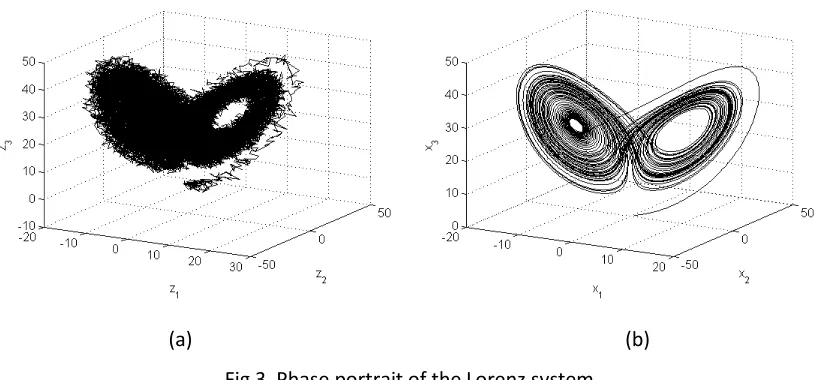
is a Gaussian white noise process.The noisy data are show in Fig 2. Figure 3(a) shows the phase portrait of the noisy data in the
16 Fig 2 Data used for the system identification of the Lorenz system
(a) (b)
Fig 3 Phase portrait of the Lorenz system
(a) Measurement of data (b) Model prediction output of identified model in Table 3
In this example, we assume the relationships among the three variables are not known. Both the
finite difference method and the new iOFR-MF method will be used discover both the nonlinear
interactions among the system states and also the associated parameters. The Lorenz system was
firstly identified using the finite difference method where the derivatives of the system states were
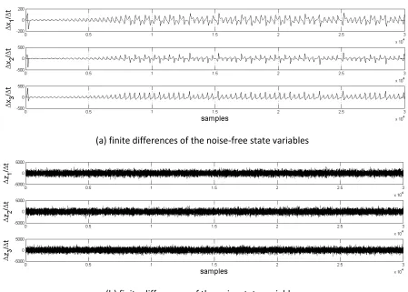
approximated using the finite difference method. The finite differences of the measured states with
10% measurement noise are shown in Fig 4(b). Figure 4(a) shows the finite differences of the
noise-free signals. It can be observed that the useful information in Figure 4(a) is overwhelmed by the
[image:17.595.93.501.246.436.2]17 (a) finite differences of the noise-free state variables
[image:18.595.75.524.73.394.2](b) finite differences of the noisy state variables Fig 4 The finite difference of the system state variables
The model structures were assumed unknown a priori and a term dictionary which consisted of all
the up to third order polynomial terms of the system states was used, that is,
{
2 2 2 3 2 2 2 2 2 2 3}
1, 2, 3, 1, 1 2, 1 3, 2, 2 3, 3, 1, 1 2, 1 3, 1 2, 1 2 3, 1 3, 2 3, 2 3, 3
z z z z z z z z z z z z z z z z z z z z z z z z z z z z z
D = . The significant terms
were selected from the dictionary to form the models using the iOFR algorithm. The identified
results are shown in Table 2. It can be observed that the model structures have been correctly
detected by the iOFR algorithm even through the finite differences of the signals have been severely
corrupted by the noise.However, the parameters are far from the real values.
Table 2 Model identified using the finite difference method for example 1
No. Terms ERRs Coefficients Standard
Deviation
su
b
sy
st
e
m
1 1
2
z 0.058907 35.1577 0.9219
2 z1 5.319224 -42.2815 1.033
SERR -- 5.38 -- --
su
b
sy
st
e
m
2 1 z2 0.615734 -47.6721 1.225
[image:18.595.126.471.638.758.2]18
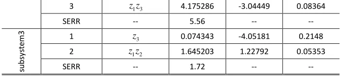
3 z z1 3 4.175286 -3.04449 0.08364
SERR -- 5.56 -- --
su b sy st e m 3 1 3
z 0.074343 -4.05181 0.2148
2 z z1 2 1.645203 1.22792 0.05353
SERR -- 1.72 -- --
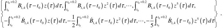
The iOFR-modulating function method was then used to identify the system models where the cubic
(4th order) B-spline function was used as the modulating functions with the length of support of 0.2s.
The modulated derivatives zɺi become 0
(
) ( )
00.2
1,4 0 t
i t B τ t z τ τd
+
−
∫
ɺ − , where t0 represnets the time-shiftof the cubical B-spline function. The dictionary of the modulated terms become
(
) ( )
(
) ( )
(
) ( )
(
)
( )
(
) ( )
0 0 0
0 0 0
0 0
0 0
0.2 0.2 0.2
1,4 0 1 1,4 0 2 1,4 0 3
0.2 2 0.2 3
1,4 0 2 3 1,4 0 3
, , ,...,
,
t t t
t t t
t t
t t
B t z d B t z d B t z d
B t z z d B t z d
τ τ τ τ τ τ τ τ τ
τ τ τ τ τ τ
+ + + + + − − − − −
∫
∫
∫
∫
∫
D =Changing t0and collecting the data yields the data matrix Φ. The iOFR is then appliend and the
identified models are shown in Table 3. The correct model structures have again been successfully
[image:19.595.122.473.74.155.2]identified and now the estimated parameters are very close to the correct values.
Table 3 Results produced by the iOFR-MF method for example 1
No. Terms ERRs Coefficients Standard
Deviation su b sy st e m 1 1 2
z 19.6571 9.9502 0.00753
2 z1 78.65796 - 9.94434 0.008413
SERR -- 98.32 -- --
su b sy st e m
2 1 z z1 3 29.37048 - 0.997504 0.000732
2 z1 69.72317 27.9166 0.03067
3 z2 0.191828 - 0.973564 0.01086
SERR -- 99.29 -- --
su b sy st e m 3 1 1 2
z z 53.07191 1.0024 0.000381
2 z3 46.49793 - 2.67029 0.001485
SERR -- 99.57 -- --
4.2 Identification of a van der Pol oscillator
In this example, the van der Pol oscillator (26) will be identified to illustrate the identification of
higher order input-output models. The van der Pol oscillator is widely used in the study of the limit
19
(
)
( ) ( ) ( )
2
2
2 1 0
d x dx
x x
dt dt
z t x t n t
µ − − + = = + (26)
The coefficient of the nonlinear damping was set as µ =3 and the period of the stable limit cycle is about 7.7s. The van der Pol oscillator was simulated using the 4th order Runge-Kutta algorithm at a
sampling interval 0.01s and 10% Gaussian noise is added to the signal as the measurement noise.
This time, only the displacement x t( ) of the system is observed. The new iOFR-MF method is
employed to identify the nonlinear relationship between the displacement, velocity and the
acceleration. The structure of the system model is assumed unknown and assumed to have the form
in (11). The left hand side of the equation was selected as the second order derivative ɺɺx of the
system state with respect to time. The iOFR-modulating function method is used to detect the
structure of the right hand side of the equation. The initial term dictionary was composed of the up
to 5th order integrable polynomial terms
{
2 3 4 5 2 3 4}
, , , , , , , , ,
z z z z z z zz z z z z z zɺ ɺ ɺ ɺ ɺ . Obviously, more other
intergrable terms can be included in the dictionary, for example sin x x
( )
ɺ. All the terms in the dictionary were modulated by a cubical B-spline function with a finite support 2s. The modulatedterms are
(
) ( )
(
) ( )
(
) ( )
(
) ( )
(
) ( )
(
) ( )
0 0 0
0 0 0
0 0 0
0 0 0
0.2 0.2 0.2
2 5
1,4 0 1,4 0 1,4 0
0.2 0.2 0.2
2 5
1,4 0 1,4 0 1,4 0
, , , ,
1 1
, , ,
2 5
t t t
t t t
t t t
t t t
B t z d B t z d B t z d
B t z d B t z d B t z d
τ τ τ τ τ τ τ τ τ
τ τ τ τ τ τ τ τ τ
+ + + + + + − − − − − − − − −
∫
∫
∫
∫
∫
∫
⋯ɺ ɺ ⋯ ɺ
.
Change the time-shift t0 and construct the data matrix Φ. The system was then identified using the
iOFR-modulating function method and the results are shown in Table 3. It can be observed that all
[image:20.595.109.490.429.477.2]the correct terms are selected and the associated coefficients are very close to the real values.
Table 3 Results produced by the iOFR-MF algorithm for example 2
No. Terms ERRs Coefficients Standard
Deviation
1 x 39.53174 -0.9966 0.00112
2 2
x xɺ 13.23519 -2.00579 0.002159
3 xɺ 46.89805 2.0219 0.002464
20
5. Conclusions
Although the modulating method has been widely used for the identification of continuous models
since it was introduced in 1954 (Shinbrot), the crucial problem about model structure detection has
not been studied. In this paper, an efficient iOFR algorithm is used to extend the modulating
function method to determine the correct model structure. A new iOFR-modulating function method
is proposed to identify continuous time models direct from discrete data, involving both model
structure detection and the associated parameter estimation. Simulations showed that the new
algorithm performs significantly better than the finite difference method especially when the data is
seriously polluted by noise.
Acknowledgements
The authors gratefully acknowledge support from the UK Engineering and Physical Sciences Research
Council (EPSRC) and the European Research Council (ERC).
References
Anderson, S. R., & Kadirkamanathan, V. (2007). Modelling and identification of non-linear deterministic systems in the delta-domain. Automatica, 43(11), 1859-1868. doi:
http://dx.doi.org/10.1016/j.automatica.2007.03.020
Billings, S. A. (2013). Nonlinear system identification : NARMAX methods in the time, frequency, and spatio-temporal domains. Hoboken, New Jersey: John Wiley & Sons Ltd.
Brewer, D., Barenco, M., Callard, R., Hubank, M., & Stark, J. (2008). Fitting ordinary differential equations to short time course data (Vol. 366).
Coca, D., & Billings, S. A. (1997). Continuous-time system identification for linear and nonlinear systems using wavelet decompositions. International Journal of Bifurcation and Chaos in Applied Sciences and Engineering, 7(1), 87-96.
Coca, D., & Billings, S. A. (1999). A direct approach to identification of nonlinear differential models from discrete data. Mechanical Systems and Signal Processing, 13(5), 739-755.
Guo, Y., Guo, L. Z., Billings, S. A., & Wei, H. L. (2015a). Identification of linear systems with non-persistent excitation using an iterative forward orthogonal least squares regression
algorithm. International Journal of Modelling, Identification and Control, 23(1), 1-7. Guo, Y., Guo, L. Z., Billings, S. A., & Wei, H. L. (2015b). An iterative orthogonal forward regression
algorithm. Intern. J. Syst. Sci., 46(5), 776-789. doi: 10.1080/00207721.2014.981237 Koza, J. R. (1992). Genetic programming: on the programming of computers by means of natural
selection: MIT Press.
Li, L. M., & Billings, S. A. (2001). Continuous time non-linear system identification in the frequency domain. International Journal of Control, 74(11), 1052-1061. doi:
10.1080/00207170110052239
Ljung, L. (1987). System Identification: Theory for the User. Englewood Cliffs, N.J.: Prentice-Hall, Inc. Preisig, H. A., & Rippin, D. W. T. (1993). Theory and application of the modulating function method - I.
21
Computers & Chemical Engineering, 17(1), 1-16. doi: http://dx.doi.org/10.1016/0098-1354(93)80001-4
Saha, D. C., & Rao, G. P. (1983). Identification of continuous dynamical systems : the poisson moment functional approach. Berlin: Springer-Verlag.
Schmidt, M., & Lipson, H. (2009). Distilling Free-Form Natural Laws from Experimental Data. Science, 324(5923), 81-85. doi: 10.1126/science.1165893
Shinbrot, N. (1954). On the analysis of linear and nonlinear dynamical systems from transient-response data National Advisory Commitee for Aeronautics Technical note 3288 (pp. 1-51). Washington: Ames Aeronautical laboratory, CA.
Söderström, T. (1989). System Identification. New York; London: Prentice Hall.
Soderstrom, T., Fan, H., Carlsson, B., & Mossberg, M. (1997, 10-12 Dec 1997). Some approaches on how to use the delta operator when identifying continuous-time processes. Paper presented at the Decision and Control, 1997., Proceedings of the 36th IEEE Conference on.
Söderström, T., & Stoica, P. (2002). Instrumental variable methods for system identification. Circuits, Systems and Signal Processing, 21(1), 1-9. doi: 10.1007/bf01211647
Unbehauen, H., & Rao, G. P. (1990). Continuous-time approaches to system identification - A survey.
Automatica, 26(1), 23-35.
Unbehauen, H., & Rao, G. P. (1998). A review of identification in continuous-time systems. Annual Reviews in Control, 22(0), 145-171.
Young, P. (1981). Parameter estimation for continuous-time models a survey. Automatica, 17(1), 23-39.