A quantum probability framework for human probabilistic inference

City, University of London Institutional Repository

Citation

:

This is the accepted version of the paper.

This version of the publication may differ from the final published

version.

Permanent repository link:

Link to published version

:

Copyright and reuse:

City Research Online aims to make research

outputs of City, University of London available to a wider audience.

Copyright and Moral Rights remain with the author(s) and/or copyright

holders. URLs from City Research Online may be freely distributed and

linked to.

Running head: A QUANTUM FRAMEWORK FOR PROBABILISTIC INFERENCE

A Quantum Probability Framework for Human Probabilistic Inference

Jennifer S. Trueblood Vanderbilt University

James M. Yearsley Vanderbilt University

Emmanuel M. Pothos City University London

Corresponding Author: Jennifer Trueblood

Department of Psychology Vanderbilt University PMB 407817

2301 Vanderbilt Place Nashville, TN 37240-7817

Abstract

There is considerable variety in human inference (e.g., a doctor inferring the presence of a disease, a juror inferring the guilt of a defendant, or someone inferring future weight loss based on diet and exercise). As such, people display a wide range of behaviors when making inference judgments. Sometimes, people’s judgments appear Bayesian (i.e., normative), but in other cases, judgments deviate from the normative prescription of classical probability theory. How can we combine both Bayesian and non-Bayesian influences in a principled way? We propose a unified explanation of human inference using quantum probability theory. In our approach, we postulate a hierarchy of mental representations, from ‘fully’ quantum to ‘fully’ classical, which could be adopted in different situations. In our hierarchy of models, moving from the lowest level to the highest involves changing assumptions aboutcompatibility(i.e., how joint events are represented). Using results from three experiments, we show that our modeling approach explains five key phenomena in human inference including order effects, reciprocity (i.e., the inverse fallacy), memorylessness, violations of the Markov condition, and anti-discounting. As far as we are aware, no existing theory or model can explain all five phenomena. We also explore transitions in our hierarchy, examining how representations change from more quantum to more classical. We show that classical representations provide a better account of data as individuals gain familiarity with a task. We also show that representations vary between individuals, in a way that relates to a simple measure of cognitive style, the Cognitive Reflection Test.

A Quantum Probability Framework for Human Probabilistic Inference

Everyday we face situations where we must make inferences about the world around us. For example, a doctor must determine the likelihood that a patient has a disease based on a set of symptoms. A juror must decide the probability that a defendant is guilty after hearing the cases made by the prosecution and defense. Or, maybe you want to judge the likelihood that you will weigh less next month if you start exercising more regularly and you improve your diet. In general, the inference problem involves judging the likelihood of some hypothesis (e.g., presence of a disease, guilt of a defendant, future weight loss) based on a series of evidence (e.g., medical symptoms, prosecution and defense cases, changes in your diet and exercise).

Bayesian inference is widely accepted as the normative approach to inference. However, decades of research in human judgment and decision-making have suggested that people’s

judgments often violate the rules of Bayesian inference and classical probability theory (Tversky & Kahneman, 1975). Despite this large literature, there is growing interest in which aspects of human judgment are consistent with normative prescriptions.

One can argue that the strongest empirical evidence for Bayesian principles in human inference comes from the domain of causal reasoning. Causal graphical models (CGMs) or models based on causal Bayes nets have been successful at explaining and predicting a wide range of behavior in causal inference. In a CGM, variables are represented as nodes and directed edges between nodes capture causal relations. These models represent causal relationships using Bayes’ calculus (Kim & Pearl, 1983; Pearl, 1988) with additional assumptions for how interventions work and are considered to provide a normative account of causal judgment. CGMs have been shown to provide distinct predictions for causal inferences driven by observational, intervention-based, and counterfactual situations (Hagmayer, Sloman, Lagnado, & Waldmann, 2007). There are also various models built using this and similar frameworks that account for causal learning,

experience based learning), or learning from statistical or contingency information.

In spite of the success of CGMs, some recent empirical studies report violations of the predictions of these models. For example, all Bayesian networks must satisfy a condition called the Markov property (this property is part of the definition of a Bayesian network; Russell & Norvig, 2003). This condition states that any node in a Bayesian network is conditionally independent of its nondescendents (e.g., noneffects), given its parents (e.g., direct causes). Informally, if we know about the causes of some eventX, then the descendants ofXmay give us information aboutX, but the non-descendants cannot give us any more information aboutX. Recently, various studies (Rottman & Hastie, 2016, 2014; Park & Sloman, 2013; Rehder, 2014; Fernbach & Sloman, 2009; Waldmann, Cheng, Hagmayer, & Blaisdell, 2008; Hagmayer & Waldmann, 2002) have provided evidence that people often violate the Markov condition when making causal inferences.

In another line of research, there has been an attempt to modify existing Bayesian models to explain away erroneous judgments (Costello, 2009; Costello & Watts, 2014). These models are interesting both from a philosophical point of view, because they may shed light on the principles underlying human reasoning, and also from a practical point of view, as an understanding of why we make judgment errors may inform strategies to improve decision making. Despite the promises of these approaches, they are currently limited in scope. The models developed are typically limited to a single judgment fallacy (such as the conjunction fallacy) and as far as we are aware, none of these approaches have been applied to inference directly (which ultimately involves judgments about a hypothesis given a sequence of observations).

We feel that there is a need for a comprehensive modeling framework that can account for a large range of empirical findings. It is clearly the case that both normative Bayesian and

probability models represent one class of models in our hierarchy. The models in the hierarchy vary in the degree to which the representations are classical versus quantum, which is associated with the dimensionality of the model. High dimensional models (which involve more events represented according to classical probability theory) correspond to more complex mental representations whereas lower dimensional models represent simpler mental representations. The transition from one model to another in the hierarchy is effected through changing certain key assumptions, which in turn guides requirements for representation (this is the assumption of

compatibility, which we will extensively consider shortly). The specific mental representation adopted for a problem might depend on a number of factors including task requirements, the complexity of the problem, experience, familiarity, and an individual’s style of cognitive processing (we will focus on the latter two factors in this paper).

Quantum probability theory is the noncommutative analog of classical probability theory derived from quantum mechanics. As formalized by von Neumann (1932), quantum probability theory is a geometric approach to probability where events are represented assubspacesof a Hilbert space1(essentially a vector space). Note that we use the mathematical formalism of quantum theory without the associated physical meaning. In addition, we assume a fully classical neural substrate. By modeling events as subspaces rather than subsets, quantum probability theory entails a different logic than classical probability theory. The logic of quantum probability theory is the logic of subspaces which relaxes some of the assumptions of Boolean logic. In particular, quantum probability theory does not always have to obey the closure, commutative, and

distributive properties.

“impoverished” mental representations, which can be accounted for by quantum probabilities). Quantum cognition is presently best seen as a descriptive, formal theory for how wedoreason under uncertainty, not how weshouldreason. A more detailed discussion of the explanatory scope of quantum models is provided in the General Discussion section.

Quantum cognitive models are typically employed for results that have so far been explained primarily on the basis of individual heuristics. Such models have been able to account for

numerous findings in cognition and decision-making. These include violations of the sure thing principle (Pothos & Busemeyer, 2009), conjunction and disjunction fallacies (Busemeyer, Pothos, Franco, & Trueblood, 2011; Busemeyer, Wang, Pothos, & Trueblood, 2015), interference effects in perception (Conte, Khrennikov, Todarello, Federici, & Zbilut, 2009), violations of dynamic

consistency (Busemeyer, Wang, & Trueblood, 2012), conceptual combinations (Aerts, Gabora, & Sozzo, 2013), interference effects of choice on confidence judgments (Kvam, Pleskac, Yu, & Busemeyer, 2015), the Ellsberg paradox (Haven & Sozzo, in press), and order effects in survey questions (Wang & Busemeyer, 2013). Research has also examined the mechanistic foundations of quantum probability models of cognition (Fuss & Navarro, 2013), showing how complex

(classical) cognitive architectures can give rise to behavior that is best described in terms of quantum theory. Even though quantum cognitive models are descriptive, they typically allow novel predictions (arguably more so than heuristic accounts) and novel insights about the relevant psychological principles.

events, associated with quantum models, should be preferentially used for decisions executed spontaneously with little conscious deliberation.

Compatible events are ones that may be assigned a simultaneous truth value. Thus, if event

X and eventY are compatible, their conjunctionX∧Y is well defined. The probabilities for compatible events obey the Kolmogorov axioms. Two immediate consequences are that for compatible eventsX andY we have,

p(X∧Y) =p(Y∧X),

p(X|Y) =p(Y|X)p(X)

p(Y)

(1)

Almost all events that we encounter in everyday life can in principle be represented in a compatible way. However doing so requires that decision makers have access to the joint

probabilities of all of these events. This may be unfeasible, for example, from the point of view of memory capacity, since the number of probabilities grows exponentially with the number of events being considered. Equally, these probabilities might be difficult to compute, since joint

probabilities correspond to subsets of the sample space. If it takes a finite number of previous experiences to learn the approximate measure of each subset, then the amount of experience required to compute a joint probability again grows exponentially with the number of events considered. For example, consider a situation where there are three binary events,X,Y, andZ, with values 1 or 2. The elementary events arise from the intersection of these three events and include events such asX1∧Y1∧Z2. This sample space has 23=8 elementary events. As the

not get a pay raise’) and the ability to assign coherent subjective probabilities to these events. In contrast with compatible events, incompatible ones are those for whichX∧Y is undefined. Thus although the probabilitiesp(X)andp(Y)exist, the jointp(X∧Y)may not. Typically one can define a modified version of conjunction with an explicit ordering, e.g.X∧Y is taken to meanX and then Y for incompatible variables. This implies thatp(X∧Y)6=p(Y∧X). Because joint events do not exist when events are incompatible, a lower dimensional space can be used to represent them. For example, if three binary eventsX,Y, andZare all incompatible, then they can (minimally) be represented in a two dimensional space.

In quantum models, one can choose to model two events as either compatible or

incompatible. If all events are chosen to be compatible one recovers a classical model, while if no two events are compatible (except for the trivial case of an event and its negation) then one has a maximally quantum model. If there are more than two possible events then there can be

intermediate representations where some subset of events are compatible. Thus we should more accurately speak of a hierarchy of different representations, from fully quantum to fully classical. Note that we use the term ‘hierarchy’ in the colloquial sense because our models can be roughly ordered by dimensionality. However, the models in our ‘hierarchy’ are not nested.

We begin by describing how quantum probability theory gives rise to a hierarchy of mental representations for human inference. In the subsequent sections, we will discuss how our modeling approach explains a number of phenomena in human inference including order effects, reciprocity (i.e., the inverse fallacy), memorylessness, violations of the Markov condition, and

A hierarchy of mental representations

Previously, many researchers have dealt with violations of the rules of classical probability theory, by elaborating rational models through the inclusion of extra assumptions (Costello, 2009; Costello & Watts, 2014) or by rejecting the applicability of classical probability theory wholesale and instead pursuing explanations based on heuristics (Tentori, Crupi, & Russo, 2013). For example, in the domain of causal inference, when behavior violates the rules of CGMs, such as the Markov condition, researchers have elaborated basic networks through the inclusion of hidden variables, which are causally related to all the observed variables and possibly arise from

participants’ general assumptions regarding the relevant stimuli. While these models often provide good accounts of data, the addition of hidden variables is often post hoc, included when a basic CGM fails to capture data. Also, it is sometimes difficult to reconcile hidden variable approaches with empirical data. For example, Rehder (2014) reported results that normative violations were equally likely in domains of economics, meteorology, and sociology as in an abstract (blank) domain. The assumption of hidden variables in a blank domain is unlikely, as such hidden variables are typically motivated from background knowledge considerations. Further, complex CGMs with multiple hidden variables are often difficult to conclusively test.

Rather than elaborating an existing classical model, we expand the range of probabilistic representations relevant in inference judgments. In all rational models, probabilistic inference follows the rules of classical probability theory. We relax this assumption and use quantum probability theory to build a hierarchy of models. Then, depending on the representation (and we will outline specific prescriptions for determining the appropriate representations), probabilistic calculations can be fully classical or demonstrate some of the peculiarities of quantum probability theory. That is, the approach can accommodate both Bayesian predictions and corresponding non-Bayesian deviations (in the specific way, allowed by quantum theory).

dimensionality with the highest dimensional model being fully classical and the lowest dimensional model being fully quantum. Mathematically, models with lower dimensionality involve more incompatible events than models with higher dimensionality. It is in this way that one could consider lower levels in the hierarchy as “more” quantum and higher levels in the hierarchy as “more” classical.

In this paper, we focus on an inference situation involving three binary variables,X,Y, and

E, whereX andY are causes that independently influence an effectE. For example,E might be ‘future weight loss’ andX andY represent diet and exercise. We decided to focus on this situation (also known as a common effect situation) because it is particularly common in everyday causal inference and has been extensively studied in the lab. It has also figured prominently in the development of models of causal reasoning (Griffiths & Tenenbaum, 2005; Cheng, 1997). Further, many of the effects we are interested in can be explored in this situation, without loss of generality. It also allows us a greater degree of comparability across different experiments, which is useful for detailed model analyses. Note that even though we concentrate our efforts on this particular situation, the modeling approach scales to a wider range of inference problems (including problems with more variables that have more than two outcomes).

2-dimensional model

Consider the situation where someone is trying to judge his or her future weight loss. LetE

represent the question “Will I weigh less next month?” with two possible answers{E₁,E2}. That

is, the answer can either be ‘true’ (E1) or ‘false’ (E2). In classical probability theory, we have a

sample spaceScontaining the elementsE1andE2. Since there are only two elements in our

classical sample spaceS, the size ofSis two.

Alternatively, with quantum probability theory, we can represent the very same event ‘weight loss’, with its possible outcomesE₁andE₂, in a multidimensional Hilbert space. To do so, we replace the sample spaceSwith a Hilbert spaceHwhere the elementsE1andE2are associated

with basis vectors of that space. In linear algebra, basis vectors are linearly independent vectors that span the spaceH. Since, in our example, there are only two basis vectors (associated with the elementsE1andE2),His a 2-dimensional Hilbert space. (See online supplementary material for a

more extensive introduction to quantum probability theory.)

There is a direct correspondence between the elements of a classical sample space and the basis vectors of a quantum model. Let us assume the classical sample space is the set{E₁,E₂}and the corresponding Hilbert space has basis{|E1i,|E2i}. Here we are employing Dirac notation (also

known as bra-ket notation) to represent the vectors. In Dirac notation,|E₁iis a column vector and

hE1|is a row version of this vector. This notation is a convention borrowed from physics that is

useful in simplifying algebraic expressions. We can choose a specific basis to represent vectors in

H. For example, we can let the 2x1 column vector that has all zeros except for a one in the first row be a coordinate representation of the basis vector|E₁i. Likewise, we can let the 2x1 column vector that has all zeros expect for a one in the second row be a coordinate representation of the basis vector|E₂i:

|E1i= 

 

1 0





, |E2i=



 

0 1





. (2)

basis vectors of a vector space.

Now, suppose the individual also considers diet and exercise. LetXrepresent the question “Did I follow my diet this month?” with possible answers{X1,X2}. Likewise letY represent the

question “Did I meet my exercise goals for the month?” with possible answers{Y₁,Y2}. That is,

the answers can either be ‘true’ (X1andY1) or ‘false’ (X2andY2). From the classical probability

standpoint, adding events simply involves redefining the sample spaceSas the set containing the elementsE1∧X1∧Y1,E1∧X1∧Y2, etc. However, in quantum probability theory, we must make a

decision about the relationship betweenE,X, andY. Two or more events can either be compatible or incompatible.

We might hypothesize that thinking about diet and exercise would influence thoughts about weight loss. That is, processing one event can interfere with processing the other events. This intuition is captured in the quantum model by using incompatible events. In the 2-dimensional model, we assume all three variables are incompatible. When two or more events are incompatible, we use a different basis forHto describe each event. As described earlier, we can represent the variableE in a 2-dimensional Hilbert space. If we assume all three variables are incompatible, we can representXandY as different bases for the same 2D space. Using Dirac notation, the pairs

{|X1i,|X2i},{|Y1i,|Y2i}, and{|E1i,|E2i}provide three different bases of the space,

corresponding to the variablesX,Y, andE. In this model, all of the events correspond to simple rays. This is the reason the space is 2 dimensional.

In quantum probability theory, each event is associated with a projector. We define the projector for each basis vector as the outer product, such as the projector for the basis vector|E1i:

PE1 =|E1ihE1|= 

 

1 0 0 0





 (3)

subspace, which is idempotent (i.e.,P2=P). The projector for the entire space,H, is the identity operator (e.g., a 2x2 matrix with zeros everywhere except ones on the diagonal).

Quantum probability theory also postulates the existence of an initial knowledge stateρthat

represents the current state of the system. In particular,ρis a matrix called a ‘density operator’ and

can be thought of as describing the distribution of knowledge states of a group of heterogeneous participants. The probability of an event, such asE1, given the initial knowledge stateρis

p(E1) =Tr(PE1ρ) =hE1|ρ|E1i (4)

where Tr denotes the trace of a matrix (i.e., the sum of the elements on the main diagonal). A critical part of quantum theory is defining the relationships between incompatible events. Consider the variablesEandX. We can relate these two variables through a ‘rotation’.

Mathematically, we can obtain theX basis by applying a unitary transformation (i.e., rotation) to theEbasis vectors. A unitary transformation is a matrixRthat satisfiesR†R=IwhereIis the identity matrix andR†is the conjugate transpose ofR. The matrixRmust be unitary to preserve lengths and inner products thus maintaining the properties of the Hilbert space which allow probability calculations. We chose to parameterize these 2D unitary transformations in the following way

Rj= 

 

cos(θj) −sin(θj)eiφj

sin(θj)e−iφj cos(θj) 



. (5)

Because there are three events, we need three unitary transformations to relate them, denotedRE,

RX, andRY. We will take the initial state to be a diagonal matrix,ρ=diag(ρ,1−ρ). The

parameterρgives a measure of the heterogeneity of participants, ifρ=0 or 1 participants are perfectly homogenous with respect to their representation of these events, values ofρcloser to 0.5

indicate greater participant heterogeneity. One of theφi parameters may be set to 0 without loss of

{ρ,θE,θX,φX,θY,φY}. Please see Appendix A for more details about the model parameterization.

In quantum probability theory, to calculate the conjunction of two incompatible events, we apply a sequence of projections. For example, if we wanted to calculate the probability of weight loss and dieting (the eventE1∧X1), we first have to decide the order of the projections. We can

project our knowledge stateρonto either the|E1ibasis vector or the|X1ibasis vector first. When

two events are incompatible, the order of events matters. Specifically,

p(E1∧X1) =Tr(PX1PE1ρPE1)=6 Tr(PE1PX1ρPX1) =p(X1∧E1) (6)

In the left hand side of the equation, we project first onto|E₁iand then onto|X₁i. In the right hand side of the equation, we project first onto|X1iand then onto|E1i. Thus, using incompatible events

naturally gives rise to order effects. This is difficult to achieve in a classical probability model without building extra assumptions into the model.

One interesting feature of the 2D model is that because all the events are represented by projection operators onto one dimensional subspaces, various expressions for the probabilities simplify. One example is known as reciprocity,

p(X₁|Y₁) =Tr(PX1PY1ρPY1)

Tr(PY1ρ)

= hX1|Y1i hY1|ρ|Y1i hY1|X1i

hY₁|ρ|Y1i

=| hX₁|Y1i |2=

hY₁|X₁i hX₁|ρ|X1i hX1|Y1i

hX1|ρ|X1i

=p(Y1|X1)

(7)

where the conditional probabilities are the same for two events, regardless of which event is the conditionalizing one. Another example is the memorylessness property,

p(E1|Y1,X1) =

Tr(PE1PX1PY1ρPY1PX1)

Tr(PX1PY1ρPY1)

=| hE₁|X₁i |2₌Tr(PE1PX1ρPX1)

Tr(PX1ρ)

=p(E1|X1) (8)

p(X1|Y2) =p(Y2|X1), etc.). Also, note that we use the notationp(E|Y,X)for the conditional

probability ofEgiven combined information aboutY andX where information about eventY is presented before information about eventX.

In sum, the 2D model is the maximally quantum model because all events are incompatible. Psychologically, it assumes that individuals consider one variable at a time and do not have mental representations of joint events. Judgments about multiple variables are performed by considering each variable sequentially.

2-dimensional POVM model

The 2D model discussed above makes the important assumption that the events in question are totally isolated from all other events. We do not know a priori whether this strong assumption will hold even in some cases. It seems reasonable that a participant’s knowledge state at any moment in time will contain information about more than just{E,X,Y}. Thus, it makes sense to generalize the fully incompatible quantum model in a way that allows for ‘weak’ influences from other knowledge (Fodor, 1983). In this section, we describe the 2D POVM model, which is fully incompatible like the 2D model, but allows for weak interactions with other events. As we will see shortly, one important consequence of this model is that the “special” properties of reciprocity and memorylessness no longer hold. It is possible that an individual has an incompatible representation of all events, but does not display one (or both) of reciprocity and memorylessness. For example, Rehder and Burnett (2005) found that participants’ judgments about the presence of an effect increased with the number of presented causes, thus violating memorylessness.

Busch, Grabowski, & Lahti, 1995). POVMs are a generic way to consider measurements on states which are embedded in a larger space. As formulated in the Neumark Dilation Theorem (Busch et al., 1995), any POVM acting on a low dimensional space can be thought of as arising from a set of projective measurements on a higher dimensional space. In particular, the 2D POVM model represents a situation where the knowledge space is higher dimensional, because there are many other possible states in this space, which interact weakly with the three variables of interest

{E,X,Y}.

Whenever variables interact, noise (or error) is introduced into the system. The degree of error is likely to depend on the particulars of the situation and so we leave it as a free parameter. Thus, we proceed by proposing a form for the POVM involving a single extra parameterε, and

then fit this parameter to the data. One way of interpretingεis to note that it controls the extent to

which an event and its negation are not orthogonal. As such it can be thought of as a measure of the number of other events that can either cause, or be caused by, both the event and its negation.

We will adopt a particularly simple type of POVM where the projection operators used to represent a measurement, for example

PE1=    1 0 0 0  

, PE2 =

   0 0 0 1    (9)

are replaced with the following ‘measurement operators’,

ME1 = 

 

√

1−ε 0 0 √ε





, ME2 =



 

√

ε 0

0 √1−ε 



 (10)

These measurement operators are ‘complete’ in the sense that,ME1M †

E1+ME2M †

E2=I, but they are

not orthogonal or idempotent. Note that we use a singleεfor all variables. Thus we have seven

This happens to be a very straightforward example of a POVM in that the measurement operators may be written as,

ME1=

√

1−εPE1+

√

εPE2 (11)

and similarly forME2. This form makes it obvious that the 2D POVM model reduces to the 2D

model whenε→0, which will be important later.

Now we can work with these measurement operators to compute the various probabilities of interest, but there turns out to be a useful approximation that simplifies the algebra. In a typical psychology experiment we expect the value ofεto be of the order of 1−5% (e.g., Yearsley & Pothos, 2016). This is because one effect of the POVM is to introduce apparently erroneous responses, i.e. the model will, with probability∼ε, output ‘false’ when the answer is obviously

‘true’. Such errors do happen in experiments, but for a relatively simple experimental set up such as the one we report in this paper the rate of such errors is expected to be low.

Under the assumption of smallεwe can expand out all of our expressions for the predicted

probabilities in powers ofεand keep only the lowest order terms. The lowest (non-zero) power of εthat appears in the probabilities is√ε, so we will keep only terms up to this order in what follows. We can therefore write,

ME1 =PE1+

√

εPE2+O(ε) (12)

The first thing to note is thatME1M †

E1 =PE1+O(ε), therefore the simplest probabilities,p(E1),

p(Y1), andp(X1)etc. are the same in the 2D and 2D POVM models. Probabilities involving

4-dimensional models

When some of the variables are compatible and others are not, we have a mixed classical / quantum model. In the case of three binary variables, these mixed models are all 4-dimensional. Similar to the 2D POVM model, reciprocity and memorylessness do not hold in 4D models (but for these higher dimensionality models, we do not consider POVM versions, so as not to increase their complexity too much). We consider two possibilities: (1) a model where the causesX andY

are compatible, but neither are compatible with the effectE, and (2) a model whereX andE are compatible andY andEare compatible, but the two causesX andY are incompatible. There are other possible configurations of compatible and incompatible events. We focus on a common effect situation, which can be considered symmetric in the causes since bothXandY independently causeE. Thus other variants are unsatisfactory as they treatXandY asymmetrically.

4D model with incompatible causes (4DIC). In this model, it is assumed that individuals

form mental representations for single cause and effect relationships, but do not think about multiple causal relationships simultaneously. This model posits that the two causesX andY are each compatible with the effect (e.g., diet and exercise are both compatible with weight loss), but not with each other. We can think of this as saying people learn the causal relationsX→E (e.g., diet causes weight loss) andY →E(e.g., exercise causes weight loss) first, before learning the relationship betweenX andY. An important consequence of this is that the variablesE1andE2

always look classical in this model. Although the space contains states which are indefinite with respect to the value ofE(technically superposition states), the effects of this cannot be seen in the model predictions. We will use this below to reduce the number of parameters needed to describe the model.

have the two bases,          

X₁E₁

X2E1

X1E2

X2E2           ,          

Y₁E₁

Y2E1

Y1E2

Y2E2           (13)

which are linked by a unitary transformation R. Now suppose we have an initial stateρ. The

transformationρ→RρR†should leaveEunchanged ( i.e. Tr(PEρ) =Tr(PERρR†)) so we conclude,

R=          

cos(θ1) −sin(θ1)eiφ1 0 0

sin(θ1)e−iφ1 cos(θ1) 0 0

0 0 cos(θ2) −sin(θ2)eiφ2

0 0 sin(θ2)e−iφ1 cos(θ2)           (14)

whereθ1,θ2,φ1,φ2are real angles. Finally we need to specify the initial state. In general we have a

4×4 initial density matrix. However we noted above that becauseX andY commute withE, we may take the initial state to be diagonal in theE₁andE₂basis. We can therefore write,

ρ=          

ρ11 ρ12 0 0

ρ21 ρ22 0 0

0 0 ρ33 ρ34

0 0 ρ43 ρ44           (15)

For this reason it is useful to write,ρ=Sρ0S†where,

ρ0=

         

ρ0₁₁ 0 0 0

0 ρ0₂₂ 0 0

0 0 ρ0₃₃ 0

0 0 0 ρ0₄₄          

, S=          

cos(θa) −sin(θa) 0 0

sin(θa) cos(θa) 0 0

0 0 cos(θb) −sin(θb)

0 0 sin(θb) cos(θb)           (16)

Hereθaandθbare real angles. ComparingSwithRwe seeSis not the most general unitary

transformation of this form. We may restrict our attention to realSvia an argument similar to that given in the 2D case (see Appendix A). The 4DICmodel thus contains 10 parameters,

{ρ11,ρ22,ρ33,ρ44,θ1,θ2,φ1,φ1,θa,θb}. Note that the normalization constraint (i.e.,

ρ11+ρ22+ρ33+ρ44=1) means that the degrees of freedom in the model is one less than the

number of parameters (that is, the degrees of freedom is 9).

4D model with compatible causes (4DCC). This model posits that the two causesXandY are

compatible with each other (e.g., diet and exercise are compatible), but neither is compatible with the effectE. Psychologically, this is reasonable sinceXandY do not causally influence each other in the common effect situation. For example, it is easy to imagine a person that both diets and exercises. In our experiments (discussed below), participants made judgements about the casual relationships of features of novel animals such as African Lake Shrimp. In this case, one might imagine an exemplar (e.g., a particular shrimp) possessing both featuresX andY simultaneously.

We can form two bases,

         

X₁Y₁

X1Y2

X2Y1

X2Y2           ,          

E₁

_E

E1

E

E2

E

E2

E

subspaces corresponding toE1andE2are two dimensional, so they require two vectors to span

them, which we label|E₁,

E

E

E

is therefore an unobservable parameter. This will be important below, as it will allow us to reduce the number of parameters needed to describe the model.

The two bases are linked by a unitary transformation, R. Since we noted that the value of

E

R=          

cos(θ1) 0 0 −sin(θ1)eiφ1

0 cos(θ2) −sin(θ2)eiφ2 0

0 sin(θ2)e−iφ2 cos(θ2) 0

sin(θ1)e−iφ1 0 0 cos(θ1)           (18)

whereθ1,θ2,φ1,φ2are real angles. We can also choose the initial stateρto be of the form,

ρ=          

ρ11 0 0 ρ14

0 ρ22 ρ23 0

0 ρ32 ρ33 0

ρ41 0 0 ρ44

          (19)

In a similar way to the 4DICcase it is useful to express this as,ρ=Sρ0S†where

ρ0=

         

ρ0₁₁ 0 0 0

0 ρ0₂₂ 0 0

0 0 ρ0₃₃ 0

0 0 0 ρ0₄₄          

, S=          

cos(θa) 0 0 −sin(θa)

0 cos(θb) −sin(θb) 0

0 sin(θb) cos(θb) 0

sin(θa) 0 0 cos(θa)           (20)

whereθa,θbare real angles, and the restriction to realSis allowed for a similar reason as for 4DIC.

the normalization constraint means that the degrees of freedom in the model is one less than the number of parameters.

8-dimensional model

The 8D model is the classical probability model where all three variablesX,Y, andE are compatible, implying individuals have mental representations of all joint events (e.g., diet, exercise, and weight loss are represented simultaneously). Since all events are compatible, it is possible to assign truth values to propositions such asX₁∧Y₁∧E₁, and so the space needs to contain vectors representing these events. Therefore our space is 8D and can be described by the following basis,

|X₁Y1E1i=

1 0 0 0 0 0 0 0

T

,

|X1Y1E2i=

0 1 0 0 0 0 0 0

T

,

.. .

|X2Y2E2i=

0 0 0 0 0 0 0 1

T

(21)

and projection operators,

PX1 =|X1Y1E1i hX1Y1E1|+|X1Y1E2i hX1Y1E2|

+|X₁Y2E1i hX1Y2E1|+|X1Y2E2i hX1Y2E2|

=diag(1,1,1,1,0,0,0,0)etc.

(22)

The initial state may be a general density matrix, however it turns out that the probabilities we compute are sensitive only to the diagonal elements ofρ. Therefore we may take,

It is easy to compute the various probabilities of interest in terms of theρii. There are therefore 8

parameters in the classical model,{ρ11,ρ22, . . . ,ρ88}. Note that the normalization constraint means

that the degrees of freedom in the model is one less than the number of parameters. Also note that because all events are compatible, unitary transformations are not needed here.

The 8D model is entirely equivalent to a general classical probability model. More specific classical models can be represented within our framework by placing restrictions on the parameters of the model. A well motivated approach is parameterizing the model in accordance with power PC theory (or causal power theory for short, Cheng, 1997; Novick & Cheng, 2004). This is a classical probability model that links observable covariation to causal powers, by assessing the power of candidate causes to generate specific effects taking into account underlying base rates and independent alternate causes. Specifically, causal power theory provides a formal way to capture the intuitive idea that one variable can influence another by exerting power over it. Each causeiis associated with a power parameterwicapturing the power of the cause to produce the effect. In

particular, there are two power parameters,wX andwY, for the two causes ofE. Cheng (1997) also

assumed there could be alternative causes for the effect which might be known or unknown. These alternative causes are also associated with a power parameter labeledwa. By the axioms of

classical probability theory and the independence ofX andY we can write the joint probabilities for the three features asp(Ei,Xj,Yk) =p(Ei|Xj,Yk)p(Xj)p(Yk)wherei, j, andk∈ {0,1}. Causal

power theory assumes the conditional probability of the effect given the causes is computed using a “noisy-or” equation:

p(E1|Xj,Yk) =1−(1−wX)j(1−wY)k(1−wa). (24)

Thus, five parameters are needed to define all eight possible joint probabilities: the three power parameters,wX,wY, andwa, and the prior probabilities of the causes, p(X1)andp(Y1). The eight

In this paper, we consider both the general form of the 8D model and the parameterization due to causal power. In particular, we include the most general form because we are interested in whether people’s judgments obey the axioms of classical probability theory (since if the more general model is shown inferior, this would apply to all specific instantiations too).

Model predictions

The models in our hierarchy of representations can explain a number of phenomena in human inference. In this paper, we focus on five key findings: order effects, reciprocity (i.e., the inverse fallacy), memorylessness, violations of the Markov condition, and anti-discounting. While there is extensive empirical evidence for most of these phenomena, very few studies have

examined the co-occurrence of these effects. For example, there has been extensive research on the Markov condition and anti-discounting in causal inference (e.g., Rehder, 2014). However, order effects and reciprocity are rarely studied in this domain. Order effects and reciprocity have been mainly examined in non-causal inference problems. As far as we are aware, there is no existing research examining all five phenomena in the same paradigm. Further, there has been little research examining individual differences in these phenomena. In this paper, we examine two factors (familiarity and cognitive thinking style) that are related to the size of the effects. Below we describe each of the phenomena in detail, including the previous empirical evidence.

Order effects

Order effects are a hallmark of incompatible events because these effects show that events do not commute and must be evaluated sequentially. Mathematically, this is because when two eventsX andY are incompatible, their projectors do not commute (PXPY6=PYPX ). On the other

A wealth of past research has shown that order of information often plays a crucial role in determining final judgments (see Hogarth & Einhorn, 1992, for a review). Order effects arise in a number of different situations ranging from judging the likelihood of selecting balls from urns (Shanteau, 1970) to judging the guilt of a defendant in a mock trial (Furnham, 1986; Walker, Thibaut, & Andreoli, 1972). In general, for a sequence of informationXfollowed byY, individuals are asked to judge p(H|X,Y)for some hypothesisH. An order effect occurs when final judgments depend on the sequence of information so that p(H|X,Y)6=p(H|Y,X).

While there has been extensive research on order effects in non-causal inference problems, there has been little work examining these effects in causal inference. Most past research on order effects in causality has examined these effects in the context of causal learning (Dennis & Ahn, 2001; Collins & Shanks, 2002; Abbott, Griffiths, et al., 2011). For example, many experiments focus on a pair of events (e.g., Collins & Shanks, 2002, examined the relationship between radiation and mutation) where participants learn the causal relationship between the two events over a sequence of trials. After the learning stage, participants are asked to make judgments of causal strength between the events. Order effects are observed when early trials in the learning sequence favor one relationship (e.g., a positive relationship between radiation and mutation) and later trials in the sequence favor the opposite relationship (e.g., a negative relationship between radiation and mutation). Specifically, Dennis and Ahn (2001) found a primacy effect where early information in the learning stage was weighted more heavily in causal strength judgments. On the other hand, Collins and Shanks (2002) found that when intermediate judgments were introduced (causal strength judgments after every 10 learning trials), participants showed recency effects, weighting later information more heavily in their judgments.

different causes are presented influences judgments about the likelihood of an effect (e.g., do judgments of future weight loss depend upon the presentation order of information about diet and exercise?). This is in contrast with studies of causal learning that examine whether presentation order during learning influences judgments of causal strength.

Preliminary empirical evidence for order effects in causal inference was obtained in Trueblood and Busemeyer (2012). Here we aim to test this prediction more comprehensively. In Trueblood and Busemeyer (2012), participants read different scenarios each involving a single effect and two causes where one of the causes was present and the other was absent. For example, in one scenario, participants were asked about the likelihood that sales of a popular caffeine free soda will increase next year (the effect) given the advertising budget for the soda remains the same (the absent cause) and the soda company lowers the price of the drink (the present cause).

Participants reported the likelihood of the effect before reading either cause, after reading one of the causes, and again after reading the remaining cause. For a random half of the scenarios, subjects judged the present cause before the absent cause. For the remaining half of the scenarios, the subjects judged the absent cause before the present cause. The results showed a significant recency effect where individuals placed more importance on the final cause. Experiments 1 and 3 in this work provide more extensive tests of order effects in causal inference.

Reciprocity

Reciprocity refers to the situation where individuals judge the probability of one variable given another to be the same as the probability when the variables are reversed, e.g.

p(E|X) =p(X|E). This phenomenon is also related to the inverse fallacy (Koehler, 1996;

fallacy in theirtaxicab problem, where participants were asked to judge the probability that a cab had been in an accident given that it was blue instead of green. In this problem, most participants judgedp(H|D)asp(D|H). In causal inference, there is some preliminary evidence for this

phenomenon. For example, in medical reasoning, clinicians often exhibit the fallacy when judging the probability of a disease (the cause) based on a set of symptoms (the effects) (Meehl & Rosen, 1955; Hammerton, 1973; Liu, 1975; Eddy, 1982). Despite the evidence for the inverse fallacy in these studies, Krynski and Tenenbaum (2007) suggested that the phenomenon is limited, only occurring when both probabilities have roughly the same value. Note that in our experiments, we examine reciprocity under a broad range of conditions.

In quantum probability theory, thelaw of reciprocity(Peres, 1998) states that if two eventsX

andEare represented by a single dimensional subspace (i.e., a ray), thenp(X|E)is exactly the same as p(E|X). In our hierarchy of representations, reciprocity is predicted by the 2D model because events are represented by rays. Reciprocity is not predicted by the 2D POVM, 4D, or 8D models because events are represented by multi-dimensional subspaces in these models (e.g., events are planes in the 4D models and three dimensional subspaces in the 8D model.) Although, the 2D POVM model can display weak forms of reciprocity whenεis very small.

In a common effect situation, there are two distinct ways to test reciprocity. One way is to examine reciprocity between the effect and causes (e.g.,p(E|X)versusp(X|E)). The other way is to examine reciprocity between the two causes (e.g., p(X|Y)versusp(Y|X)). We will call these different comparisons “cause-effect” reciprocity and “cause-cause” reciprocity. Experiment 1 tests for “cause-effect” reciprocity, Experiment 2 tests both types of reciprocity, and Experiment 3 tests for “cause-cause” reciprocity.

Memorylessness

p(E|Y,X)) exhibit a memoryless property. That is, the probability of an event (E) only depends of the most recent information given (X). Earlier information (Y) does not factor into the probability. Therefore, memorylessness predicts equality among conditionals such as p(E|Y,X)andp(E|X). Similar to reciprocity, memorylessness is predicted by the 2D model and not the 2D POVM, 4D, or 8D models, because the 2D model is the only one where events are represented by rays. Note that for smallε, the 2D POVM model can display weak forms of memorylessness.

As far as we are aware, there have been no direct empirical studies of memorylessness. Rehder and Burnett (2005) found that participants’ judgments about the presence of an effect increased with the number of presented causes, contrary to memorylessness. We examine the evidence for this phenomenon in all three experiments. We note that the prediction of

memorylessness is a bold one and it is clearly not a general property of human inference (this point is trivially true, since memorylessess is not consistent with a fully classical model). However, it is intriguing to consider whether there might be at least some situations where memorylessness is observed.

Similar to reciprocity, there are different ways to examine memorylessness in the common effect situation. One way is to examine the probability of the effect conditioned on the causes (e.g.,

p(E|X)versusp(E|Y,X)). Another way is to examine the probability of a cause conditioned on the effect and other cause (e.g.,p(X|E)versusp(X|E,Y)). We will call the first method “cause-cause” memorylessness (since the conditioning events are both causes) and the second method

“cause-effect” memorylessness (since the conditioning events are the effect and one of the causes). Experiments 1 and 3 test “cause-cause” memorylessness. Experiment 2 tests “cause-effect” memorylessness.

Violations of the Markov condition

in a CGM is conditionally independent of its nondescendents when its parents are known. For example, in the common effect situation, the Markov condition implies that the two causesXandY

are conditionally independent (note that these variables do not have parents). Thus, the presence or absence of one cause should not affect judgments of the other cause. For example, this implies that

p(X1|Y1) =p(X1|Y2)and similarly whenX andY are reversed. Rehder (2014) documented a

number of situations where individuals violate the Markov condition including the common effect situation.

Independence of the eventsX andY is equivalent to the conditionsp(X1,Y1) =p(X1)p(Y1),

p(X₁,Y₂) =p(X₁)p(Y₂), etc. In general, for any of the models to display independence for a pair of events, two conditions must hold. FirstX andY must be compatible and second the initial state must factorize asρ=ρX⊗ρY. This then guarantees that,

p(X1,Y1) =Tr(PX1∧Y1ρ) =Tr(PX1ρX)Tr(PY1ρY) =p(X1)p(Y1) (25)

SinceX andY are incompatible in the 2D, 2D POVM and 4DICmodels, these models cannot

display independence for these variables, except in some trivial cases. The 8D and 4DCCmodels

can allow for independence, but whether they display it or not depends on the choice of initial state. While the standard CGM for a common effect situation assumesX andY are independent by definition, the 8D model is more general and does not have this same restriction. We test for violations of the Markov condition in Experiments 2 and 3.

Anti-discounting behavior

Similar to the violations of the Markov condition, anti-discounting is specific to causal inference. Discounting occurs in the common effect scenario when one cause, sayX1, casts doubt

presence ofX1in the second conditional sufficiently explains the presence of the effect and so

renders the other cause redundant (i.e., the presence ofX₁discounts the other cause). In the conditionalp(Y1|E1), the value ofX is unknown thus increasing the chance that the effect was

brought about by causeY. However, Rehder (2014) found that many individuals judge the unknown causeY as highly probable based on the presence of the alternative causeX. That is,

p(Y1|E1,X1)>p(Y1|E1). Anti-discounting behavior can be attributed to a causal dependency

betweenXandY, which naturally arises in the 2D, 2D POVM and 4DICmodels. We test for

anti-discounting in Experiment 2.

Other Non-normative Effects

The effects discussed above are the most relevant ones when studying inferences about causally related events, however they are not the only possible non-normative effects we might observe. In particular, for any model with two incompatible eventsAandBwe expect to observe violations of the law of total probability, e.g. p(A1)6=p(A1|B1)p(B1) +p(A1|B2)p(B2)(Pothos &

Busemeyer, 2009). Therefore, for example, while the 4DCCmodel may not display some of the

non-normative behavioral properties we examine (i.e., Reciprocity, Memorylessness, Violations of the Markov condition, and Anti-Discounting), it is able to account for situations wherep(Y1)is

judged less likely thanp(Y1|E1)p(E1), for example.

Differences in mental representations

classical with experience. We also hypothesize that cognitive thinking style might also influence the type of representation an individual adopts. For example, an individual that tends to make intuitive or spontaneous decisions might adopt a more quantum representation. Some quantum models can be interpreted as heuristics or simplistic reasoning (Busemeyer et al., 2011). Quantum representations are simpler, as all probabilities can be represented in a lower dimensionality space and knowledge about joint events need not be represented, but the price one pays for this simplicity is the requirement that joints are evaluated sequentially. On the other hand, we expect individuals that tend to make deliberative decisions will be better modeled using more classical

representations. We test both of these predictions in Experiment 3. In this experiment, participants gain familiarity with the task through repetition. We also include a simple measure of cognitive style, the Cognitive Reflection Test (Frederick, 2005), to distinguish intuitive and deliberative thinking styles.

Summary of Model Predictions

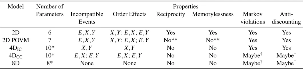
Not all models in our framework can cover all of the effects mentioned above. While the 2D model can cover all phenomena, the 2D POVM and 4D models can only predict order effects, violations of the Markov condition, and anti-discounting. The 2D POVM and 4D models cannot predict reciprocity and memoryless effects (except whenεis very small in the 2D POVM model).

The 8D model cannot cover any of these phenomena, except violations of the Markov condition and anti-discounting under specific configurations of the initial state. We note that it is possible for Bayesian models to produce order effects. In our modeling framework, the 8D model can be considered an ‘exchangeable’ Bayesian model. That is, the joint probability of any set of variables is independent of the ordering of those variables. However, more complex Bayesian models can violate the exchangeability property and produce order effects. For example, consider a Bayesian model with two additional variablesO1thatXis presented beforeY andO2thatY is

specifyingp(E)×p(Oi|E)×p(X|E,Oi)×p(Y|E,Oi,X), this approach simply redescribes the

empirical results. Also note that the causal power model is a special case of the more general 8D model and can at best cover the same phenomena as this model.

Table 1 summarizes the five models in our framework and the phenomena that each model covers. Our claim that different models correspond to particular styles of thinking in inference is an idea that has a precedence in literature. For example, Rehder’s (2014) theory of causal inference includes both normative and associative components. Our approach is similar, but our aim is to express all relevant influences (both normative and non-normative) within the same integrated, probabilistic framework.

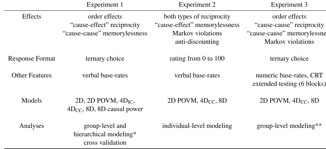
Table 2 provides a summary of the three experiments. Because there are a large number of different probability questions that can be asked when working with three binary variables (especially when you consider all of the different possible ways to condition on the variables), we took the approach of testing different questions in different experiments. The first row of Table 2 lists the effects tested in each experiment. In Experiment 1, we examine six different models (2D, 2D POVM, 4DIC, 4DCC, 8D, and 8D causal power). The modeling results of Experiment 1 show

that the 2D POVM and 4DCCmodels outperform the other two quantum models. Thus, we drop

the 2D and 4DICmodels from the analyses of Experiments 2 and 3. We also find that both the

general 8D model and 8D causal power models perform about the same. Thus, we drop the more restricted 8D causal power model from the analyses of Experiments 2 and 3. The table also provides an overview of the types of analyses that we perform for each experiment.

Experiment 1

The first experiment examines predictions of our modeling framework that have previously received less attention in the causal inference literature: order effects, reciprocity, and

categories. We selected this paradigm because we wanted participants to reason using linguistic descriptions of events rather than using statistical information or learning contingencies through observation. There seems little doubt that at least in some cases causal knowledge is acquired in such a direct, linguistic way, as opposed to using statistical information or learning contingencies through observation. Additionally, there is evidence that people’s judgments about causal systems often deviate from classical probability theory when tasks are presented using linguistic

descriptions (Sloman & Fernbach, 2011; Trueblood & Busemeyer, 2012; Rehder, 2014). Thus, we focus our efforts in this domain. In our task, participants are given a linguistic description of a novel category (e.g., African Lake Shrimp) and asked to judge the likelihood that certain features cause others. Specifically, participants are given information about how two independent features can influence a third feature. The language used to describe the features and their relationships is purposely vague as many real life situations do not involve precise information. Note that while our experiments use a paradigm similar to Rehder and Hastie (2001) and Rehder (2003b, 2003a), those previous studies did not examine the three effects of interest (order effects, reciprocity, and memorylessness). Thus, the aim of this experiment is part replication, and part examining these new effects. The data and models for all three experiments are available on the Open Science Framework at https://osf.io/4chu6/.

Methods

features (X,Y, andE) where two of the features (XandY) causally influenced the third (E), forming a common effect network. For example, in the African Lake Shrimp category,X₁= high amount of ACh neurotransmitter (X2= low amount of ACh),Y1= accelerated sleep cycle (Y2=

normal sleep cycle), andE1= high body weight (E2= low body weight ). Participants were given

information about the typicality of feature values. For example, they were told that “Most shrimp have a high amount of ACh whereas a few have a low amount of ACh”. In both categories, most animals had featureX1, a few had featureX2, a few had featureY1, and most had featureY2. Also,

half of the animals had featureE1and half had featureE2. Participants were also given the causal

relationships between features. These relationships were described as one feature causing another. In both categories,X1andY1were described as causingE1. Likewise, bothX2andY2were

described as causingE₂. Participants were also told that there were no known relationships betweenXandY. Details of the stimuli are given in Appendix B.

Participants first studied the three features and the typicality of their values. After studying this information, they took a multiple-choice test with six questions that tested them on this knowledge. Participants were required to answer each question correctly before moving on to the next one. Next, they studied the two causal relationships and took another multiple-choice test with eight questions testing them on this new knowledge. As before, participants were required to answer each question correctly before moving on to the next one. Finally, participants were asked to take a few minutes to review the features and relationships one more time. After they finished reviewing this information, they completed a third multiple-choice test with 10 questions. In this final test, participants were only given one opportunity to answer each question. Their score on this test was used to gauge how well they learned the features and causal relationships.

participants were told that a biologist caught a new animal (either shrimp or ant) in a particular location (e.g., Lake Victoria) and were queried about one of the features of that animal. For example, in the African Lake Shrimp category, they might be asked ”What type of body weight do you think this shrimp has?” (questionEin the table). Participants were given three response options: feature value 1, feature value 2, or equally likely to be feature value 1 or 2. For example, in the question about body weight, the response options were 1) a low body weight, 2) a high body weight, and 3) equally likely to be low or high.

Some of the questions required participants to make a sequence of decisions about a feature value (e.g.,E) as they learned new information about the other features (e.g.,XandY). For example, they might be asked about the body weight of a shrimp given lab tests that showed the shrimp had a high amount of ACh neurotransmitter (i.e.,E|X₁). Participants might then be asked to reevaluate body weight based on additional lab tests that showed the shrimp also had a normal sleep cycle (e.g.,E|X₁,Y2). Note that information about the value of the first feature (e.g.,X1)

remained on the computer screen when new information about the second feature (e.g.,Y2) was

presented. Thus, participants had access to all feature information during their final choice, which makes it less likely (if not impossible) that any observed effects result from memory failures.

Behavioral Results

We use Bayesian statistics for all analyses in this paper. All tests were implemented using the open source software package JASP (JASP Team, 2016). For each test, we report the Bayes factor (BF), which is a ratio quantifying the evidence in the data favoring one hypothesis relative to another. In particular, we report BF10, which is the evidence for the alternative hypothesis relative

to the null hypotheses. When BF10<1, there is evidence for the null hypothesis. When BF10>1,

there is evidence for the alternative hypothesis. The larger BF10, the more evidence there is in

favor of the alternative hypothesis. While Bayes factors are directly interpretable, labels for the strength of the Bayes factor have been proposed. In particular, BF greater (less) than 1, 3 (1/3), 10 (1/10), 30 (1/30) and 100 (1/100) are considered ‘Anecdotal’, ‘Moderate’, ‘Strong’, ‘Very Strong’ and ‘Extreme’ evidence respectively (Kass & Raftery, 1995). We also note the coarseness of the response scale (only three response options). For the analyses and modeling below, we only consider group level results. Experiment 2 uses a different response scale and allows for individual level analyses.

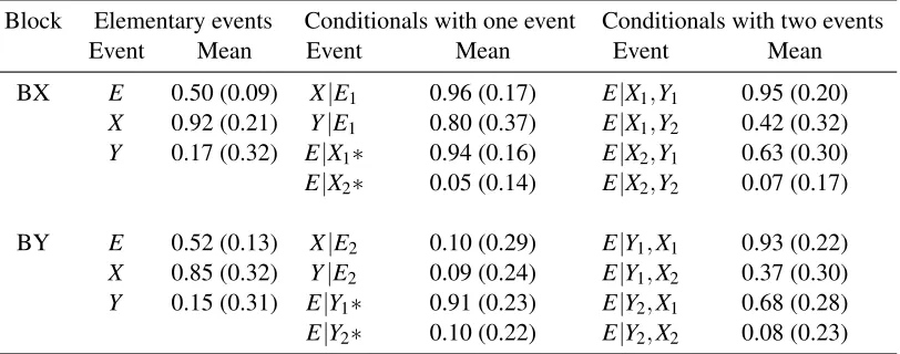
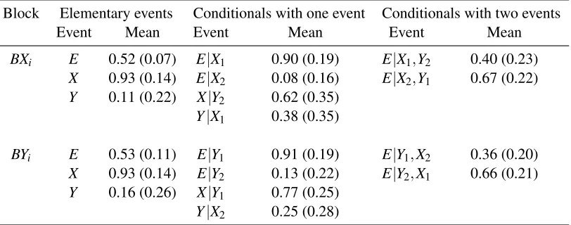
All participants were included in the analyses. The average score on the 10 question multiple choice test was 9.41 indicating most participants correctly learned the feature values and causal relationships during the first part of the experiment. For analyses of the choice data, we calculated achoice scorefor each participant in a similar way to Rehder (2014) by assigning the following values to the three response options: feature value 1 = 1, feature value 2 = 0, and equally likely = 0.52. Note that there were no differences between choices in the two different animal categories (BF10= 0.105) and so responses were collapsed for the following analyses. The mean

choice scores along with standard deviations for each question are given in Table 3.

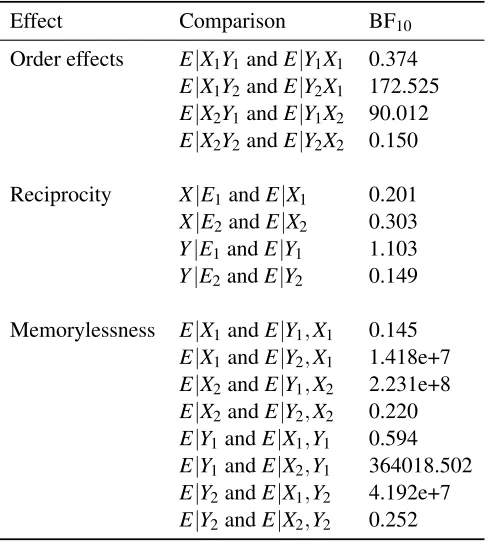
Order effects were assessed by comparing pairs of questions such asE|X₁,Y2andE|Y2,X1.

feature values matched (i.e., both X and Y equal to 1 or both equal to 2), showed no evidence for order effects. The lack of order effects for these questions could simply be due to floor and ceiling effects. As seen in Table 3, the mean choice scores for conditionals with two matching causes are either very close to 1 (when both X and Y equal 1) or very close to 0 (when both X and Y equal 2). On the other hand, there was ‘very strong’ to ‘extreme evidence’ for order effects when the feature values are mismatched. These order effects are easily seen in the mean choice scores reported in Table 3. The mean choice score forE|X1,Y2was 0.42 as compared to 0.68 forE|Y2,X1. Likewise,

the mean choice score forE|X₂,Y1was 0.63 as compared to 0.37 forE|Y1,X2. These results show

that participants place more weight on recent information, demonstrating a recency effect. Reciprocity or the inverse fallacy (Koehler, 1996; Villejoubert & Mandel, 2002) was examined by comparing pairs of questions such asX|E₁andE|X₁. As a reminder, there are two distinct ways to test for reciprocity. One way is to examine reciprocity between the effect and causes, called “cause-effect” reciprocity (e.g.,X|E₁versusE|X₁). The other way is to examine reciprocity between the two causes, called “cause-cause” reciprocity (e.g.,X|Y1versusY|X1). In

this experiment, we only examined “cause-effect” reciprocity. In Experiments 2 and 3, we examine “cause-cause” reciprocity.

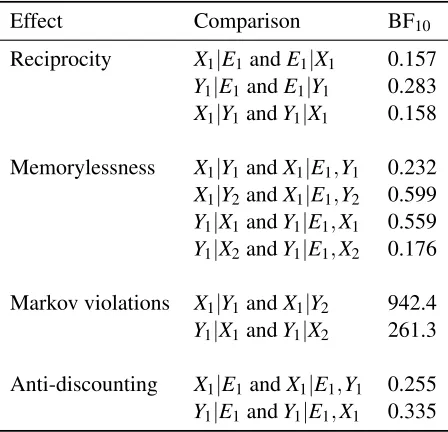
There are four possible comparisons that can be made by pairing the questions from both blocks. Bayesian paired samples t-tests were conducted on the four pairs and the results are reported in the middle of Table 4. Reciprocity occurs when the probability of one feature given another is the same as the probability when the features are reversed, e.g. p(E1|X1) =p(X1|E1). In

other words, reciprocity is an invariance and evidence for the effect is seen as evidence for the null hypothesis. Thus, when BF10<1, there is evidence for reciprocity. It is perhaps easier to evaluate

the strength of evidence for reciprocity if we rewrite the Bayes Factor so that evidence for the null hypothesis is in the numerator (i.e., BF01). This shows the effect ranges from BF01= 0.91

(‘anecdotal’ evidence for the alternative hypothesis) in the comparison ofY|E₁andE|Y₁to BF01=

Memorylessness occurs when the probability of a feature only depends on the most recent information given, e.g. p(E₁|X₁) =p(E₁|Y₁,X₁)sinceX₁is the most recent given information. Similar to reciprocity, there are different ways to examine memorylessness. One way is to examine the probability of the effect conditioned on the causes, called “cause-cause” memorylessness (e.g.,

E1|X1versusE1|Y1,X1). Another way is to examine the probability of a cause conditioned on the

effect and other cause, called “cause-effect” memorylessness (e.g.,X1|E1versusX1|E1,Y1). This

experiment examines “cause-cause” memorylessness. Experiment 2 examines “cause-effect” memorylessness.

There are eight possible comparisons that can test for this property. Bayesian paired samples t-tests were conducted on all eight pairs and the results are reported at the bottom of Table 4. Similar to reciprocity, memorylessness is an invariance and evidence for the effect is seen as evidence for the null hypothesis (i.e., when BF10<1). The evidence for memorylessness is mixed.

When the feature values of the causes match (i.e., both X and Y equal to 1 or both equal to 2), there is evidence for memorylessness. However, when the feature values of the causes are mismatched, there is strong evidence against memorylessness. In the case where feature values match, the result could simply be due to floor and ceiling effects because the mean choice scores in these questions are either very close to 1 or 0 (see Table 3).

Modeling Results

The behavioral results of Experiment 1 show evidence for order effects, reciprocity, and memorylessness (although evidence for the latter two effects is mixed). This recommends our modeling approach, which encompasses representations that can account for these effects. In this section, we explore this further by comparing six different models, ranging from fully quantum (all events are incompatible) to fully classical (no incompatible events).

Three Markov chain Monte Carlo (MCMC) chains were used with 50,000 samples and a burn-in of 5000 samples. Chain convergence was assessed using the ˆRstatistic, and all chains had good convergence behavior.

Unless otherwise noted, the priors for all angle variables were taken to be π

2×Beta(2,2). For

the general 8D model and two 4D models the priors for theρiivariables were taken to be uniform

in the interval[0,1]and then normalized to ensure∑iρii=1. For the causal power

parameterization of the 8D model, the priors forwX,wY,wa,p(X1)andp(Y1)were uniform in the

interval[0,1]. For the 2D and 2D POVM models it is more useful to set the priors to be

asymmetric, as this helps convergence. The reason for this is that the quantum models are invariant under certain transformations of the variables; restricting the range of theρvariable helps to avoid

different chains converging on apparently different parameter sets which are in fact equivalent. The 2D model is particularly prone to this, and so we set the prior forρto be uniform in the range

[.5,1]. The 2D POVM is less sensitive in this regard, and a prior forρtaken to be uniform in the

interval[.2,1]produced good convergence behavior. For the 2D POVM model the prior forεwas

taken to be uniform in the interval[0, .05], which is based on empirical fits in previous work (Yearsley & Pothos, 2016).

For model comparisons, we used JAGS to compute the deviance information criterion (DIC; Spiegelhalter, Best, Carlin, & Van Der Linde, 2002). The DIC is a generalization of the BIC, with smaller values indicating a better fit. The DIC includes a component related to the goodness of fit as well as a component related to model complexity (technically, the effective number of

parameters). Thus the DIC balances accuracy with parsimony. Note that the DIC is not directly interpretable, however differences between DIC values for models fit to the same data set can be interpreted. A difference in the DIC of 10 or more is usually taken to indicate a strong advantage in fit.

questions. We fit the models to these 19 questions. Because our models output probabilities rather than choices, we transformed each predicted probability by a softmax function (similar to Rehder, 2014) to simulate the fact that each participant is forced to choose between the three alternatives rather than outputting a probability judgment. Specifically, we assumed that individuals represent probabilities as log odds and that selecting optionxfollows the softmax rule:

choice(x) = exp( logit(px)

τ )

exp(logit(px)

τ ) +exp(

logit(1−px)

τ )

. (26)

wherepx is the predicted probability from the model andτis a “temperature” parameter that

controls the extremity of the responses. We then assumed that mean choice scores followed a beta distribution using the outputs of the softmax:

choice score∼Beta(λ×choice(x),λ(1−choice(x))) (27)

where the parameterλcontrols the variance. The prior forτwas taken to beN(0.1,0.01)and the prior forλwas uniform in the range[2,100]. Note that the addition ofλandτadds two parameters

to the parameter counts given in Table 1.

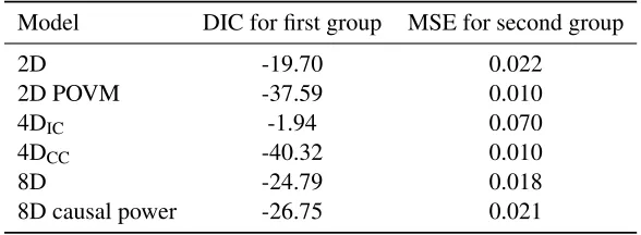
The DIC values for all six models are the following: 2D = -25.20, 2D POVM = -38.95, 4DIC

= -4.03, 4DCC= -42.55, general 8D= -25.32, causal power 8D = -25.88. The 4DCCand 2D POVM