Model selection, estimation and forecasting in INAR(p) models: A likelihood-based Markov Chain approach

Model Selection, Estimation and Forecasting

in INAR(p) Models: A Likelihood Based

Markov Chain Approach

Ruijun Bu

University of Liverpool, UK

Brendan McCabe

University of Liverpool, UK

December 4, 2007

Model Selection, Estimation and Forecasting

in INAR(p) Models: A Likelihood Based

Markov Chain Approach

Abstract

This paper considers model selection, estimation and forecasting for a class of integer autoregressive models suitable for use when analysing time series count data. Any number of lags may be entertained and estimation may be performed by likelihood methods. Model selection is enhanced by the use of new residual processes that are de…ned for each of the p+ 1 unobserved components of the model. Forecasts are produced by treating the model as a Markov Chain and estimation error is accounted for by providing con…dence intervals for the prob-abilities of each member of the support of the count data variable. Con…dence intervals are also available for more complicated event forecasts such as functions of the cumulative distribution function e.g. for probabilities that the future count will exceed a given threshold. A data set of Australian counts on medical injuries is analysed in detail.

1. Introduction

One of the objectives of modelling time series data is to forecast future values of the variables of interest. The most common procedure for constructing forecasts in time series models is to use conditional expectations as this technique will yield forecasts with minimum mean squared forecast error. However, this method will invariably produce non-integer-valued forecasts, which are thus deemed to lack data coherency in the context of count data models. This paper presents a method of coherent forecasting for count data time series based on the integer autoregressive, IN AR(p), class of models. Integer autoregressive models were introduced by Al-Osh and Alzaid (1987) and McKenzie (1988) for models with 1 lag. Both Alzaid and Al-Osh (1990) and Du and Li (1991) considered the

IN AR(p) class but with di¤ering speci…cations of the thinning operators. In this paper we use the conditionally independent thinning scheme of Du and Li (1991). Freeland and McCabe (2004b) suggest using theh-step ahead conditional distribution and its median to generate data coherent predictions in theIN AR(1) case. They also suggest that the probabilities associated with each point mass be modi…ed to re‡ect the variation in parameter estimation. McCabe and Martin (2005) explored the issue of coherent forecasting with count data models under the Bayesian framework but they too are only concerned with …rst-order case. More recently, Jung and Tremayne (2006) proposed a simulation based method for producing coherent forecasts for higher-order IN ARmodels but this too requires considerable computational work and does not use likelihood methods.

The paper makes three contributions. First, we suggest that the model be esti-mated by Maximum Likelihood (ML) should distributional assumptions warrant it1_{. We may therefore take advantage of the well known asymptotic normality} and e¢ ciency properties of the ML method. ML is not di¢ cult computationally and allows for a richer set of tools for model selection and improvement than do other methods of estimation for this class of models. For example, consider testing whether a thinning component should be excluded from the model i.e. testing if the associated parameter k = 0. Since k is a probability, methods of

estima-tion require that ^k be restricted to [0;1) and so tests based on ^k will have a

non-standard distribution because of the truncation at the boundary point0. This truncation is not an issue for score based tests in the ML framework. Other

tech-1_{Of course theIN ARmodel with Poisson arrivals could be used as a pseudo-likelihood with}

niques like multiple residual analysis and speci…cation testing are also available in the ML framework. Moreover, not only is the model estimated by ML but so too is the entire h-step ahead probability mass function. This provides an optimality property for this method of forecasting. Estimation uncertainty can be accom-modated by computing con…dence intervals for these probabilities. Secondly, we suggest that the forecast mass function be computed by using a Markov Chain (MC) representation of the model. The method, while simple, avoids the need to evaluate complicated convolutions and the same technique may be applied to any arrivals distribution and thinning mechanism. Thirdly, we consider forecasting the cumulative distribution function and events based on it. While it is undoubtedly interesting to know what the probability distribution of the size of a queue is, it is often more important to know what the probability that the number will exceed a certain critical threshold is. This requires forecasts of the cumulative distribu-tion funcdistribu-tion and con…dence intervals for the associated probabilities. The paper explains how con…dence intervals with the correct coverage may be constructed.

A data set consisting of counts of deaths (by medical injury), monthly from January 1997 to December 2003, is analysed by ML techniques. Lag selection is achieved by means of residuals analysis and speci…cation tests. The selected model is used to forecast up to8months ahead. Forecasts are made for both the probability mass and cumulative distribution functions.

The remainder of the paper is organized as follows. Section 2 outlines the

IN AR(p) model and brie‡y discusses its properties. In Section 3, we present a method for producing h-step ahead forecasts of the conditional probability dis-tribution of theIN AR(p) process. We also show how parameter uncertainty can be re‡ected in con…dence intervals for probability forecasts. The medical injury death count data is analysed in Section 4 while Section 5 concludes.

2. The INAR(p) Model

Du and Li (1991) de…ne theIN AR(p) model to be

Xt= 1 Xt 1+ 2 Xt 2+ + p Xt p+"t; (1)

where the innovation process _f"tg is i.i.d( "; 2") and is assumed to be

indepen-dent of all thinning operations k Xt k for k = 1;2; : : : ; p, which are in turn

onXt k, is de…ned as

k Xt k = X_Xt k

i=1 Bi;k;

where each collection_fBi;k; i= 1;2; :::; Xt kgconsists of independently distributed

Bernoulli random variables with parameter k and the collections are mutually

independent fork= 1;2; : : : ; p. Intuitively, k Xt k is the number of individuals

that would independently survive a Binomial experiment in a given period, where each of theXt kindividuals has identical surviving probability k. The case where

p = 1 and _f"tg is Poisson is known as Poisson autoregression, often denoted as

P oIN AR, since in this case the marginal distribution of Xtis also Poisson. When

p >1, it can be shown that the unconditional mean of Xt and the unconditional

variance of Xt are generally not equal, so that the marginal distribution of Xt is

no longer Poisson even though the innovations are. Dion et al. (1995) show that theIN AR(p) process may be generally viewed as a special multitype branching process with immigration. When k 2[0;1), the IN AR(p) process is

asymptot-ically stationary as long as Pp_k=1 k < 1 and the correlation properties of this

process are identical to the linear Gaussian AR(p) process according to Du and Li (1991).

The conditional moments ofXt are given by

E[XtjXt 1; : : : ; Xt p] = "+ p

X

k=1

kXt k

V ar[XtjXt 1; : : : ; Xt p] = 2"+ p

X

k=1

k(1 k)Xt k

and so while Xt is (unconditionally) stationary it is conditionally heteroscedastic

and so the process will exhibit volatility clustering. In contrast to an ARCH model, Xt is serially dependent and the heteroscedastic e¤ect disappears whenXt

is uncorrelated. In Bu et al. (2006), a representation of the conditional probability

P(XtjXt 1; : : : ; Xt p) is given for the IN AR(p) model with Poisson innovations

(IN AR(p)-P) as

P(XtjXt 1; : : : ; Xt p)

=

min(X_Xt 1;Xt)

i1=0

Xt 1

i1

i1

1 (1 1)Xt 1 i1

min(Xt_X2;Xt i1)

i2=0

Xt 2

i2

i2

min[Xt p;Xt_X(i1+ +ip 1)]

ip=0

Xt p

ip ip

p(1 p)Xt p ip

e Xt (i1+ +ip)

[Xt (i1 + +ip)]!

: (2)

By multiplying these conditional probabilities we may calculate the likelihood of the data conditional on the initialp observations. By means of the likelihood the parameters may be estimated. Other diagnostics including residuals may also be computed.

A natural way to de…ne residuals in theIN AR(p)-P model is to de…ne a resid-ual process for each component. So, generalising Freeland and McCabe (2004a), let k Xt k kXt k,t=p+ 1; :::; T, be the set of residuals for the kth thinning

process and let"t be residual set for the arrivals component. These de…nitions

as they stand are not practical, because k Xt k and "t are not observable but

we can replace k Xt k and "t respectively with Et[ k Xt k] and Et["t] (their

conditional expectations given the observed values of Xt; Xt 1; :::; Xt p). Thus,

we de…ne the computable residuals as

rkt =Et[ k Xt k] kXt k

and

r0t=Et["t] :

It is easy to see that adding the new sets of residuals gives the usual de…nition of residuals i.e.

p

X

k=0

rkt=Xt p

X

k=1

kXt k :

Thus, the usual residuals have been decomposed into sets that re‡ect each compo-nent of the model. However, it should be borne in mind that the decomposition is not orthogonal and the residual sets are correlated. The new residuals may easily be calculated, once the model is estimated, as Et[ k Xt k] andEt["t]are readily

available in terms of the conditional probabilities given in (2) i.e.

Et[ k Xt k] =

kXt kP(Xt 1jXt 1; : : : ; Xt k 1; : : : ; Xt p)

P(XtjXt 1; : : : ; Xt p)

;

Et["t] =

P(Xt 1jXt 1; : : : ; Xt p)

P(XtjXt 1; : : : ; Xt p)

:

3. Forecasting Conditional Distribution with the

IN AR

(

p

)

-P

Model

Coherent forecasting requires the conditional forecast distribution of the count variable at future periods. In the relatively simple case of P oIN AR model, the forecast distributions are convolutions of Poisson and Binomial random variables and an explicit expression for P (XT+hjXT) is given in Freeland and McCabe

(2004b). However, for the higher-order models of principal concern here, analytic solutions are not easily derived. In what follows, we present an e¢ cient procedure for producingh-step ahead distribution forecasts for theIN AR(p)-P model using the transition probability function of the process.

3.1. Forecasting the Conditional Probability Distribution: A Markov Chain Approach

We may think of any IN AR(p) process generated by (1) as a Markov process (chain) X which takes values at time t, Xt. In principle, the number of possible

states of the chain, being the values taken by the process, is in…nite. But given a data set, there typically exists a su¢ ciently large positive integerM such that the probability of observing a count larger than M is negligible. Therefore, for a given count seriesXt, we can assume that Xt takes values in the …nite collection

f0;1; : : : ; M_g. For example, consider the case wherep= 2. We think of the states of the system as given by pairs of consecutive values of the process. So at time

t 1, the chain could be in any of the states

S=_f(0;0);(0;1); :::;(0; M);(1;0);(1;1); :::;(0; M);(2;0)::::_g

as (Xt 2; Xt 1) takes values (i2; i1) 2 S. At time t the process moves to a new pair of values in the same state space and the transition probabilities of going from one state to another are given by

P(Xt=j1; Xt 1 =j2jXt 1 =i1; Xt 2 =i2) = P(Xt=j1jXt 1 =i1; Xt 2 =i2)

whenj2 =i1 and zero otherwise. The probability on the right is given by (2) with

p= 2 for the IN AR(p)-P model. The zero probability arises when j2 6=i1 since both values refer to the process X at the same time period t 1. This scheme may be extended to cater for larger values ofp. Hence, at any given periodtthere are(M + 1)p di¤erent states in the setS, determined by_fXt p+1; Xt p+2; : : : ; Xtg.

refers toXt p+1while the second refers toXt p+2and so on. Denote the(M+1)p 1vector,S(Xt), to be the elements of the vectors in the state setS that correspond

to Xt. For a Markov system with …nite states, the forecast distribution of each

state at any time t can be obtained by means of the transition matrix method. Let Q denote the (M + 1)p (M + 1)p transition probability matrix of an

IN AR(p)model with maximum possible countM. To get probability forecasts for each state, we let the(M+1)p 1probability vector, trepresent the probabilities

of …nding the system in each of the di¤erent states at a given periodt. Also de…ne, for each i _{2 f}0;1; :::; M_g, a (M + 1)p _{1 selection vector s}

i, which has M + 1

entries equal to 1 in positions that correspond to those in S(Xt) where Xt = i;

all other entries in si are zero. Thus, the probability of Xt =i can be written as

0

tsi. Hence, for a general IN AR(p) process the conditional probability forecasts

for XT+h can be obtained from the forecasts of the probability vector T+h. That

is

P (XT+h =ijXT; : : : ; XT p+1) = 0T+hsi:

The following results are well known from the theory of Markov chains (see for example Kemeny and Snell (1976)). LetQ andQ(h) _{denote, respectively, the} one-step transition matrix and h-step transition matrix for a homogeneous pth-order Markov system. Then

Q(h) =Q(h 1)Q=Qh; (3)

and

0

T+h = 0T+h 1Q= 0TQ

h_{: (4)}

Equation (3) says that the h-step transition matrix is equal to the hth power of the one-step transition matrix and Equation (4) says that the h-step ahead forecast of the probability vector T+h is equal to the current probability vector

T times the h-step transition matrix. Thus the current probability vector and

the1-step ahead transition matrix are all that is required to produce forecasts for any number of periods ahead. We may summarise the foregoing developments in the following proposition.

Proposition 3.1. For a generalIN AR(p)process with maximum possible count

assumed to be M, the h-step ahead forecast of the conditional probability of

XT+hjT =i; i= 0;1; :::; M is given by

P (XT+h =ijXT; : : : ; XT p+1) = 0TQ h_s

i; (5)

where 0

T is probability of the current state of the system, si is a selector vector

the process. The transition matrix for theIN AR(p)-P process may be calculated

from (2) which depends on the underlying parameters 1; :::; p and .

A method for assessing the uncertainty associated with probability forecasts (5) due to parameter estimation is presented in the next section.

3.2. Forecasting the Conditional Distribution When Parameters are Es-timated

If the parameters of the model were known it would be easy to calculate the conditional probability forecastsP (XT+h =ijXT; : : : ; XT p+1) directly using the results of Proposition 3.1. However, in almost all practical applications these parameters are unknown and have to be estimated. Therefore, it is important that this source of variation be accounted for when producing forecasts. In the current context, the values taken by the process in the future are not in doubt; they are low counts and are the elements of_f0;1; ::; M_g. The unknown quantities are the probabilities P(XT+h =ijXT; : : : ; XT p+1); i = 0;1; :::; M and it is these that must be estimated. We abbreviate these conditional probabilities (in the manner of conditional expectations) to PT (XT+h =i). Estimation uncertainty is

the error made in estimating these probabilities. This error is in turn a function of the error made in estimating the unknown parameters implicit inPT (XT+h =i)

with these probabilities speci…ed in Proposition 3.1 for theIN AR(p)-P model. Let = ( 1; :::; p; ) be the parameter vector of theIN AR(p)-P model. The

h-step ahead forecast of the conditional probability mass function is written as PT (XT+h =i; ) to underline dependence on the parameters. Under

stan-dard regularity conditions, the ML estimator of , denoted ^, is asymptoti-cally normally distributed around the true parameter value, i.e. pT(^ 0)

a

N(0;i 1) where i 1 is the inverse of the Fisher information matrix. Let gi(^) =

^

PT (XT+h =i) = PT XT+h =i;^ , i = 0; :::; M and de…ne a vector function

g(^) = g0(^); :::; gM(^)

0

estimated probabilities of more complex events. The following proposition is a straightforward consequence of Ser‡ing (1980, Section 3.3).

Proposition 3.2. For the IN AR(p)-P model, the ML estimator of the h-step ahead forecast,g(^), has an asymptotically normal distribution with mean vector

g( 0) and variance matrix

V( 0) =T 1Di 1D0; (6)

whereiis the Fisher information matrix and D= @g( )=@ 0_{j =}

0 is a(M + 1)

(p+ 1) matrix of partial derivatives.

Expressions for these derivatives are available in Bu et al (2006). The elements on the diagonal ofV( 0)are the variances of the estimated forecast probabilities for each possible value on its support and the o¤-diagonal elements represent the covariances between estimated forecast probabilities for di¤erent possible values. Accordingly, estimators of the forecast probabilities for di¤erent values of i will be correlated. By Proposition 3.2, marginal 95% con…dence intervals for the conditional probability P(XT+h = ijXT; : : : ; XT p+1; 0) for i = 0;1; : : : ; M, can be computed, using its asymptotic distribution, by means of

^

PT (XT+h =i) 2 i+1(^);

where 2i+1(^) is the (i+ 1; i+ 1) element of V(^). While we may compute ^

PT (XT+h =i) for every i = 0;1; : : : ; M to obtain pointwise probabilities of the

entire mass function, the correlation between P^T (XT+h =i) and P^T (XT+h =j)

makes interpretation very di¢ cult when more than a single value ofiis involved. This correlation may be extremely large i.e. very close to+1 and negative corre-lation is also possible. Thus, when one is interested in events like(XT+h i)the

cumulative distribution function should be used.

Many more complicated events may, in turn, be written as mappings of g; often a linear function c0_g(^_{) of g(}^_{) will su¢ ce. Another application of the}

delta method gives the asymptotic distribution of these mappings, e.g. c0_g(^_{) is}

distributed as

N c0g( 0);c0V( 0)c : (7)

For example, let c0_g(^_{) =`}0

ig(^) where`i is a vector with the …rsti+ 1 elements

…rst i+ 1 elements of g and gives cumulative probabilities i.e.

^

PT (XT+h i) = i

X

j=0 ^

PT(XT+h =j)

and, from (7), the appropriate variance for P^T(XT+h i) is the sum of all the

elements in the (i+ 1) (i+ 1) top left submatrix of V( 0), estimated by V(^). Thus we may forecast the cumulative distribution function and obtain valid con-…dence intervals.

Another example is the probability of high or low counts. Say we are interested in the estimated probability of the future event, (u > l)

(XT+h l) or (XT+h > u)

which may be calculated by adding P^T(XT+h l) to 1 P^(XT+h u). A valid

con…dence interval is given by

1 + ^PT(XT+h l) P^(XT+h u) 2

q

c0_V(^_)c

where c0 _{= (`}

u `l)0 with `i de…ned as above. In this manner, we may obtain

valid con…dence intervals for the probabilities of fairly arbitrary complex events based on the individual outcomes.

4. Analysis of Injury Data

4.1. The Data

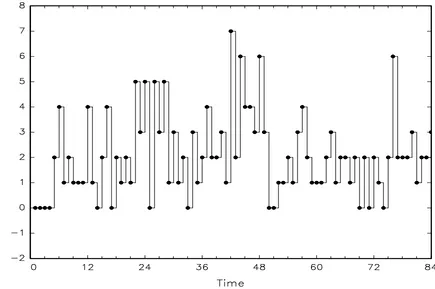
In this section, we apply the method developed to monthly counts of medical injury deaths in Australia. This data set, …rst analysed in Snyder et al (2007), consists of 84counts recorded from January 1997 to December2003. In the …rst instance we conduct some preliminary analysis to get an overall picture of the data at hand. Figure 1 provides the time series plot of the data, which shows neither discernible trends nor clear seasonal patterns. A summary of simple descriptive statistics for the data is given in Table 1. It can be seen that the observed counts vary from 0 to 7 with the sample mean and variance equal to 2:083 and 2:656, respectively. This suggests that there is some slight overdispersion in the data. The marginal distribution of these data is depicted in Figure 2.

4.2. Model Selection

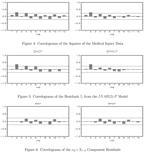
For forecasting purposes, we leave out the last 8 observations (10 percent of the whole sample) and use the …rst76 data points to select and estimate the model. Figures 3 and 4 plot the sample autocorrelation function (SACFs) and sample partial autocorrelation function (SPACFs) of the process as well as those of the squares. From Figure 3 we conclude that there is correlation in the levels of the process to be modelled though it is not exceptionally large. Interestingly, Figure 4, for the squares process, also reveals signi…cant correlation in the volatility a fact that is also apparent when one closely examines the time series plot in Figure 1.

[Figure 3] [Figure 4]

Figure 3 shows that the SACFs are signi…cant at both lag 2 and lag 4 at 5% signi…cance level. This is indicative of the presence of serial dependence in the series. However, no signi…cant seasonal patterns are found. Results of the Ljung-Box portmanteau test with various lag lengths (not reported) also con…rm the presence of serial dependence in the data. This and the existence of volatility clustering in Figure 4 indicates that the IN AR-P class is a reasonable set of models to consider. Meanwhile, the SPACFs is signi…cant at lag2, which suggests that an autoregressive model with dependence of order 2 may be a reasonable starting point.

Based on the above analysis, we decided to proceed by estimating anIN AR(2)

-P model. Estimation ofIN AR(p)-P models can be carried out in several di¤erent ways. These include the moments based Yule-Walker (YW) estimation method, the conditional least squares (CLS) estimation method of Klimko and Nelson (1978), and the maximum likelihood (ML) estimation of Bu et al. (2006). Bu (2006) provided detailed accounts of the three estimation methods and examined both the asymptotic e¢ ciency and …nite sample performance of the ML estimator (MLE) in relation to both the YW and CLS estimators. It is concluded that even in …nite samples it is worth the e¤ort to use MLE for gains in terms of both the bias and the mean squared error (MSE). For this reason, we decided to estimate the model by conditional (on the initial observations) ML (CML). Details of CML estimation ofIN AR(p)-P models are discussed in Bu et al. (2006)2_{. The}

2_{Bu (2006) also suggested a procedure for computing the unconditional likelihood but this}

CML estimates of the parameters are b1 = 0:058(0:094), b2 = 0:236(0:095), and

b= 1:537(0:291), respectively. The estimated asymptotic standard errors, which are obtained from the inverse of the observed Hessian, are given in the parenthesis adjacent to each estimate. As the model is estimated by maximum likelihood, it is straightforward to obtain the corresponding AIC and BIC values for the …tted model, which may be used as indications of overall suitability amongst alternative models. The AIC and BIC for the estimated IN AR(2)-P model are 273:39 and 280:38, respectively.

To assess the adequacy of the …tted model, we examine the residuals for serial dependence. The estimated Pearson residuals of the …tted IN AR(2)-P model are de…ned by_b"t=Xt b1Xt 1 b2Xt 2 b. In principle, the existence of any depen-dence structure in the residuals would suggest that a more general speci…cation is called for. For this reason, we plot the SACFs and SPACFs of b"t in Figure 5.

Informally, the …gure indicates that there is no obvious dependence structure left in the residuals. Results from the Ljung-Box portmanteau tests with various lag lengths (not reported) also do not allow us to reject this hypothesis. However, it should be noted that the residual series_b"tis an aggregate measure of the residuals

from each stochastic component of the model. The results obtained by examining b"t do not necessarily re‡ect the suitability of each individual component.

[Figure 5]

For this reason, we inspect the SACFs and SPACFs for all three residual processes from the estimatedIN AR(2)-P model. While the SACFs and SPACFs for both 1 Xt 1 residuals and arrivals residuals (not reported) are all non-signi…cant up to lag 20 at all conventional signi…cance levels, the SACFs and SPACFs for the 2 Xt 2 residuals, given in Figure 6, are both signi…cant at lag 4, with the p-values being 0:044 and 0:065, respectively. The presence of serial dependence in 2 Xt 2 residuals is also supported by the portmanteau test which yields a test statistic ofQ(4) = 8:170 (p-value=0:017). These …ndings suggest that examining only the traditional residuals is not su¢ cient on its own and that the component residuals are useful tools for detecting the suitability of each component in the model. When combined with the analysis of the usual residuals, they provide a more thorough and robust investigation into the goodness of …t of the estimated model.

The results above suggest that a more generalIN AR(4)-P model with Poisson arrivals be investigated. We expect that by doing this we should be able to eliminate the 4th order dependence in the residuals. As before, the model is estimated using conditional maximum likelihood. It is important to note that the thinning parameters are de…ned in the range[0;1). This requires restrictions to be imposed on each parameter during estimation. The constrained CML estimation results inb3 = 0. We therefore proceed to estimate anIN AR(4)-P model without the 3 Xt 3component. The CML estimates of the parameters and the associated standard errors are found to be _b1 = 0:015(0:095), b2 = 0:158(0:105), b4 = 0:137(0:103), andb= 1:550(0:332), respectively. From an inspection of the SACFs and SPACFs for both the Pearson residuals and all four component residuals (three thinning processes and one arrival process), we conclude that these residuals correspond to white noise processes and therefore that an IN AR(4)-P model without 3 Xt 3 is adequate in explaining the serial dependence in the data. Meanwhile, the AIC and BIC values for the estimated model reduce to 267:10 and 276:43, respectively, which is also indication of the improved speci…cation.

For forecasting purposes, we tend to prefer a model that is parsimonious to avoid in-sample over …tting. We note from the …tted IN AR(4)-P model that b1 is fairly small relative to its standard error, suggesting that the …rst thinning operation process may not be statistically signi…cant. However, a formal test is needed to con…rm this hypothesis. Unlike GaussianAR(p)models, the hypothesis

1 = 0forIN AR(p)models is on the boundary of the parameter space. Therefore, we cannot simply apply the usual test based on the ratio of the parameter estimate to its standard error. Nevertheless, since the model is estimated by ML, the boundary problem in the testing of coe¢ cient signi…cance may be avoided by using a Lagrange Multiplier (LM) test. Unlike the Wald test and the likelihood ratio test, the LM test is valid even when the null hypothesis corresponds to a boundary value of the parameter space. To perform the desired test, we thus estimate the above model by imposing the restriction that 1 = 0and calculate the LM statistic based on the restricted estimates. The LM statistic is given by `_0

bRi

1

bR

_

`_b

R where

_

`0_b

R andibR are the score vector and information matrix for the unrestricted model

evaluated at the restricted estimatebR. Explicit expressions for the score function

dropping the 1 Xt 1 component and use the restricted model (the IN AR(4)-P model with only 2 Xt 2 and 4 Xt 4 as thinning components) for further analysis. The conditional maximum likelihood estimates for the restricted model are b2 = 0:158(0:104), b4 = 0:138(0:103), and b= 1:578(0:276), respectively. For the restricted model, neither the SACFs and SPACFs nor the portmanteau Q-tests would allow us to reject hypothesis that Pearson residuals and component residuals are white noise processes. In addition, the AIC and BIC values reduce further to 265:12and272:12respectively, suggesting improvement. The Information Matrix test of the overall adequacy of the model, given in Freeland and McCabe (2004a), has p-value 0:335 and so does not reject the reduced speci…cation. This is the …nal reduction of the forecasting model.

A further LM test on the joint hypothesis that 2 = 4 = 0 gives LM = 5:127, which corresponds to ap-value of0:077 relative to the 2(2). This provides evidence against the use of the naive i.i.d. Poisson model. Moreover, the AIC and BIC for the naive i.i.d Poisson model are 284:64 and 286:97, respectively, which are well in excess of those for the chosen IN AR(4)-P model. Finally, we conducted simulation experiments (not reported) to con…rm that the performance of the MLE, in terms of bias and MSE, was satisfactory at T = 76 and the LM test had, approximately, the size suggested by the asymptotic approximations.

4.3. Forecasting the Medical Injury Data

This section applies the method developed in Section 3 to produce forecasts for the medical injury data based on the …tted model. For a model with maximum lag length equal to 4, the h-step ahead conditional probability depends on the last 4 observations and can be denoted as P(XT+hjXT; XT 1; XT 2; XT 3); for

simplicity, it is henceforth denoted by PT(XT+h). When the parameters of the

model are estimated we use the notation P^T(XT+h). It is observed that the last

four observations of the series areXT = 6, XT 1 = 2, XT 2 = 0, and XT 3 = 1, respectively, whereT = 76.

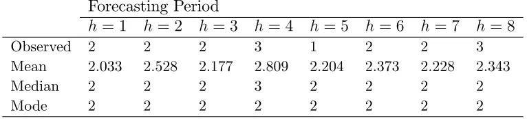
Table 2 gives the4-period ahead conditional mean, median and mode forecasts. As expected the conditional mean forecasts are no longer integer values. (In results unreported it can be seen that these conditional mean forecasts converge to the mean of the marginal distribution. This is equal to the unconditional mean of the process implied by the parameter estimates. Similarly, the conditional median and mode forecasts converge to their marginal counterparts.)

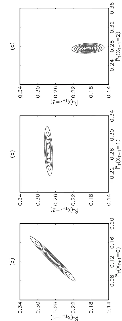
We apply the propositions proposed in Section 3 to compute point estimates and con…dence intervals for the probabilities associated with each value of the forecast distribution. These interval forecasts are given in the top panel of Table 3 in the form of the point estimate plus and minus two standard errors. Thus in theT + 1 period the point estimate of the probability of the value0 occurring is 0:126 and we are 95% con…dent that the probability lies between 0:126 0:049; However, it is not easy to interpret multiple rows from Table 3 simultaneously. Figure 7 gives three examples of the contours of the joint probability density functions of the estimated probability forecasts for pairs of possible counts. The probability forecasts are calculated by the delta method and so the joint probabil-ity densprobabil-ity functions of the probabilprobabil-ity forecasts for any pair of possible counts are asymptotically bivariate normal. It can be seen from these contours that the es-timated probability forecasts for di¤erent counts are correlated. For instance, the contour plot in Figure 7(a) suggests that the estimated conditional probabilities

^

PT (XT+1 = 0) andP^T (XT+1 = 1)have a near perfect positive correlation (0:980) while Figure 7(b) shows a weaker correlation (0:323) between P^T (XT+1 = 1) and

^

PT (XT+1 = 2). In contrast, Figure 7(c) suggests a negative correlation ( 0:157) between P^T(XT+1 = 2) and P^T(XT+1 = 3).

[Table 3] [Figure 7]

In many circumstances one is often more concerned with the conditional cumu-lative distribution forecasts and here too account must be taken of the correlation between individual forecasts. For example, in the current context, having mul-tiple deaths caused by medical injuries in any single month may be regarded as being very serious and thus the probability of having a count of more than 1, i.e.

PT (XT+h >1), may have particular signi…cance. Although cumulative

probabil-ities can be easily inferred from the top panel of Table 3 by summing over the corresponding point probability estimates, the appropriate standard errors can-not be directly inferred from the individual standard errors as the variance of a cumulative probability depends on o¤-diagonal elements ofV( 0)in (6) and these covariances are, as we have seen, rarely negligible.

between0:392 0:101. Equally, the estimate of the probability of having a count greater than1 is0:608 with a 95% con…dence interval equal to 0:608 0:101.

5. Conclusion

In this paper, we extend the ideas of Freeland and McCabe (2004b) and develop a method for producing data coherent forecasts for higher-order IN AR models. We show that the IN AR(p) process can be regarded as a Markov system and the forecasts of the distribution of a count series can be obtained by means of a transition matrix of the process. A procedure for calculating con…dence intervals for these forecast probabilities is also suggested.

An empirical analysis of Australian medical injury data under a Maximum Likelihood framework is conducted. Estimates of parameters of the IN AR(p)

-P model are obtained by conditional maximum likelihood estimation. Issues of model adequacy are also examined. Our analysis shows that the analysis of tra-ditional residuals alone may ignore serial dependence in the component residuals and that these latter are useful tools for detecting model misspeci…cation. We ap-ply the method developed to produce distribution forecasts for the medical injury data. The results show that the estimated point mass forecasts are more infor-mative than those supplied by either the mean, median or mode of the forecast distributions. In particular, we show that it is also possible to obtain forecasts of the cumulative probabilities as well as their associated con…dence intervals. Given the relatively small sample size on which the forecast experiments in this study are based, it is di¢ cult to perform robust statistical tests on the predictive accuracy of competing models as in, for example, Corradi and Swanson (2006). Never-theless, our analysis does indicate the potential bene…t of having constructive model selection tools available for analysing count data and improving forecast performance.

References

Al-Osh, M.A., & Alzaid, A.A. (1987). First-order integer valued autoregressive (INAR(1)) process.Journal of Time Series Analysis, 8, 261-275.

Bu, R. (2006). Essays in …nancial econometrics and time series analysis. Ph.D Thesis, University of Liverpool.

Bu, R., Hadri, K., & McCabe, B.P.M. (2006). Maximum likelihood estimation of higher-order integer-valued autoregressive processes. Working paper, University of Liver-pool.

Corradi, V., & Swanson, N.R. (2006). Predictive density and conditional con…dence interval accuracy tests. Journal of Econometrics, 135, 187-228.

Dion, J.P., Gauthier, G., & Latour, A. (1995). Branching processes with immigration and integer-valued time series.Serdica,21, 123-136.

Du, J.G., & Li, Y. (1991). The integer-valued autoregressive (INAR(p)) model.Journal of Time Series Analysis, 12, 129-142.

Freeland, R.K., & McCabe, B.P.M. (2004a). Analysis of low count time series by Poisson autoregression.Journal of Time Series Analysis, 25, 701-722.

Freeland, R.K., & McCabe, B.P.M. (2004b). Forecasting discrete valued low count time series.International Journal of Forecasting, 20, 427–434.

Jung, R.C., & Tremayne, A.R. (2006). Coherent forecasting in integer time series mod-els.International Journal of Forecasting, 22, 223-238.

Kemeny, J.G., & Snell, J.L. (1976). Finite Markov Chains. New York: Springer.

Klimko, L.A., & Nelson, P.I. (1978). On conditional least squares estimation for sto-chastic processes.Annals of Statistics, 6, 629-642.

McCabe, B.P.M., & Martin, G.M. (2005). Bayesian predictions of low count time series. International Journal of Forecasting, 21, 315-330.

McKenzie, E. (1988). Some ARMA models for dependent sequences of Poison counts. Advances in Applied Probability, 20, 822-835.

Ser‡ing, R.J. (1980). Approximation Theorems of Mathematical Statistics. New York: Wiley.

Table 1: Descriptive Statistics of the Medical Injury Data

Minimum Maximum Median Mode Mean Variance

0 7 2 2 2:083 2:656

Table 2: Mean, Median and Mode Forecasts and the Observed Values Forecasting Period

h = 1 h= 2 h= 3 h= 4 h= 5 h= 6 h= 7 h = 8

Observed 2 2 2 3 1 2 2 3

Mean 2.033 2.528 2.177 2.809 2.204 2.373 2.228 2.343

Median 2 2 2 3 2 2 2 2

Mode 2 2 2 2 2 2 2 2

Table 3: Forecasts for the Medical Injury Data ^

PT(XT+h =i)

h i= 0 i= 1 i= 2 i= 3

1 0.126 0.049 0.266 0.053 0.276 0.010 0.186 0.034 2 0.073 0.095 0.199 0.144 0.261 0.054 0.222 0.061 3 0.111 0.043 0.247 0.052 0.271 0.012 0.197 0.029 4 0.056 0.056 0.166 0.099 0.241 0.055 0.228 0.025 5 0.111 0.049 0.243 0.059 0.267 0.011 0.196 0.031 6 0.094 0.052 0.221 0.071 0.262 0.024 0.207 0.030 7 0.109 0.050 0.240 0.061 0.267 0.013 0.198 0.031 8 0.097 0.053 0.225 0.072 0.263 0.022 0.205 0.031

^

PT(XT+h i)

h i= 0 i= 1 i= 2 i= 3

Figure 1: Time Series Plot of the Medical Injury Data

Figure 3: Correlograms of the Medical Injury Data

Figure 4: Correlograms of the Squares of the Medical Injury Data

Figure 5: Correlograms of the Residuals_b"t from the IN AR(2)-P Model

F

ig

u

re

7

:

C

o

n

to

u

r

P

lo

ts

o

f

th

e

B

iv

a

ri

a

te

D

en

si

ti