White Rose Research Online
[email protected]
Universities of Leeds, Sheffield and York
http://eprints.whiterose.ac.uk/
This is an author produced version of a paper published in
Combustion Theory
and Modelling
.
White Rose Research Online URL for this paper:
http://eprints.whiterose.ac.uk/10273/
Published paper
Sharpe, G.J. (2008)
Effect of thermal expansion on the linear stability of planar
premixed flames for a simple chain-branching model: The high activation
energy asymptotic limit.
Combustion Theory and Modelling, 12 (4). pp. 717-738.
Combustion Theory and Modelling
Vol. 00, No. 00, February 2006, 1–19
Effect of thermal expansion on the linear stability of planar premixed flames for a simple chain-branching model: the high activation energy asymptotic limit.
G. J. Sharpe∗
School of Mechanical Engineering, University of Leeds, Leeds, LS2 9JT, UK
(Received 00 Month 200x; In final form 00 Month 200x)
The linear stability of freely propagating, adiabatic, planar premixed flames is investigated in the context of a simple chain-branching chemistry model consisting of a chain-branching reaction step and a completion reaction step. The role of chain-branching is governed by a crossover temperature. Hydrodynamic effects, induced by thermal expansion, are taken into account and the results compared and contrasted with those from a previous purely thermal-diffusive constant density linear stability study. It is shown that when thermal expansion is properly accounted for, a region of stable flames predicted by the constant density model disappears, and instead the flame is unstable to a long-wavelength cellular instability. For a pulsating mode, however, thermal expansion is shown to have only a weak effect on the critical fuel Lewis number required for instability. These effects of thermal expansion on the two-step chain-branching flame are shown to be qualitatively similar to those on the standard one-step reaction model. Indeed, as found by constant density studies, in the limit that the chain-branching crossover temperature tends to the adiabatic flame temperature, the two-step model can be described to leading order by the one-step model with a suitably defined effective activation energy.
1 Introduction
Freely propagating premixed flames may, in principal, exist as planar and steady waves. However, experi-ments show that in many cases the flame is actually wrinkled and time-dependent [1–4]. These ‘cellular’ or ‘pulsating’ flames may be regarded as the outcome of thermal-diffusive and/or hydrodynamic instabilities. Hence a first step in understanding their origins and onset is a linear stability analysis of the underlying steady, planar flame.
Much of the fundamental theory of combustion employs a standard, exothermic, one-step chemistry model [1, 4], F→P, where F denotes the fuel and P denotes the combustion products. This model predicts an adiabatic flame structure consisting of a diffusive pre-heat zone, followed by a thin reaction zone at the downstream end of the flame, where the fuel is consumed and all the heat is released. In the asymptotic limit of high activation energy, the reaction zone can be replaced to leading order by a reaction sheet or surface across which suitable jump conditions apply, and such that no chemical reaction or heat release occurs on either side of this reaction sheet. This asymptotic limit of the one-step model has been successfully employed in a number of linear stability studies of premixed flames. Sivashinsky [5] first employed a constant density approximation in order to study purely thermal-diffusive effects on the flame stability. The constant density model (CDM) used by Sivashinsky [5] ignores any hydrodynamic effects, and is formally valid only in the limit of small heat of reaction. Several workers then independently obtained long-wavelength asymptotic solutions of the linear stability problem, in the context of the Reactive Navier-Stokes equations [6–8]. These ‘slowly varying flame’ analyses capture mainly hydrodynamic effects on the flame stability. Jackson and Kapila [9] then solved numerically the one-step high-activation energy asymptotic linear stability problem for arbitrary perturbation wavelengths, and showed how the combination of both thermal-diffusive and hydrodynamic effects are important in determining the stability of premixed flames. These asymptotic one-step reaction studies also entail a near-equidiffusional flames (NEF) approximation, i.e they are valid for Lewis numbers asymptotically close to unity.
Finite activation energy numerical linear stability studies, which do not invoke the asymptotic limit, have also been performed for the one-step reaction model, both in terms of the CDM [10] and the Reactive Navier-Stokes equations [11, 12]. These studies show that, when the Lewis number is sufficiently far from unity, very high activation energies may be required for the asymptotic results to be quantitatively
predic-∗Corresponding author. E-mail: [email protected]
Combustion Theory and Modelling
ISSN 1364-7830 (print) / ISSN 1741-3559 (online) c2006 Taylor & Francis Ltd. http://www.tandf.co.uk/journals
tive. However, these finite activation energy studies do not reveal any qualitatively different instabilities than those predicted by the asymptotic analyses, even when the activation energy is quite moderate. The main use of such finite activation energy calculations is hence to provide quantitative test problems for numerical codes designed to simulate the fully non-linear flame evolutions [10, 13].
Although the one-step model has been very successful in describing and predicting many aspects of flame phenomena [1, 4], it fails to capture some aspects of hydrocarbon and hydrogen flame structures [4, 14]. In these flames, there any many intermediate steps between the conversion of fuel into products. These include chain-branching reactions, which produce a net increase in intermediates species such as radicals. The chain-branching reactions tend to have high-activation energy, and are hence active in the high-temperature regions of the flame, where they convert the fuel into intermediate species [14]. The intermediate molecules produced may then diffusive forwards and backwards over the entire flame structure, so that the ‘pre-heat’ zone is in reality also chemically active [4, 14]. Completion reactions, which remove the intermediates and convert them into products, tend to be temperature insensitive but highly exothermic, so that heat release occurs throughout the flame [4], in contrast to in a narrow region at the downstream end of the flame structure as predicted by the one-step model. Indeed, the exothermic completion reactions continue even after the fuel has been completely converted into intermediates, so that the fuel is exhausted interior to the flame, i.e. before the adiabatic flame temperature is reached at the downstream end [14].
This discrepancy between the one-step model and real flame structures motivates the need for a chemistry model which better mimics the effects of chain-branching outlined above. For the purposes of the mathe-matical theory of flames, however, any improved model should still be sufficiently simple and generic such that transparent, fundamental insights can be obtained and that some analytical or asymptotic progress is still possible. In this spirit, Dold and co-workers [14–16] have suggested a two-step chemistry model, consisting of a single chain-branching step, F+Y→2Y, and a single completion reaction step, Y+M→P+M, where Y represents a lumped or ‘pooled’ amalgam of intermediate species, and M is any species required to trigger the completion reactions, but is unchanged in the process. In the simplest version of this model, the branching reaction is assumed to have a high activation temperature but is thermally neutral, while the completion reaction is assumed to be temperature insensitive but releases all the heat. Dold [14] gives a very detailed discussion which puts the two-step model and its assumptions into the context of hy-drogen and hydrocarbon oxidation, including how the model parameters can be fitted to hyhy-drogen and hydrocarbon flame structures as predicted from detailed chemistry calculations.
Fundamental to the two-step model described above is the concept of a chain-branching crossover tem-perature,Tc, which, in regards to flame structure, is the temperature at which the rate of chain-branching
balances the rate of removal of intermediates by diffusion [14]. Thus above this temperature a chain-branching explosion occurs in which the fuel is converted rapidly into intermediates. For large activation energies of the branching step, the reaction is then active only in a narrow region occurring at temperatures close toTc. As for the one-step reaction, in the asymptotic limit of infinite activation energy, the branching
reaction can be replaced to leading order by a reaction sheet across which appropriate jump conditions apply. For the two-step model, the reaction sheet occurs at the crossover temperature, where the fuel is consumed.
As well as being able to mimic the main features of real flames which the one-step model can not, the two-step model also has mathematical advantageous over the one-step model. Firstly, the simple chain-branching model does not suffer from the well known ‘cold-boundary difficulty’ inherent in the one-step model [17]. Secondly, in the large activation energy asymptotic limit, the jump conditions across the reaction sheet are linear in the variables [14], as compared to the more complex jump conditions of the one-step model, which are non-linear in the temperature at which the reaction sheet occurs [1]. Further, in terms of the asymptotic flame stability, the two-step model does not require the NEF approximation and hence is valid for arbitrary values of the Lewis numbers [14].
Re-active Navier-Stokes equations. The main purpose of the paper is hence to compare and contrast with both the two-step CDM [14] and the one-step chemistry Reactive Navier-Stokes predictions [9]. Indeed, the paper should be viewed as the two-step analog of the one-step linear stability study of Jackson and Kapila [9].
2 The Model
The governing equations of the model are the quasi-isobaric Navier-Stokes equations coupled to the two-step chemistry scheme F+Y→2Y, Y+M→P+M. The non-dimensional versions of these equations are, in
two spatial dimensions, xand y,
∂ρ ∂t +
∂(ρu)
∂x + ∂(ρv)
∂y = 0, (1)
ρ∂u ∂t +ρu
∂u ∂x +ρv
∂u ∂y +
∂P ∂x =P r
4 3
∂2u ∂x2 +
∂2u ∂y2 +
1 3
∂2v ∂x∂y
, (2)
ρ∂v ∂t +ρu
∂v ∂x+ρv
∂v ∂y +
∂P ∂y =P r
4 3
∂2v
∂y2 +
∂2v
∂x2 +
1 3
∂2u
∂x∂y
, (3)
ρ∂T ∂t +ρu
∂T ∂x +ρv
∂T ∂y =
∂2T
∂x2 +
∂2T
∂y2 +QWC, (4)
ρ∂F ∂t +ρu
∂F ∂x +ρv
∂F ∂y =
1
LeF
∂2F ∂x2 +
∂2F ∂y2
−WB, (5)
ρ∂Y ∂t +ρu
∂Y ∂x +ρv
∂Y ∂y =
1
LeY
∂2Y ∂x2 +
∂2Y ∂y2
+WB−WC, (6)
ρT = 1, (7)
whereρis the density,uandvare thex- andy-components of the fluid velocity, respectively,T the temper-ature,F andY the mass fraction of fuel and intermediates. These equations have beennon-dimensionalized
using the standard scales employed in previous linear stability analysis of the one-step model [9, 12], with which we seek to compare. Thus
ρ= ρ¯ ¯
ρf
, u= u¯¯
Vf
, v= v¯¯
Vf
, p= p¯ ¯
pf
, T = p
ρ = ¯ T ¯ Tf ,
x= ρ¯fV¯f¯cp ¯
κ x,¯ y=
¯
ρfV¯fc¯p
¯
κ y,¯ t=
¯
ρfV¯f2¯cp
¯
κ ¯t,
state downstream of the flame). Thus note that the non-dimensional temperature and density are unity in the fresh gas. Here p is the pressure, ¯Vf is the speed of the steady, planar flame, ¯cp is the specific
heat at constant pressure, ¯κ is the co-efficient of thermal conductivity and ¯ρfV¯fc¯p/κ¯ is a heat conduction
lengthscale (characteristic of the ‘preheat zone’ of the flame in the one-step model). The quantity P
appearing in equations (2) and (3) is the O(Mf2) deviation of the pressure from the upstream value, i.e.
p= 1 +γMf2P, where Mf = ¯Vf(¯ρf/(γp¯f))
1
2 is the Mach number of the flame, andγ is the ratio of specific
heat. The non-dimensional parameters appearing in equations (2)-(6) are the Prandtl number, P r, the heat of reaction of the completion step, Q, and the Lewis numbers of the fuel and of the intermediates,
LeF andLeY, respectively.
Note that Dold [14] used alternative scalings for the non-dimensionalization. However, his non-dimensional quantities (denoted by a ‘D’ subscript) are simply related to those used here by
TD =
T Tc
, FD =F, YD =
LeF
LeY
Y, xD =
p
LeYΛx, tD =LeYΛt, QD =
Q Tc−1
,
where Λ andTcare defined below, andQD is an alternately defined ‘heat of reaction’ on which the steady,
planar flame structure and CDM flame stability are found to depend [14].
Thenon-dimensional branching and completion reaction rates are assumed to be of the form
WB= ΛBρ2F Y exp
θ
1
Tc
− 1
T
, WC = Λρ2TnY,
where ΛB and Λ are non-dimensional rate constants, θ is the non-dimensional activation energy of the
branching step, and a weak power law temperature dependence of the completion step is assumed for later analytical convenience. HereTcis the ‘inhomogeneous’ crossover temperature defined by Dold [14], i.e. the
temperature at which the chain-branching rate becomes equal to the rate of removal of intermediates by molecular diffusion. It can be seen that for large activation energyθ, the branching rate quickly becomes very small compared to diffusion as the temperature decreases belowTc, while it becomes very large as T
increases aboveTc. Thus while the reaction will be essentially frozen for temperatures below the crossover
temperature, the fuel will rapidly be exhausted (and the branching-reaction complete ) onceT is above Tc
due to the very high reaction rate. Hence, as its activation energy increases, the branching step will only be active in a increasingly narrow region around the crossover temperature.
In the asymptotic limit,θ→ ∞, it can be shown that the branching reaction can be replaced to leading order by an infinitesimally thin reaction sheet in which the fuel is consumed. For the chain-branching model, this surface occurs at T = Tc, and suitable jump conditions need to be applied across it [14, 15].
An analysis of the inner branching reaction zone structure [1,14,15] determines the outer jump conditions to be applied at the reaction sheet:
[T] = [F] =F = [Y] = [u] = [v] = [P] = 0, (8)
[T, n] = [F, n] + LeF
LeY
[Y, n] = [u, n] = [v, n] = 0, (9)
T =Tc, (10)
is the temperature where the branching and completion reaction rates balance) by
TX =Tc−2Tc2θ−1ln(θ/Tc),
and hence, these inhomogeneous and homogeneous crossover temperatures are the same to leading order [14].
3 Steady, planar flames
In the laboratory frame, the steady, planar flame is assumed to travel in the negative x-direction at unit
non-dimensionalspeed, so that the fresh, unburnt fuel is approached asx→ −∞and the completely burnt state approached as x → ∞. Here we work in the rest frame of the flame, such that the flow is steady (independent of t) and the upstream fuel is oncoming at unit speed. Denoting the steady flame solution by a zero subscript, after integrating once with respect to x and employing the boundary conditions
T0 =ρ0 =u0 =F0 = 1,P0 =Y0 = 0 and dq0/dx= 0 asx → −∞(where q denotes any of the dependent
variables), the governing equations (1)-(7) can be reduced to
dT0
dx =T0−1 +Q(X0+Z0−1),
dF0
dx =LeF(F0−X0),
dY0
dx =LeY(Y0−Z0), (11)
dX0
dx = 0,
dZ0
dx =−ΛT
n−2Y
0, (12)
where X0 and Z0 are defined by the second and third of equations (11), cf. [18], (hence note X0 = 1 in
the region x <0, andZ0 = 0 at the cold boundary), together with
u0=
1
ρ0
=T0, P0=
4P r
3
dT0
dx −(T0−1) (13)
In the fully burnt statex→ ∞, the boundary conditions dq0/dx= 0 giveT0=u0 = 1/ρ0= 1 +Q=Tad,
whereTad denotes the adiabatic flame temperature, and P0 =−Q, F0 =Y0 =X0 =Z0 = 0. Hence note thatX0= 0 in the region x >0 by equation (12).
Since, apart from for the pressure, the steady, flame solution is independent of the Prandtl number, and P r is known to have only a very weak effect on flame stability [6, 12], throughout this paper we set P r = 0.75. Here will consider the case n = 2 in order to retain analytical simplicity of the steady flame structure (the equation forY0 is then linear and decoupled from theT0 and F0 equations), and such
that it has precisely the same structure as in the CDM considered previously [14], with which we seek to compare. Note that many of the main exothermic completion reaction rates given in the example of methane-oxidation in [14] are temperature insensitive, while others have positive or negative values of n. As a lumped or pooled reaction step, it is unclear what value ofnin the two-step model would give a best fit to a given real flame speed and structure. While general values ofn6= 2 could also be considered, the steady flame structure would then need to be determined numerically. Furthermore, any weak temperature dependence in the completion reaction rate will not qualitatively effect the leading order high-activation energy results (which are themselves approximate) studied here. Hence it is hence worth retaining the mathematical simplicity of the flame structure equations (by considering n = 2) which was one of the original motivations for the two-step model [14, 15].
The spatial origin is chosen to occur at the point where the temperature equals the crossover temperature,
T0 =Tc. The jump conditions (8)-(10) are thus to be applied atx= 0, and for the steady flame give
1 2 3 4 5 6
-6 -4 -2 0 2 4 6
T0
x
(a)
0 0.2 0.4 0.6 0.8 1
-6 -4 -2 0 2 4 6
F0
, Y
0
x
(b)
Figure 1. Profiles of (a) temperature and (b) fuel and intermediates mass fractions, in the steady, planar flame, forQ= 5,
LeF =LeY = 1 andTc= 4 (QD= 1.667) (solid lines),Tc= 5 (QD= 1.25) (dashed lines) andTc= 5.7 (QD= 1.064) (dot-dashed lines). Also shown as a dotted line in (a) is the temperature profile of the one-step model.
In order to satisfy these and both sets of boundary conditions as x → −∞ and x → ∞ simultaneously, Λ, which is related to the flame speed, must have a specific value. Hence Λ is an eigenvalue of equations (11)-(12) which needs to be determined, for other parameters fixed.
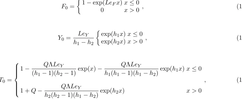
The solution which satisfies the boundary conditions at x→ ±∞ and the jump conditions atx= 0 is
F0 =
1−exp(LeFx)x≤0
0 x >0 , (14)
Y0 =
LeY
h1−h2
exp(h1x)x≤0
exp(h2x)x >0 , (15)
T0=
1− QΛLeY
(h1−1)(h2−1)
exp(x)− QΛLeY
h1(h1−1)(h1−h2)
exp(h1x)x≤0
1 +Q− QΛLeY
h2(h2−1)(h1−h2)
exp(h2x) x >0
, (16)
cf. [14], whereh1 and h2 are the positive and negative roots, respectively, ofh2−LeYh−LeYΛ = 0. The
eigenvalue Λ (and hence the flame speed) is then determined by settingT0 =Tc at x= 0, giving
QΛLeY = (1 +Q−Tc)h2(h2−1)(h1−h2), (17)
which can be straightforwardly solved by Newton-Raphson iteration for Λ. Note that forLeY = 1 equation
(17) has the analytical solution
Λ = Q
2
4(1 +Q−Tc)2
−1
4,
which can be used as an initial guess for non-unity values ofLeY. Note that in any case Λ depends on Q
andTc only through the combination
Q/(1 +Q−Tc) =QD/(QD−1) = (Tad−1)/(Tad −Tc)
[image:7.612.122.472.28.152.2]and does not depend onLeF [14].
Figure 1 shows some example spatial profiles of the steady, planar flame forQ= 5,LeF =LeY = 1 and
[image:7.612.122.540.271.444.2]sheet. The value ofY0at the peak is connected to the crossover temperature, Tc, sinceTad−Tcdetermines
the fraction of the heat still to be released after the fuel has been consumed in the chain-branching reaction sheet, while similarly the peak value of Y0 represents the amount of intermediates still available
for conversion into products (and hence heat). Thus the lowerTcis below the adiabatic flame temperature,
the higher is the peak in the intermediates at x = 0, and hence the further the intermediates are able to diffuse from the reaction sheet. This results in the heat release and hence the temperature rise being spread over a larger distance for lower Tc. On the other hand, asTc→ Tad (or equivalently as QD → 1),
the peak in the radicals becomes very small and thus the fuel is largely converted directly to products. Indeed, it can be shown that in the limitQD →1, the planar flame structure tends to that of the one-step
model (represented as a dotted line in figure 1a) in which intermediates have no role [14].
4 Linearized equations
We now suppose that the steady, planar flame is slightly perturbed such that the perturbed flame position with respect to that of the underlying steady, planar flame is
x=X(y, t), |X(y, t)| 1.
Since the jump conditions (8)-(10) are to be applied on a surface whose position is perturbed, we transform to a frame moving with this perturbed reaction sheet, cf. [9, 19], via
xp=x−X(y, t), yp=y, tp =t, up=u−V(y, t), (18)
where the ‘p’ subscript denotes the perturbed flame co-ordinate system, and
V(y, t) = ∂X
∂t
is the speed of the perturbed reaction sheet in thex-direction. Hence in this new co-ordinate system, the perturbed reaction sheet remains stationary atxp= 0. Note that, under this transformation,∂·/∂x,∂·/∂y,
∂·/∂tare replaced in the governing equations (1)-(6) by
∂·
∂xp
, ∂· ∂yp
−∂X
∂yp
∂·
∂xp
, ∂· ∂tp
−∂X
∂tp
∂·
∂xp
, (19)
respectively, so that∇2 becomes
1 +
∂X ∂yp
2!
∂2·
∂x2
p
+ ∂
2·
∂y2
p
−2∂X
∂yp
∂2·
∂xp∂yp
−∂ 2X
∂y2
p
∂·
∂xp
. (20)
Dold [14] chose to Taylor expand the jump conditions around the x = 0 instead of transforming to the frame of the perturbed flame, the two approaches being equivalent. Henceforth, for convenience we drop the ‘p’ subscript notation.
A normal modes form of the perturbation is then assumed, such that
X(y, t) =eσteiky, <<1, (21)
and the perturbed variables are hence of the form
where q represents any of the dependent variables. Here σ is the (complex) growth rate and k is the wavenumber of the disturbance in the y-direction. For convenience, we define the following quantities in terms of the first derivatives of the perturbations with respect tox:
τ1 =
dT1
dx, U1 =
du1
dx, V1 =
dv1
dx, X1 =F1−
1
LeF
dF1
dx , Z1=Y1−
1
LeY
dY1
dx . (23)
Substituting equations (21)-(23) into the governing equations and linearizing in, gives
du
dx =Au+s, (24)
whereu= (T1, u1, v1, P1, F1, Y1, U1, V1, X1, Z1)T and
A=
(T0 0−σ)
T0
−T0 0
T0
ik 0 0
0 0 0 0 0
0 0 0 0 0
A41 A42
4ikP r(σ+T0−T00)
3T0
0 0
0 0 0 0 LeF
0 0 0 0 0
A71
−σT0
0+T0T000
T2 0
ik(σ+T0−T00)
T0
0 0
0 0 3σ+ 4P rk
2T 0
3P rT0
ik
P r 0
F0 0
T0
−F0 0
T0
0 0 −LeFσ+T0k 2
T0LeF
Y0 0
T0
−Y0 0
T0
0 0 0
0 1 0 0 0
0 1 0 0 0
0 0 1 0 0
−4P rQΛ
3
4P r(σ+T0)−3T0
3T0
−ikP r 0 0
0 0 0 −LeF 0
LeY 0 0 0 −LeY
−QΛ σ+T0
T0
−ik 0 0
0 −ik
3
1
P r 0 0
0 0 0 0 0
−LeYσ−k2T0−LeYΛT0
LeYT0
0 0 0 0
, where
A41=
4P r(−σ2+T0
0σ+k2T02−T0T000)
A42=
−(4P rT0
0+ 3T0)σ
3T2 0
+P r(4T000−3T0k
2)
3T0
−T00
T0
,
A71=
(−σ2+T0
0σ+k2T02−T0T000)
T2 0
,
and
s=
0,0,0,−3σ 2+ 3P
rT0k2σ+PrT0k2T00
3T0
,0,0,−k2T0 0,
ik Pr
−PrT000+T00
,k
2F0 0
LeF
,k
2Y0 0
LeY
T
,
where henceforth a prime denotes differentiation with respect to x. Note that, sinceρ= 1/T, density has been eliminated from equations (1)-(6). Equation (1) then contains only firstx-derivatives of the remaining variables, hence its linearized form has been used to eliminateτ1in terms of the other perturbed quantities:
τ1=
(T0
0−σ)T1
T0
−T00u1
T0
+ ikv1+U1, (25)
Equation (24) is subject to boundedness conditions as x → ±∞. We hence now seek asymptotic so-lutions to equation (24) valid near the fresh or burnt states, as x → ±∞, which can then be used as initial conditions for numerical integration of the equation. In order to obtain higher order terms in these asymptotic solutions, which are necessary for implementation of straightforward shooting methods [12,19], it is beneficial to use one of the steady state solution variables as the independent variable [12, 19]. Given the structure of the steady solution in equations (14)-(16), and given that Y0 → 0 as x → ±∞, here we
choose Y0 as the independent variable for both the fresh and burnt state analyses.
4.1 Asymptotic solution as x→ −∞
Transforming to Y0 as the independent variable by employing equation (15), then in the region x < 0
equation (24) becomes
h1Y0
du dY0
=Au+s, (26)
and the other steady variables can be written in terms ofY0 as
T0 = 1 +α1Y0+β1Y01/h1, F0 = 1 +γ1YLe
F/h1
0 ,
where
α1 =−
QΛ
h1(h1−1)
, β1 =−
QΛLeY
(h1−1)(h2−1)
h1−h2
LeY
1/h1
, γ1 =−
h1−h2
LeY
LeF/h1
.
AsY0 →0,corresponding to x→ −∞, we can thus expand equation (26) in the form
h1Y0
du dY0
= (A0+A1Y0+A2Y01/h1+A3YLe
F/h1
0 +· · ·)u+s0+s1Y0+s2Y01/h1+s3YLe
F/h1
where the co-efficient matrices, A0, etc, depend only on the parametersQ, Pr, LeY, LeF and Tc, and on
σ and k. The homogeneous part of equation (27) has 10 independent asymptotic solutions of the form
u= ˜ui =Y0λi
ai0+ai1Y0+ai2Y 1/h1 0 +ai3Y
LeF/h1
0 +· · ·
, i= 1, . . . ,10, (28)
whereh1λiand ai0 are the eigenvalues and eigenvectors, respectively, ofA0, and theai1,ai2, etc., are found
by substituting (28) into equation (27) and equating powers ofY0. The eigenvalues ofA0 are
±k, 1±[1 + 4(σ+k
2)]1 2
2 ,
1±[1 + 4P r(σ+P rk2)]1 2
2P r ,
LeF ±[Le2F + 4(σLeF +k2)]
1 2
2 ,
LeY ±[Le2Y + 4(σLeY +k2+LeYΛ)]
1 2
2 .
For Re(σ) > 0, the solutions corresponding to the eigenvalues with a negative sign are unbounded as
Y0 → 0 (x → −∞), and hence must be discarded. We are left with 5 linearly independent, bounded, asymptotic solutions, denoted byi= 1, . . . ,5, say.
Equation (26) has an exact particular integral,upL, valid in theentire region to the left ofx = 0,of the form
upL=up0+up1Y0+up2Y 1/h1 0 +u
p
3Y
LeF/h1
0 .
We now therefore have theasymptoticgeneral solution of equation (26), denoted by u˜, valid as Y0 →0 or
x→ −∞, of the form
˜
u=
5
X
i=1
aiu˜i+upL, (29)
whereai are (complex) constants of integration, to be determined.
4.2 Asymptotic solution as x→ ∞
In the regionx >0 equation (24) can be rewritten using Y0 as the independent variable as
h2Y0
du dY0
=Au+s, (30)
and in this region, in terms ofY0, the other steady variables are, from equations (14)-(16),
T0 = 1 +Q+α2Y0, F0 = 0,
where
α2=−
QΛ
h2(h2−1)
,
Asx→ ∞, corresponding to Y0→0, we can therefore expand equation (30) in the form
h2Y0
du dY0
= (A∗
where again the co-efficients matrices,A∗
0, etc, depend only on the parameters and onσ andk. Noting that
in the regionx >0, we must haveF1 =X1 ≡0, the homogeneous part of equation (31) has 8 independent
asymptotic solutions of the form
u= ˆui =Y0λi bi0+bi1Y0+· · ·
, i= 1, . . . ,8, (32)
whereh2λi andbi0 are the eigenvalues and eigenvectors, respectively, of A∗0, and the co-efficients bi1, etc.,
are found by substituting (32) into equation (31) and equating powers ofY0. The eigenvalues of A∗0 are
±k, 1±[1 + 4(σφ+k
2)]1 2
2 ,
1±[1 + 4P r(σφ+P rk2)]12
2P r ,
LeY ±[Le2Y + 4(σφLeY +k2+LeYΛ)]
1 2
2 .
whereφ= 1/(1 +Q) = 1/Tad. For Re(σ) >0, the solutions corresponding to eigenvalues with a positive
sign are unbounded as Y0 → 0 (x → ∞), and again must be discarded. We are thus left with 4 linearly
independent, bounded asymptotic solutions.
Equation (30) has an exact particular integral valid in the regionto the right ofx= 0, upR, of the form
upR=bp0+bp1Y0.
We thus now have the asymptotic general solution,denoted by ˆu, valid as Y0 →0 orx→ ∞, of the form
ˆ
u=
4
X
i=1
biuˆi+upR, (33)
where thebi are (complex) constants of integration, to be determined.
4.3 Jump conditions at x= 0
Upon linearization in , the jump conditions (8)-(10) to be applied at the reaction sheet (x= 0), become
[T1] = [u1] = [v1] = [P1] = [F1] =F1 = [Y1] = 0, (34)
[U1] = [V1] = [X1+Z1] = 0, (35)
T1 = 0. (36)
4.4 Numerical solution of linearized equations
In summary, the linearized problem consists of equation (24) subject to u → u˜ as x → −∞ and u → uˆ asx→ ∞, where ˜u and ˆu are given by equations (29) and (33), respectively, and to the jump conditions (34)-(36) at x= 0.
The numerical solution of the problem is achieved as follows. Firstly, each of the five asymptotic linearly independent solutions, ˜ui, i = 1, . . . ,5 which are valid as x → −∞, are used as initial conditions in the
numerical integration of the homogeneous form of equation (24), starting from a sufficiently large negative value ofx (corresponding to a small value of Y0), up to x= 0. A fourth-order Runge-Kutta routine with
region left ofx= 0. Hence the general solution in this region,uL, is of the form
uL=
5
X
i=1
aiuiL+upL.
In particular, we can now evaluate numerically the general solution at x = 0 reached from the left, i.e.
uL(x= 0).
Similarly, the four asymptotic linearly independent solutions, ˆui, i = 1, . . . ,4, can be used as initial
conditions for numerical integration of the homogeneous part of equation (24) back tox= 0 starting from a sufficiently large value of x. This gives numerically the four bounded linearly independent solutions in the entire region to the right ofx= 0, denoted byuiR,i= 1, . . . ,4. The general solution forx >0 is hence of the form
u=uR=
4
X
i=1
biuiR+upR,
from whichuR(x= 0) can be evaluated.
It remains to determine the (complex) constants of integration, ai and bi. These are chosen so as to
satisfy the jump conditions (34)-(35). Given the form of these jump conditions, we define a new reduced set of dependent variables byq= (T1, u1, v1, P1, F1, Y1, U1, V1, X1+Z1)T, which is hence straightforwardly
constructed by adding the ninth and tenth entries of u. The jump conditions (34) and (35) can thus be written in the form
qL(x= 0) =qR(x= 0), (37)
where qL and qR are just the reduced versions of uL and uR, respectively. This is a system of 9
simul-taneous linear equations for the 9 constants of integration, a1 to a5 and b1 to b4. These can hence be
straightforwardly determined for given parameters such that the conditions (37) are satisfied.
However, determining the constants of integration in this manner also fixes the value of T1 at x = 0.
Only for certain discrete values ofσ (for fixedk) will the condition (36) be simultaneously satisfied. The eigenvalues are hence found by Newton-Raphson iteration on the condition T1 = 0. Note that, for fixed
parameters, equation (24) and the boundary and jump condition do not have any leading order dependence on the activation energy of the chain-branching step, unlike for the one-step model whenLeF is fixed [9].
5 Linear stability results
As for the one-step Reactive Navier-Stokes model [9] and for the two-step CDM [14], we find there are only two possible distinct modes. The first of these is a cellular mode for whichσ is real, and the second a pulsating mode corresponding to a complex conjugate pair of eigenvalues. In this section, the linear neutral stability boundaries and linear dispersion relations of the two-step branching flame are examined for both these cellular and pulsating branches, when thermal expansion is taken into account. The effect of the various model parameters is explored, and the results compared and contrasted with both the two-step CDM predictions and the Reactive Navier-Stokes one-step chemistry results.
5.1 Effect of thermal expansion and comparison with CDM
We first examine the effect of varying thermal expansion (through the heat of reactionQ) on the stability of the flame. For the two-step CDM, in which hydrodynamical effects induced by thermal expansion are completely ignored, the linear stability is independent ofQfor fixed values ofQD =Q/(Tc−1) [14]. Since
0 0.2 0.4 0.6 0.8 1
1.8 1.5 1.2 0.9 0.6 0.3
k
LeF
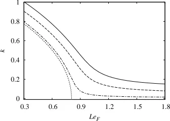
Figure 2. Neutral stability boundary of the cellular branch in theLeF−kplane forLeY = 1 andQD= 1.25 (Tc= 1 +Q/1.25), when
Q= 5 (Tc= 5) (solid line),Q= 1 (Tc= 1.8) (dashed line) andQ= 0.1 (Tc= 1.08) (dot-dashed line). Dotted line is the CDM prediction forQD= 1.25.
consistent to first examine the stability effect of varyingQwhile keeping QD fixed (and hence varyingTc
appropriately).
5.1.1 Cellular branch. Figure 2 shows the neutral stability boundaries in theLeF−k plane for various
values of Q when QD = 5/4 (hence Tc = 1 + 4Q/5) and LeY = 1. These neutral stability boundaries
correspond to the loci on which σ = 0, and the flame is unstable to wavenumbers below the curve and stable to those above it. The dotted curve in figure 2 is the neutral stability boundary for QD = 5/4 as
predicted by the two-step CDM. The CDM results predicts the flame is stable to all wavenumbers above a critical fuel Lewis number, while as LeF decreases below this critical value the flame becomes unstable
to an increasingly wide band of wavenumbers [14]. Since the CDM ignores hydrodynamic effects, the instability predicted by the CDM is of a purely thermal-diffusive natures. However, the two-step Reactive Navier-Stokes model studied here simultaneously captures hydrodynamic effects, and figure 2 shows that the stability results are then qualitatively different to the predictions of the CDM, even whenQ is quite small. In particular the flame is unstable for all values of LeF, at least for sufficiently long wavelength
perturbations. While the CDM is valid in the asymptotic limit Q→0, figure 2 also shows that even for a physically very small heat release of Q= 0.1, this hydrodynamical effect is still important. Hence, while theQ= 0.1 stability boundary follows closely that of the CDM for fuel Lewis numbers sufficiently below the criticalLeF predicted by the CDM, it then curves sharply to the right near this critical value. Hence
the concept of anLeF stability boundary predicted by the CDM is not physically valid for gaseous flames.
A second difference is that, while the CDM results are independent of Q for fixed QD, figure 2 shows
that when hydrodynamic effects are taken into account, the stability does depend onQ (with QD fixed).
Indeed, the higher the value ofQ, the wider the range of unstable wavenumbers for any fixedLeF, so that
the neutral stability curve for a given Q lies above those corresponding to lower values in the LeF −k
plane.
For the cellular instability, a larger value of the neutrally stable wavenumber also corresponds to a more unstable flame, in that the maximum linear growth rate is also larger. This is demonstrated in figure 3, which shows the dispersion relations (growth rate,σ, as a function of wavenumber,k) for various values of
QwhenLeF = 0.6 and whenLeF = 1.2. Note, for the cellular mode,σis also zero atk= 0. AsQincreases,
not only does the band of unstable wavenumbers increase for fixedLeF, but so does the wavenumber with
the maximum value of the growth rate, and the value of this maximum also rapidly increases. Thus weak perturbations to the planar flame will grow much more rapidly and become non-linear more quickly for largerQ. One would expect that cells would first appear on the flame with a wavenumber close to that with maximum linear growth rate. However, it should be noted that a linear analysis only gives information about stability boundaries, onset and initial growth stage of the instability. It is not relevant to the fully developed non-linear cells, which may be of a quite different characteristic wavelength to that predicted by the linear analysis [13].
The dependence of the cellular instability on Q, with fixed QD, described above is qualitatively the
[image:14.612.214.382.29.149.2]0.5
0.4
0.3
0.2
0.1
0
0.8 0.6
0.4 0.2
0
σ
k
(a) 0.08
0.06
0.04
0.02
0
0 0.05 0.1 0.15 0.2 0.25
σ
k
(b)
Figure 3. Dispersion relations of the cellular instability forLeY = 1,QD= 1.25 and (a)LeF = 0.6 and (b)LeF = 1.2, whenQ= 5 (Tc= 5) (solid line),Q= 1 (Tc= 1.8) (dashed line) andQ= 0.1 (Tc= 1.08) (dot-dashed line). Dotted line in (a) is the CDM
prediction forQD= 1.25.
0 0.2 0.4 0.6 0.8 1
1.8 1.5 1.2 0.9 0.6 0.3
k
LeF
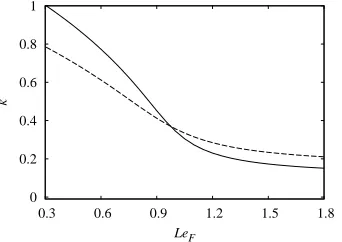
Figure 4. Neutral stability boundary of the cellular branch in theLeF−kplane forLeY = 1,Tc= 5 andQ= 5 (QD= 1.25) (solid line) andQ= 6 (QD= 1.5) (dashed line).
and Reactive Navier-Stokes model predictions are also qualitatively the same in the one-step case, cf. Jackson and Kapila [9]. For the two-step model, however, the effect of varyingQbut keeping the crossover temperature,Tc, fixed is somewhat more complicated. Figure 4 shows the neutral stability boundaries for
Tc= 5 and heats of reactionQ= 5 and 6 (corresponding toQD = 1.25 and 1.5, respectively). The stability
response of the flame with the larger thermal expansion is less sensitive to the fuel Lewis number than for the smaller Q case. The neutral stability curves for the two thermal expansions cross in the LeF −k
plane, in this case atLeF = 0.97, and the flame is more (less) unstable for the smaller degree of thermal
expansion when LeF is above (below) this value. Thus, for LeF sufficiently below unity, the stabilizing
effect of decreasing thermal expansion is outweighed by a destabilizing thermal-diffusive effect as QD is
lowered by the increase inQ (cf.§5.2.1).
5.1.2 Pulsating branch. Recall that the pulsating instability branch corresponds to a complex conjugate pair of eigenvalues. For the CDM limit, this instability is found to occur only providedQD is below a finite
value, and then only ifLeF is above a critical value which is greater than unity [14]. This critical value of
the fuel Lewis number decreases and tends to unity asQD →1. However,QD−1 still has to be sufficiently
small for the pulsating instability to occur for values ofLeF realistic to gaseous flames. For example, figure
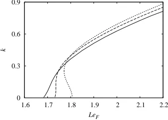
5 shows the CDM prediction of the neutral stability boundary whenQD−1 = 0.1 (forLeY = 1), in which
caseLeF needs to be above 1.772 for the flame to be unstable to the pulsating mode. Note that the CDM
predicts that the pulsating instability first appears at an non-zero wavenumber [14]. For example, when
QD = 1.1, the wavenumber is 0.252 at the turning point of the CDM neutral stability curve in figure 5.
Figure 5 also shows the neutral stability boundaries, on which Re(σ) = 0, predicted by the Reactive Navier-Stokes model with O(1) values of the thermal expansion, but with QD = 1.1 fixed. As for the
CDM prediction, when hydrodynamic effects are taken into account, the pulsating instability still only occurs above a critical value ofLeF. Increasing thermal expansion lowers this critical value somewhat. For
[image:15.612.124.474.29.151.2] [image:15.612.215.386.207.328.2]0.9
0.6
0.3
0
1.6 1.7 1.8 1.9 2 2.1 2.2
k
LeF
Figure 5. Neutral stability boundary of the pulsating branch in theLeF−kplane forLeY = 1 andQD= 1.1 (Tc= 1 +Q/1.1) when
Q= 5 (Tc= 5.545) (solid line) andQ= 1 (Tc= 1.909) (dashed line). Dotted line is the CDM prediction forQD= 1.1.
0.6
0.4
0.2
0
0.4 0.3
0.2 0.1
0
Re( )
k
(a)
σ
5
4
3
2
1
0
0.4 0.3
0.2 0.1
0
Im( )
k
(b)
σ
Figure 6. Dispersion relation ((a) growth rate and (b) frequency) of the pulsating instability forLeY = 1,LeF = 1.8,QD= 1.1,Q= 5 (Tc= 5.545) (solid line) andQ= 1 (Tc= 1.909) (dashed line). Dotted line is the CDM prediction forQD= 1.25.
5, as compared to the CDM prediction of LeF >1.772. Also, in contrast to the CDM prediction, there is
no turning point in the neutral stability boundary when hydrodynamic effects are taken into account, i.e. the instability first occurs at zero wavenumber.
Figure 5 also shows that for Lewis numbers of the fuel above the CDM critical value, thermal expansion only has a weak effect on the neutral stability boundary. In this region, the boundary for larger values of Q actually lie below those corresponding to lower values, and hence also below the CDM prediction. This weak dependence of the pulsating instability boundary on thermal expansion, for fixed QD, is again
qualitatively the same as the effect ofQon the boundaries in the one-step model [9].
It is important to note, however, that for the pulsating branch, the range of unstable wavenumbers does not relate to the degree of instability of the wave. Hence, although thermal expansion has only a weak effect on the stability boundaries, it has a large effect on the actual dispersion relations (growth rate,
Re(σ), and frequency,Im(σ), versus wavenumber) as shown, for example, in figure 6. Furthermore, while the CDM predicts that the maximum growth rate occurs at a non-zero wavenumber (hence the turning point in the CDM neutral stability curve), forO(1) values of Q, the maximum growth rate occurs atk= 0 (infinite wavelength). This corresponds to a purely one-dimensional pulsation of the planar flame being the linearly most unstable mode. The growth rate atk = 0, and hence the degree of instability, also increases quite rapidly with Q, even though the range of unstable wavenumbers decreases. The frequency of the pulsation also increases withQ, and hence the period, given by 2π/Im(σ), decreases.
5.2 Effect of crossover temperature and comparison with one-step model
The two-step CDM results predict that as Tc→Tad, the flame becomes increasingly unstable in that the
critical values ofLeF at which the cellular and pulsating instability occurs both tend to unity [14]. In this
[image:16.612.213.382.29.150.2] [image:16.612.122.474.198.322.2]1.6
1.2
0.8
0.4
0
1.8 1.5 1.2 0.9 0.6 0.3
k
LeF
(a) 1.2
0.9
0.6
0.3
0
-10 -5 0 5 10
k
l
(b)
Figure 7. Neutral stability boundary of the cellular branch (a) in theLeF−kplane and (b) in thel−kplane (l=βeff(LeF −1),
βeff= 2QD/(QD−1)), forQ= 5,LeY = 1 andTc= 4 (QD= 5/3,βeff= 5) (solid lines),Tc= 5 (QD= 1.25,βeff= 10) (dashed lines) andTc= 5.7 (QD= 1.064,βeff= 33.333) (dotted lines). Also shown in (b) is the high-activation energy one-step model result from
Jackson and Kapila [9] (dot-dashed line)
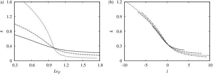
5.2.1 Cellular branch. Figure 7(a) shows the neutral stability boundary when Q = 5 for various Tc
(and hence varying QD also), when LeY = 1. Again, when thermal expansion is taken into account, the
flame is unstable to the cellular instability for all values of LeF, and there is no critical Lewis number
as in the CDM prediction. For unit values ofLeF and LeY and realistic thermal expansions, the cellular
instability is insensitive to Tc. Thus the neutral stability curves for the different values of Tc cross at
LeF = 1 in figure 7(a). AsTc→Tad (or equivalently asQD →1) the flame becomes increasingly sensitive
to thermal-diffusive effects associated with the Lewis number of the fuel. These effects are destabilizing when LeF <1, but stabilizing for LeF >1, and appear to have an enhanced role as QD → 1. Thus, for
fixed values ofLeF which are less than unity, the flame becomes increasingly unstable (the neutrally stable
wavenumber becomes larger) asTcincreases. Conversely, for fixed values ofLeF >1, the thermal-diffusive
effect becomes more strongly stabilizing, and hence the neutrally stable wavenumber decreases.
These dependences of the cellular mode stability boundaries in the LeF −k plane on Tc are in fact
qualitatively similar to the dependence of the one-step model boundaries on activation energy [12]. Indeed, in the high-activation energy asymptotic limit, the one-step flame stability depends on LeF and the
activation energy only through a reduced Lewis number, l, defined by l = β(LeF −1) [9], such that
l=O(1) asβ → ∞(i.e. the NEF approximation), whereβ is the Zel’dovich number (thenon-dimensional
activation energy of the one-step reaction rate). Dold [14] showed that, for the constant density models, in the limit Tc → Tad there is a direct correspondence between the flame structure and stability of the
one-step and two-step chemistry models. Indeed, under the asymptotic limitQD →1, the two-step model
can be described to leading order by a one-step model which has aneffectiveZel’dovich number defined by
βeff = 2QD/(QD−1) = 2(Tad−1)/(Tad−Tc). In other words, in the limit, the two-step CDM linear stability
depends to leading order onLeF only through a reduced Lewis number defined by l=βeff(LeF −1), and
this leading order dependence is then the same to that of the one-step model with Zel’dovich number
β=βeff [14].
Since the analysis in Dold [14] is based on comparing the two-step jump conditions in the temperature and fuel in the limitQD →1 with those of the one-step model, and these jump conditions are unchanged
when thermal expansion is taken into account, one would expect the analogy between the two models to still hold in the Reactive Navier-Stokes formulation. However, it remains to determine how predictive the one-step model is of the two-step results for non-zero values of QD −1 (finite βeff) when thermal
expansion is taken account of. Figure 7(b) shows the neutral stability boundaries in the reduced Lewis number-wavenumber (l−k) plane, when Q = 5, for Tc = 4 (corresponding to QD = 1.667, βeff = 5),
Tc= 5 (QD = 1.25,βeff = 10) andTc= 5.7 (QD = 1.064,βeff = 33.333). Also shown is the one-step model
high activation energy result for Q = 5 from Jackson and Kapila [9]. It can be seen that, in this plane, the stability boundary is only weakly dependent onTc, and the chain-branching model results do converge
to those of one-step model as QD → 1. Furthermore, the prediction of the one-step model remains quite
good even whenQD−1 is of the order of unity, or βeff is moderately large. However, it is important to
[image:17.612.124.474.28.151.2]0.8
0.6
0.4
0.2
0
2.2 2
1.8 1.6
1.4
k
LeF
(a) 0.8
0.6
0.4
0.2
0
10 12 14 16 18 20 22
k
l
(b)
Figure 8. Neutral stability boundary of the pulsating branch (a) in theLeF−kplane and (b) in thel−kplane forQ= 5,LeY = 1 andTc= 5.545 (QD= 1.1,βeff= 22) (solid lines),Tc= 5.6 (QD= 1.087,βeff= 25) (dashed lines) andTc= 5.65 (QD= 1.075,
βeff= 28.57) (dotted lines). Also shown in (b) is the high-activation energy one-step model result from Jackson and Kapila [9] (dot-dashed line)
chain-branching step), but is a function of the the crossover temperature [14]. In particular, βeff can be
arbitrarily large compared to any physical Zel’dovich number.
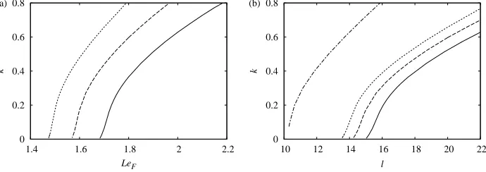
5.2.2 Pulsating branch. Figure 8(a) shows the neutral stability curves of the pulsating branch for various values of Tc, when Q = 5 and LeY = 1. Unsurprisingly, since thermal expansion has a weak
effect on the pulsating instability boundary, the dependence onTc (and hence on QD) follows the trends
predicted by the CDM [14], i.e. the critical value ofLeF decreases towards unity withQD. The dependence
of the neutral stability curves in thel−kplane is more interesting. Figure 8(b) shows the neutral stability boundaries in this plane, together with the one-step boundary for the pulsating branch whenQ= 5 from Jackson and Kapila [9]. The values of Tc used in figure 8 correspond to βeff = 22, 25 and 28.57. The
stability of the pulsating branch in the l−k plane can be seen to be much more sensitive to βeff than is
the cellular instability (cf figure 7(b)). Furthermore, while the two-step model results do tend to those of the one-step model as βeff → ∞(Tc→Tad), it is apparent that a very high βeff would be required for the
one-step and two-step model results to quantitatively agree.
Interestingly, these effects of finiteβeff on the two-step model pulsating instability boundary in thel−k
plane are actually very similar to the role of finite activation energy in the one-step model. Lasseigne et al.[10] performed a numerical linear stability analysis of the one-step reaction CDM with finite activation energy (i.e. without invoking the high activation energy asymptotic limit). They also found that, for the pulsating instability, the results are sensitive to β, with the finite activation energy results lying further to the right in thel−k plane the lower the Zel’dovich number, and that a very largeβ would be required for the high-activation energy asymptotic one-step theory to be quantitatively predictive.
5.3 Effect of Lewis number of intermediates.
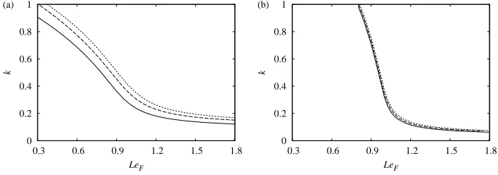
Figure 9 shows the stability boundaries of the cellular mode for various values of the intermediates Lewis number for Q = 5 when Tc = 5 and when Tc = 5.7. Increasing LeY can be seen to have a destabilizing
effect on the cellular mode, in that the neutral stability curves for higher LeY lie entirely above those of
lower values. However, figure 9 also shows that the destabilizing effect becomes weaker as Tc increases,
and the results becomes independent of LeY in the limit QD → 1. This is to be expected, since as Tc
tends to Tad, the amount of intermediates, and hence the role of their diffusion in the flame structure,
decreases (see figure 1). For the pulsating branch, however, increasing LeY is found to have a stabilizing
effect, in that the critical fuel Lewis number for this instability becomes larger as LeY increases, cf. the
CDM prediction [14]. The dependence of the pulsating branch critical fuel Lewis number on LeY again
[image:18.612.126.471.29.151.2]0 0.2 0.4 0.6 0.8 1
1.8 1.5 1.2 0.9 0.6 0.3
k
LeF
(a)
0 0.2 0.4 0.6 0.8 1
1.8 1.5 1.2 0.9 0.6 0.3
k
LeF
(b)
Figure 9. Neutral stability boundary of the cellular branch in theLeF−kplane forQ= 5 and (a)Tc= 5 and (b)Tc= 5.7, when
LeY = 0.3 (solid lines),LeY = 1 (dashed lines) andLeY = 1.8 (dotted lines)
6 Conclusions
A leading order, high-activation energy asymptotic linear stability analysis of premixed flames has been performed in the context of a two-step chain-branching chemistry, Reactive Navier-Stokes model. The main purpose was to extend the results of a previous study, which employed a constant density model [14], to take into account hydrodynamic effects induced by thermal-expansion. The main difference is that, as found previously for the standard one-step chemistry model, when thermal expansion is taken into account, the flame always has a band of perturbation wavelengths which are unstable to a cellular mode. Hence the region of stable fuel Lewis numbers predicted by the constant density study does not exist for realistic thermal expansions. On the other hand, a sufficiently large, critical fuel Lewis number is still required for the flame to be unstable to a pulsating mode, as correctly predicted by the constant density model. For this mode, thermal expansion has a weak effect on the stability boundaries, but a large effect on the maximum linear growth rate.
Comparing the results with those of a previous one-step reaction Reactive Navier-Stokes study [9], the two-step behaviour is found to be broadly similar, and hence no qualitatively new behaviour is revealed by using the more realistic two-step model. Furthermore, in the limit that the branching cross-over tem-perature, Tc, tends to the adiabatic flame temperature,Tad, the two-step model results can be identified
to leading order with those of a one-step model with a suitably defined effective activation energy. This effective activation energy tends to infinity in the limit Tc →Tad, and hence unlike a physical activation
energy, can be arbitrarily large. The one-step model approximation is found to be quantitatively good for the cellular instability even when the effective activation energy is moderately large. For the pulsating instability, however, it is found that a crossover temperature very close to the adiabatic temperature (cor-responding to a very large effective activation energy) would be required for the effective one-step results to be quantitatively predictive of the two-step model results.
Here we have considered adiabatic, freely propagating premixed flames. Secondary effects, such as buoy-ancy, heat loss, endothermic branching reaction, finite activation energy effects, etc., could also be included in future linear stability studies. However, calculations of the fully non-linear stages of the evolution, and studies of how these compare and contrast to the fully non-linear one-step model results, would perhaps be a more important next step. Direct numerical simulations using the two-step model, along the lines of the one-step computations in Sharpe and Falle [13], will be presented in a future article.
Acknowledgments
[image:19.612.121.473.28.152.2]References
[1] Buckmaster, J. D. and Ludford, G. S. S., 1982,Theory of Laminar Flames.Cambridge University Press.
[2] Sivashinsky, G. I., 1983, Instabilities, pattern formation, and turbulence in flames.Ann. Rev. Fluid Mech.,15, 179–199.
[3] Strehlow, R. A., 1985,Combustion Fundamentals.McGraw-Hill. [4] Law, C. K., 2006,Combustion Physics.Cambridge University Press.
[5] Sivashinsky, G. I., 1977, Diffusional-thermal theory of cellular flames.Combust. Sci. Tech.,15, 137–146.
[6] Frankel, M. L. and Sivashinsky, G. I., 1982, The effect of viscosity on hydrodynamic stability of a plane flame front.Combust. Science Tech.,29, 207–224.
[7] Matalon, M. and Matkowsky, B. J., 1982, Flames as gasdynamic discontinuities.J. Fluid Mech.,124, 239–259.
[8] Pelce, P. and Clavin, P., 1982, Influence of hydrodynamics and diffusion upon the stability limits of laminar premixed flames.J. Fluid Mech.,124, 219–237.
[9] Jackson, T. L. and Kapila, A. K., 1984, Effect of thermal expansion on the stability of plane, freely propagating flame.Combust. Science Tech.,41, 191–201.
[10] Lasseigne, D. S., Jackson, T. L. and Jameson, L., 1999, Stability of freely propagating flames revisited.Combust. Theory Model.,3,
591-611.
[11] Liberman, M. A., Bychkov, V. V., Goldberg, S. M. and Book, D. L., 1994, Stability of a planar flame front in the slow-combustion regime.Physical Review E,49, 445–453.
[12] Sharpe, G. J., 2003, Linear stability of planar premixed flames: Reactive Navier-Stokes equations with finite activation energy and arbitrary Lewis number.Combust. Theory Model.,7, 45–65.
[13] Sharpe, G. J. and Falle, S. A. E. G., 2006, Nonlinear cellular instability of planar premixed flames: numerical simulations of the Reactive Navier-Stokes equations. Combust. Theory Model.,10, 483-514.
[14] Dold, J. W., 2007, Premixed flames modelled with thermally sensitive intermediate branching kineticsCombust. Theory Model.,in press (available in online edition at http://www.tandf.co.uk/journals/titles/13647830.asp).
[15] Dold, J. W., Thatcher, R. W., Omon-Arancibia, A. and Redman, J., 2003, From one-step to chain-branching premixed-flame asymptotics.Proc. Combust. Inst.,291519–1526.
[16] Dold, J. W., Weber, R.O., Thatcher, R. W., Shah, A. A., 2003, Flame balls with thermally sensitive intermediate kinetics.Combust. Theory Model.,7, 175–203.
[17] Williams, F. A., 1985,Combustion Theory,2nd Ed. Addison-Wesley Publishing.
[18] Gasser, I. and Szmolyan, P., 1995, Detonation and deflagration waves with multistep reaction schemes.SIAM J. Appl. Math.,55,
175–191.