Modelling the population dynamics of a benthic octopus species : exploring the potential impact of environment variation and climate change

Modelling the population

dynamics of a benthic

octopus species: exploring

the potential impact of

environment variation and

climate change

by

Jessica André (MSc)

Submitted in fulfilment of the requirements for the degree of

Doctor of Philosophy in Quantative Marine Science

School of Zoology

University of Tasmania

Frontispiece: fractal “Electric octopus”

Declarations

Statement of originality

This thesis contains no material that has been accepted for a degree or diploma by the University or any other institution. To the best of my knowledge and belief, this thesis contains no material previously published or written by another person, except where due acknowledgement is made in the text, nor does the thesis contain any material that infringes copyright.

Jessica André ____________________ Date _____________________

Statement of authority of access

This thesis may be available for loan and limited copying in accordance with the Copyright Act 1968.

Abstract

Cephalopods are increasingly targeted by fisheries, yet their population dynamics are generally poorly understood due to their intrinsically complex nature and their great sensitivity to environmental factors. As a consequence, population structure and biomass can change rapidly over short time-scales, with currently no means of predicting future recruitment or the consequences of climate change on these species. The aim of this study was therefore to develop a mechanistic model to predict the population dynamics and the potential impact of environmental variability and climate change on a cephalopod species.

on the growth threshold at which the switch from fast to slower growth occurs. In order to simulate juvenile growth trajectories in the wild, the bioenergetic model was further developed to include dynamic seasonal temperatures and individual variability in growth and hatching size. Results indicated that hatching size was secondary to inherent variation in growth rates in explaining size-at-age-differences, and that size-at-age distributions in some cohorts tended to become bimodal under certain food intake levels. Predictions from the individual-based bioenergetic models were integrated into a matrix population model, which was used to project the population under the predicted temperature conditions generated by the Commonwealth Scientific and Industrial Research Organisation (CSIRO) from the emission scenarios of the Intergovernmental Panel for Climate Change (IPCC). Simulations suggested that increasing water temperatures might not be as beneficial to octopus as previously thought. Survivorship and incubation time were found to drive the population dynamics and while O. pallidus has the potential to survive under climate change conditions, the population structure and dynamics are likely to change substantially with a potential decrease in average generation time, a streamlining of the life cycle, and a possible loss of resilience to catastrophic events.

Statement of co-authorship

Chapters 2-4 of this thesis have been prepared as scientific manuscripts as identified on the title page for each chapter. In all cases experimental design and implementation of the research program, modeling, data analysis, interpretation of results and manuscript preparation were the primary responsibility of the candidate, but were carried out in consultation with supervisors, and with the assistance of co-workers. Contributions of co-authors and co-workers are outlined below:

Chapter 2:

• Dr Gretta Pecl (Tasmanian Aquaculture and Fisheries Institute (TAFI)) is the primary supervisor for this PhD and provided advice on the experimental design and analyses of the results, as well as manuscript preparation.

• Dr Jayson Semmens (TAFI) is a supervisor for this PhD and provided advice on the biology of Octopus pallidus, as well as the experimental design and maintenance of octopus for the laboratory experiment and manuscript preparation.

Chapter 3:

• Dr Eric Grist (UHI Millenium Institute) provided advice on the modeling approach, data analyses and interpretation of results as well as manuscript preparation.

• Dr Gretta Pecl (TAFI) provided advice on cephalopod biology and physiology, and manuscript preparation.

• Dr Jayson Semmens (TAFI) provided guidance on octopus biology, specifically on octopus growth, and manuscript preparation.

• Prof Susumu Segawa (Tokyo Univeristy of Marine Science and Technology) is a collaborator and provided the experimental data sets for

Octopus ocellatus

Chapter 4:

• Dr Gretta Pecl (TAFI) provided guidance in the areas of cephalopod biology and ecology, as well as interpretation of the results and manuscript preparation.

• Dr Eric Grist (UHI Millenium Institute) provided advice on the modeling approach and manuscript preparation.

• Dr Jayson Semmens (TAFI) provided advice on the interpretation of the results and manuscript preparation.

• Stephen Leporati (TAFI) is a collaborator and provided the size-at-age datasets for wild Octopus pallidus.

Chapter 5:

• Prof Malcolm Haddon (CSIRO) provided guidance on the modeling approach and statistical interpretation of the results, as well as manuscript preparation.

• Dr Gretta Pecl (TAFI) provided advice in the areas of cephalopod biology and ecology, specifically on possible implications of climate change, as well as manuscript preparation.

• Stephen Leporati (TAFI) provided the fecundity dataset for wild Octopus pallidus.

Acknowledgments

My supervisors, Gretta Pecl, Jayson Semmens, Eric Grist and Malcolm Haddon have been fantastic mentors throughout this PhD. I thank Gretta and Jayson for their guidance, encouragement and support throughout this project, and for understanding the tribulations of doing a PhD with a young child. I thank Eric for teaching me about modeling and rational thinking, and for giving me the opportunity to see Cambridge and walk in Newton’s steps (literally…). I thank Malcolm for providing help in times of need, both before and during his time as a supervisor, and for making statistics not so repulsive... Thank you to all the members of TAFI for providing an excellent working environment, and special thanks to those who have contributed time and advice at some point or another during this project: Phillipe Ziegler, Sean Tracy, Alan Beech, Bill Wilkinson, Sam Foster, Bob Hogston, Vanessa Lucieer, Mike Poteus and Ed Smith. I also would like to thank Professor Segawa san for sharing his raw data on

Octopus ocellatus, which allowed me to fully test my models, and Dr Alistair Hobday for providing access to climate change predictions for the Bass Strait region.

members of the cephalopod student team: Zoë Doubleday for the laughs and for putting up with my organised mess in the office; and Stephen Leporati: for his friendship and support since the beginning of this PhD (including sharing his hard earned dataset on wild octopus). Cursing the temperamental heater/chiller and hunting ghost crabs for our hoards of hungry octopus would not have been as much fun without you…

I would like to thank my family, for their enduring love, for never doubting me and supporting me throughout the years. A special thanks to the two men in my life: my partner, Peter-Johannes Pfeiffer, and my son, Niels. We have come a long way, sailed through the stormy waters and pulled through stronger. You have brought out the best (and sometimes the worst…) in me. Weil I eich mog.

And finally, I would like to share this haiku about the art of biological modelling, written in a moment of disillusionment:

Sometimes they work fine

Yet most times they crap themselves

Contents

Declarations i

Abstract ii

Statement of co-authorship

iv

Acknowlegments vii

List of Figures

xiv

List of Tables

xxiii

List of Equations

xxv

Ch. 1 General Introduction

1

CEPHALOPODS: ROLE AND CHARACTERISTICS 2

PLASTICITY AND POPULATION DYNAMICS 4

CEPHALOPODS AND CLIMATE CHANGE 8

AIMS AND THESIS STRUCTURE 12

STUDY SPECIES 16

Octopus pallidus (Hoyle 1885) 16

Octopus ocellatus (Gray 1849) 17

Ch. 2 The early life-history processes: relationships between

temperature, feeding, food conversion and growth

19

ABSTRACT 20

INTRODUCTION 21

MATERIAL AND METHODS 23

Study animals and experimental design 23 Growth, food consumption, and food conversion rate 25

Data analysis 28

RESULTS 30

Food consumption, food conversion rate, and growth rate 31 Effect of temperature on Fr, Gr and Cr 37

Feeding rate and growth rate 39

Feeding rate and food conversion rate 40 Growth rate and food conversion rate 42

DISCUSSION 44

Food consumption, food conversion rate and growth rate 44 Effect of temperature on Fr, Gr and Cr 45

Relationship between Fr, Gr and Cr 46

CONCLUSION 49

Ch. 3 Modeling the impact of temperature on the growth

pattern of octopus using bioenergetics

50

INTRODUCTION 52

THE ENERGY BALANCE MODEL 54

Concept 54 Incorporation of temperature dependency: the temperature-dependent energy balance model (TEBM) 57

METHODS 57

Data sets 59

Experimental estimation of p2 for O. pallidus 60 Experimental estimation of transition body mass and age 63

Model parameterisation 64

Model estimation of transition body mass and age 73

Sensitivity analysis 74

RESULTS 74

Estimation of transition body mass and age 74 Impact of temperature on growth pattern 75

Model sensitivity 77

DISCUSSION 79

CONCLUSION 82

Ch. 4 Modeling size at age in wild immature octopus: the

relative influence of the pricipal abiotic and biotic factors 84

INTRODUCTION 86

Dataset 91

Model development 92

Simulation 105

RESULTS 108

Estimation of growth and feeding parameters for wild caught octopus 108 Projected size-at-age at 60, 90 and 120 days 110 Projected age at sexual maturity 112 Relative influence of hatchling size and inherent growth capacity

on size-at-age 112

Projected influence of food intake on size-at-age 113 Projected influence of food intake on age at sexual maturity 116

DISCUSSION 116

CONCLUSION 123

Ch. 5 Predicted effect of climate change on the western Bass

Strait pale octopus population

124

METHODS 129

General form of the model 129

Bioenergetics model 132

Matrix population model 144

Simulations and model analyses 150

RESULTS 152

Elasticity analyses 167

DISCUSSION 168

CONCLUSION 176

Ch. 6 General discussion

177

GENERAL DISCUSSION 178

APPLICABILITY TO OTHER SPECIES AND FUTURE STUDIES 188

References 193

List of Figures

Fig. 1.1 Global landing of cephalopods from 1950 to 2005. Data include commercial, industrial, recreational and subsistence purpose catches (sourced from the FAO Global Production Statistics)... 3

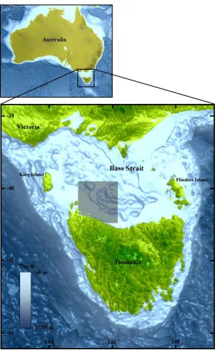
Fig. 1.2 Map of the study area. The grey square represents the location of the O. pallidus population from this study... 13

Fig. 1.3. Distribution of pale octopus Octopus pallidus and gold-spot octopus Octopus ocellatus. Photos courtesy of Kobe Municipal Suma Seaside Aquarium and Kay (O. ocellatus), and Harry Wright (adult O. pallidus)... 18

Fig. 2.1 Intended ( --- ) and actual ( ─ ) temperature regimes recorded during the experiment. Standardised (std) temperature used in the time series analysis (see Data analysis section p. 28)are represented by circles for the cool regime and squares for the warm regime... 24

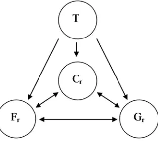
Fig. 2.2 Schematic diagram of the relationships between temperature T, feeding rate Fr, growth rate Gr and food conversion Cr investigated in this chapter... 29

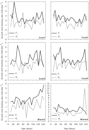
Fig. 2.3 Standardised feeding rate Fr and growth rate Gr (in % body weight per day) experienced by individual octopus. Note the change of scale for Warm4... 32

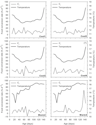
Fig. 2.5 Standardised food conversion rate Cr (in % per day) and temperature experienced by individual octopus. It was not possible to calculate Cr between day 136 and day 143 for Cool4. ... 34

Fig. 2.6 a) Autocorrelation plot of food conversion rate for Warm2; b) autocorrelation plot of growth rate for Cool4. Bars that protrude beyond the dotted lines indicate significant correlations. ... 35

Fig. 2.7 Raw data of individual (─) and average (---) growth under the a) cool and b) warm temperature regime... 36

Fig. 2.8 Cross- correlation plots showing the influence of temperature T on feeding rate Fr, growth rate Gr and food conversion rate Cr: a) T on the mean Cr for the cool regime; b) T on Cr for individual Cool4; c) T on the mean Fr for the cool regime; d) T on the mean Fr for the warm regime; e) T

on the mean Gr for the cool regime; f) T on the mean Gr for the warm regime. Bars that protrude beyond the dotted lines indicate significant correlations. ... 38

Fig. 2.9 Cross-correlation plots showing the relationship between feeding rate Fr and growth rate Gr: a) mean Fr on mean Gr for the cool regime; b) mean Fr on mean Gr for the warm regime; c) mean Gr on mean Fr for the warm regime; d) Gr on Fr for Warm2. Bars that protrude beyond the dotted lines indicate significant correlations... 39

Fig. 2.10 Cross-correlation plots showing the relationship between food conversion rate Cr and feeding rate Fr: a) mean Cr on mean Fr for the cool regime; b) Cr on Fr for Cool3; c) Cr on Fr for Cool4; d) mean Cr on mean Fr for the warm regime; e) Cr on Fr for Warm4. Bars that protrude beyond the dotted lines indicate significant correlations... 41

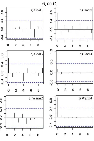
Fig. 2.11 Cross-correlation plots of food conversion rate Cr on growth rate

Fig. 3.1 Plot of the energy balance function E(B,T) when parameterised for individuals reared at 15°C, 20°C and 25°C with data obtained from Experiment 1. By definition, threshold body mass B* is reached when

E(B,T) = 0. Where A is the size at hatching and m is a growth rate coefficient, beyond a critical body weight B* achieved at age t* (where

* mt

Ae *

B = ), it follows that an individual would be unable to support its total energy expenditure. Grist and Jackson (2004) hypothesised that a shift from exponential growth would then be necessary. ... 56

Fig. 3.2 a) Respirometer design and b) experimental setup for the oxygen consumption experiment... 61

Fig. 3.3 Oxygen consumption M as a function of body weight B for juvenile O. pallidus at 18°C. ... 62

Fig. 3.4 Plots of individual growth curves for O. ocellatus at a) 20°C (n = 5) and b) 25°C (n = 5), and O. pallidus at c) 14.7°C (n = 4) and d) 16.9°C (n = 3). The solid black lines, estimated from nonlinear mixed-effect models, represent the mean growth curve for the initial growth phase and the black dots represent the mean transition age and body mass (± 95% confidence interval) out of the exponential growth phase... 64

Fig. 3.5 Plots of the feeding rate coefficient q1 (solid line) and the growth

rate coefficient q3 (dashed line) as a function of temperature T for (a) O. ocellatus and (b) O. pallidus. For each species, symmetric or asymmetric inverted parabolic curves were used to describe q1(T) and q3(T) across the

thermal range in encountered in nature. ... 68

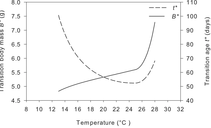
Fig. 3.7 Plot of the model threshold body mass B* and transition age t* as a function of environmental temperature T for O. ocellatus. ... 76

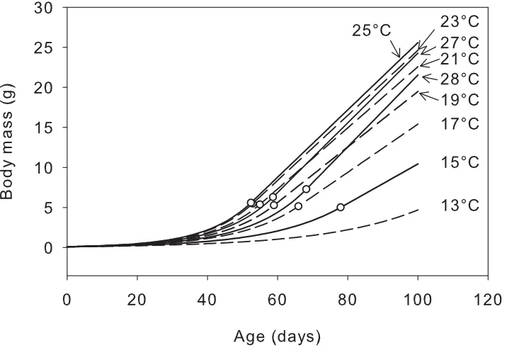
Fig. 3.8 Projected growth trajectories at selected environmental temperatures for O. ocellatus. Circles indicate the transition point (t*, B*) for each individual. ... 77

Fig. 3.9. Elasticity to small perturbations in feeding (Fopt, Topt, df), metabolism (a2, b2, p2) and growth (mopt, Topt, d) rate parameters of a) B* and b) t* at 15°C, 20°C, 25°C and 28°C for O. ocellatus. ... 78

Fig. 4.1 Schematic representation of the modeling approach used to estimate individual growth trajectories. The purpose of the model was to investigate the relative influence of environmental temperature, food consumption, hatching size and inherent growth capacity (marked with a star) on size-at-age in immature octopus... 93

Fig. 4.2 Hatchling size distribution used in the model for Octopus pallidus

in a) summer, b) autumn and c) winter. The distributions were estimated statistically (see Materials and Methods section) and were described by a lognormal distribution A~L

( )

( )

the distribution. Plot d) shows the estimated and observed June hatchling size distribution. ... 99

Fig. 4.3 Estimation of seasonal hatchling size distributions parameters: a) Relationship between incubation time (incubdays) and mean of the hatchling size distribution (A), b) Relationship between mean hatchling

size (A) and variance (s2) used to estimate the summer, autumn and

winter hatchling size distributions. ... 100

Fig. 4.4 Plot of the exponential growth rate coefficient m as a function of temperature T. Inverted parabolic curves of the form 2

) T T ( d m

y= _opt − _opt −

the model by randomly selecting an mopt value from a uniform distribution

U(min_mopt, max_mopt) and assigning the resulting m(T) curve (e.g. dotted

line) to each hatchling at the start of the simulation. ... 102

Fig. 4.5 Plot of the projected individual growth trajectory (here a two-phase growth pattern) of a summer-hatched individual parameterised with an initial hatchling size A=0.194 (g), optimum growth rate mopt=0.083

(day-1_{) and optimum feeding rate f}

opt=1.49 (kj.day-1). ... 104

Fig. 4.6 Simulated size-at-age (with both optimum growth rate mopt and

hatchling size A randomised) for immature Octopus pallidus (n = 200) hatched in a) summer, b) autumn and c) winter. Thin solid lines represent the 5th _{percentile, dotted lines the 95}th _{percentile, dashed lines the 25}th _and

75th _{percentile, thick solid lines the median and solid grey lines the}

number of immature individuals left in the model. Circles represent the size-at-age data of wild individuals from the Bass Strait fishery... 109

Fig. 4.7 Simulated body mass distributions (with both optimum growth rate mopt and hatchling size A randomised) for summer-, autumn- and

winter-hatched Octopus pallidus (n = 200) at a) 60, b) 120 and c) 140 days. Seasonal mean body mass are represented with triangles. Note the different x-axis scale for fig. a). Also, note that at 90 and 120 days, some individuals in the summer and autumn simulations had already reached maturity (607 g)... 111

Fig. 4.8 Simulated size-at-age for immature Octopus pallidus (n = 200) hatched in summer. The relative influence of individual variability was investigated by fixing hatchling size and randomising growth capacity (A

fixed model, black lines), and by fixing inherent growth capacity and randomising hatchling size (mopt fixed model, grey lines). Thin solid lines

represent the 5th _{percentile, dotted lines the 95}th _{percentile, thick solid lines}

cohorts encompassed all the size-at-age data of wild individuals and were not presented here for conciseness. ... 113

Fig. 4.9 Simulated body mass distributions (with both optimum growth rate mopt and hatchling size A randomised) of 200 summer-hatched (a, b, c),

autumn-hatched (d, e, f) and winter-hatched (g, h, i) Octopus pallidus at 60, 90 and 120 days under various food availability (fopt =0.876 to 2.336). Note

that fig. a), d) and g) are on different scales. Also note that at 90 and 120 days, some individuals in the summer and autumn simulations had already reached maturity (607 g). ... 114

Fig. 5.1 Diagram of the life cycle of Octopus pallidus, showing the various stages and the corresponding size classes. Probabilities aj,i correspond to the probabilities of an octopus moving from stage i to stage j during the projection interval and F represent the fecundity of each mature stage.. 131

Fig. 5.2 Population projection matrix P for Octopus pallidus, based on the life cycle diagram in Fig. 5.1. All post-hatch transition probabilities aj,I (in light grey) were determined using the bioenergetics model, while egg to hatchling transition probabilities (in dark grey) were calculated using the projected incubation times. Fecundities F (in black) were determined using reproductive data from wild octopus in Bass Strait... 132

Fig. 5.3 Map showing the western Bass Strait sector to which the downscaling of the sea surface temperature (SST) predictions in 2070 under the A1FI climate change scenario was applied. Data provided by CSIRO (Alistair Hobday, Climate Adaptation Flagship). ... 134

Fig. 5.5 Predicted seasonal hatchling size distributions in 2005, 2030, 2050 and 2070 in a) summer, b) autumn, c) winter and d) spring. Hatchling size was described by a lognormal distribution A~L

( )

( )

Fig. 5.6 Estimated mean body mass at maturity

( )

bivariate normal distribution

(

)

(

)

2

2 _.139

Fig. 5.7 3-D and 2-D representations of the bivariate normal distributions of Inherent growth capacity (mopt) and body weight at sexual maturity (Bmat) for the years a) and b) 2005, c) and d) 2030, e) and f) 2050, and g) and h) 2070. ... 141

Fig. 5.8 Diagram representing the method for estimating yearly seasonal transition probabilities matrices from the 2005, 2030, 2050 and 2070 seasonal transition probabilities matrices. The interpolation is a simple linear change between the estimated proportions... 144

Fig. 5.9 Estimated relationship between body mass in mature females and number of eggs using a type II regression. Circles represent data on 155 wild mature females from the Bass Strait region, taken between 2004 and 2006. White triangles represent the mean body weight for the mature stage. Data courtesy of Stephen Leporati... 147

Fig. 5.10 Relationship between mean incubation temperature and egg survival for O. pallidus (adapted from the egg survival curve of Loligo gahi

by Cinti et al. (2004)). ... 148

Fig 5.12 Seasonal population abundance under the CC scenario for various levels of survivorship: a) 4.5% minimum/65% maximum survival curve, b) 4.5% minimum/73% maximum survival curve, c) 4.5% minimum/75% maximum survival curve, d) 4.5% minimum/77% maximum survival curve and e) 4.5% minimum/85% maximum survival curve... 153

Fig 5.13 Seasonal abundance of a) eggs, b) hatchling stage J3, c) juvenile stage J6, d) mature stage M2 and e) post-spawning stage PS under the CC scenario with a 4.5% minimum/75% maximum survival curve... 157

Fig. 5.14 Diagram of Octopus pallidus life cycle under a) the population exponential phase (CC scenario), b) the population exponential decline phase (CC scenario), c) the end phase (CC scenario), and d) the noCC scenario. Only the most significant seasons and stages are represented (i.e. eggs, hatchling J3, juvenile J6, mature females M1 and M2, post-spawning individuals PS). The intensity of the colour represent the periods of peak abundance (dark = abundant; light = low numbers). Survivorship was set as a 4.5% minimum/75% maximum survival curve... 159

Fig. 5.15 Seasonal population structure for selected years under the CC scenario and a 4.5% minimum/75% maximum survival curve. Colours represent the proportion of each stage in the population and plain lines represent the total population size in the selected year... 161

Fig. 5.16 Seasonal population structure for the mature stages in selected years under the CC scenario and a 4.5% minimum/75% maximum survival curve. Colours represent the proportion of the three mature stages in the mature female population and plain lines represent the number of eggs in the selected year... 162

Fig. 5.18 Seasonal population structure for selected years under the noCC scenario and a 4.5% minimum/75% maximum survival curve. Colours represent the proportion of each stage in the population and plain lines represent the total population size in the selected year... 166

Fig. 5.19 Seasonal population structure for the mature stages in selected years under the noCC scenario and a 4.5% minimum/75% maximum survival curve. Colours represent the proportion of the three mature stages in the mature female population and plain lines represent the number of eggs in the selected year... 166

Fig. 5.20 Sensitivity of the population size through time to a 1% increase and 1% decrease in survivorship across all stages (based on the 4.5% minimum/75% maximum survival curve) under the CC scenario and the noCC scenario. Sensitivity at -1% for both scenarios were confounded.. 167

List of Tables

Table 2.1 Individual IDs, lineage (mother A or B), hatch weight, survival time and temperature treatment for the eight O. pallidus hatchlings reared in the experiment for 143 days. Warm4 was kept another 45 days beyond the experiment. ... 25

Table 3.1 Parameter values for the temperature-dependent energy balance model. B is the body weight of the octopus (g), T the temperature (°C),... 58

(pal) _{indicates references for O. pallidus and} (oc) _{references for O. ocellatus... 58}

Table 3.2 Feeding rate and growth parameters with associated standard errors estimated by nonlinear mixed effect models for O, ocellatus and O. pallidus. ... 66

Table 3.3 Comparison of observed (obs.) with simulated (sim.) transition body mass B* and transition age t* for O. ocellatus and O. pallidus. ... 75

Table 4.1 Equations and parameter values for the dynamic temperature-dependent energy balance model (DTEBM). A is the hatchling size, t is the age (in days) and thatch the hatching day in a 365 day year... 95

Table 4.2 Predicted incubation time in Bass Strait waters (based on an incubation duration of 1067.5 degree-days) and mean of the hatchling size distribution for O. pallidus. The (*) represent observed data for pale octopus. ... 101

Table 4.3 Influence of food availability (expressed as fopt) on the

Table 5.1 Equations and parameter values for the modified dynamic temperature-dependent energy balance model (DTEBM). A is the hatchling size, t is the age (in days) and thatch the hatching day in a 360 day

year. ... 143

Table 5.2 Sequence of modelling under the climate change scenario (CC).

P corresponds to one of 264 projection matrices, S the survival matrix and

N(t) the population at time t. ... 145

Table 5.3 Sequence of modelling under the no climate change scenario (noCC). P corresponds to one of four projection matrices, S the survival matrix and N(t) the population at time t... 145

Table 5.4 Survivorship by stage used in the elasticity analysis. Survivorship was calculated as a ±1% change in survival at each stage, based on the 4.5% minimum/75% maximum survivorship curve... 151

List of Equations

C

h

1

CEPHALOPODS: ROLE AND CHARACTERISTICS

Fig. 1.1 Global landing of cephalopods from 1950 to 2005. Data include commercial, industrial, recreational and subsistence purpose catches (sourced from the FAO Global Production Statistics).

curve is still subject to considerable debate. A variety of models have been fitted to growth data, including power, linear, exponential, sigmoidal, part parabolic and cyclic (see Semmens et al. 2004; and Arkhipkin and Roa-Ureta 2005 for a review). Although it is yet to be demonstrated for wild animals, studies have shown that individuals reared in captivity generally exhibit two-phase growth consisting of an initial rapid exponential phase followed by a slower second power growth phase close to linear, which ends abruptly at the end of the life cycle (DeRusha et al. 1987; Forsythe and Hanlon 1988; Forsythe and Hanlon 1989; Forsythe et al. 2001b; Segawa and Nomoto 2002). In some species, the slower growth phase is better represented by an exponential (Hatfield et al. 2001; Hoyle 2002) or true logarithmic (Cortez et al. 1999a; Ribgy 2004) model.

PLASTICITY AND POPULATION DYNAMICS

hatchlings due to lower yolk reserves in the eggs (e.g Euprymna tasmanica, Steer et al. 2004). Low temperatures or under-nutrition early in the life cycle can result in slow growth (Segawa 1990; Hatfield et al. 2001; Jackson and Moltschaniwskyj 2002; Segawa and Nomoto 2002; Semmens et al. 2004) and/or delayed maturity (Forsythe and Hanlon 1988; Forsythe et al. 2001b), with these factors resulting in larger adult size and longer life spans (Jackson 2004). Under-nutrition or low food availability during the later phases of the life cycle however can induce cephalopods to reproduce earlier at smaller sizes (Mangold 1987).

biomass change very rapidly over short time scales (Grist and des Clers 1998).

Much of our understanding of cephalopod growth, maturation, physiology and energetics is derived from controlled laboratory studies. Although these are essential and have been invaluable in assessing the impact of environmental factors on cephalopod life history, they do not necessary reflect the conditions experienced by individuals in the wild. Despite the major impact of temperature on cephalopod life history, with the exception of Leporati et al. (2007) and Hoyle (2002), captive experiments have only used fixed temperature regimes to investigate the impact of temperature on life history characteristics of cephalopods, and there is little information regarding the impact of dynamic temperatures, as would be experienced in nature.

variable and any improvement in our understanding of environmental impact on cephalopod early life history in the wild would be beneficial.

CEPHALOPODS AND CLIMATE CHANGE

2070 under the A1FI scenario (CSIRO 2007), coastal water temperatures in Tasmania are expected to rise, in the same time period, between 1.4ºC to 4.1ºC due to Tasmania’s complex current system.

As cephalopods adapt rapidly to varying environments and appear to thrive in warmer conditions due to accelerated growth and their opportunistic nature, it has been suggested that cephalopods will prosper with climate change, providing there is sufficient food availability (Bildstein 2002). However, higher temperatures also lead to smaller hatchlings and potentially smaller adults (Pecl et al. 2004b), implying that hatchling size and post-hatching growth rate will likely be opposing forces acting on the size at age of adult cephalopods (Pecl and Jackson 2008). As temperature also has a direct effect on cephalopod metabolism, as well as that of their prey and predators, climate change is certain to have consequences for species abundance and activity rates (Bailey and Houde 1989).

ocean acidification could result in a pH range of 7.15 to 7.95 under the highest emission scenario. In cephalopods, oxygen binding and blood transport is extremely sensitive to changes in pH (Miller and Mangum 1988; Pörtner et al. 2004). Therefore the acidification of oceanic waters is likely to limit oxygen uptake in many species, with consequences for activity rates, growth, reproduction and survival (Seibel and Fabry 2003; Rosa and Seibel 2008). Due to their high rates of activity and elevated metabolism, squids are more likely to be affected than octopus and cuttlefishes (Zielinski et al. 2001), whose blood oxygenation only becomes markedly affected at a water pH<7.4 (Sepia officinalis, Zielinski et al. 2001) and pH<7.2 (Octopus dofleini, Miller and Mangum 1988) respectively against pH<7.5 for squids (Illex illecebrosus, Pörtner and Reipschläger 1996).

(Arntz et al. 1988; Jackson and Domeier 2003; Ish et al. 2004; Zeidberg et al. 2006; Chen et al. 2007).

Other predicted consequences of climate change include modification of the patterns of ocean stratification and/or deep-ocean circulation, changes in the productivity and location of upwelling areas, as well as in the intensity of many currents (Mann and Lazier 2006), which would have consequences for nutrient availability and the distribution of migratory species and those with planktonic stages (paralarvae). Climate change will also bring about modifications in biogeography, as poleward shifts in the range of many species are expected. Such migrations to more suitable thermal environments have already taken place, with the appearance of subtropical and tropical species in temperate areas, such as the observations of the squid Alloteuthis africana and the common paper nautilus Argonauta argo in Spanish waters (Guerra et al. 2002). For completely benthic species, which include some octopus and cuttlefishes, the lack of larval dispersion by means of currents and the limited movement capacities of adults might prove problematic under changing temperature conditions, and animals may be forced to undergo shifts in their depth distribution to match their thermal preferences.

of population dynamics that is required to make predictions is lacking for most cephalopod species. Importantly, understanding population dynamics requires a sound knowledge of the characteristics of the individuals constituting the population (Vanoverbeke 2008), in particular the mechanisms dictating individual growth and how biotic and abiotic factors influence developmental and reproductive processes in the wild. This knowledge is currently lacking and is the focus of the present research.

AIMS AND THESIS STRUCTURE

The ultimate aim of this study is to predict the potential impact of climate change on a cephalopod population with limited dispersal capacity. This is achieved by firstly exploring the early life-history processes in juvenile octopus, and subsequently developing bioenergetic models describing growth and maturation as a function of the main biotic (size, individual variability, nutrition) and abiotic (environmental temperature) factors influencing cephalopod life history. Finally, the population is projected through to 2070 according to the climate predictions of the International Panel for Climate Change (IPCC 2007).

second holobenthic octopus, Octopus ocellatus, were also used to validate the basic bioenergetic model.

The thesis is organized into four data chapters (2-5) culminating in a general discussion (chapter 6). The primary aims and topics addressed in each of the data chapters are as follows:

Chapter 2: The early life-history processes: relationships between temperature, feeding, food conversion, and growth

This chapter explores the early-life history of Octopus pallidus through a captive experiment. Since initial growth is exponential, early life-history is critical in determining future growth trajectories. The specific aim was to investigate, at the individual level, the relationship between early growth and the significant factors affecting growth, namely food intake, food conversion and fluctuating environmental temperatures. The feeding and growth data collected in this chapter form the basis on which the bioenergetic models developed in the following two chapters were built. This research is published in: Journal of Experimental Marine Biology and Ecology (2008) 354: 81-92 (see Appendix).

Chapter 3: Modelling the impact of temperature on the growth pattern of octopus using bioenergetics

Octopus pallidus growth data in captivity. The model is then employed to investigate growth patterns occurring at different fixed temperatures for both species.

This research is published in: Marine Ecology Progress Series (2009) 374: 167-179 (see Appendix).

Chapter 4: Modelling size-at-age in wild immature animals: the relative

influence of the principal abiotic and biotic factors

This chapter explores the predicted growth of Octopus pallidus in the wild. The bioenergetics model developed in the previous chapter was modified to include dynamic seasonal temperatures and individual variability in growth and hatchling size, in order to simulate the juvenile growth trajectories of individuals hatched in different seasons. This allows the investigation of the relative influence of the principal biotic (hatchling size, individual variability, nutrition) and abiotic (environmental temperature) factors affecting size-at-age in wild immature Octopus pallidus.

This research is published in: Marine Ecology Progress Series (2009) 384: 159-174 (see Appendix)

Chapter 5: Potential impact of climate change on the Eastern Bass Strait

pale octopus population

In this final data chapter, the western Bass Strait Octopus pallidus

population structure and dynamics is assessed. This is achieved by integrating the results of the individual-based bioenergetic models described previously into a complete matrix population model, therefore accounting for the effect of environmental temperature and individual variability on the biology of O. pallidus (e.g. egg incubation time, growth, reproduction).

STUDY SPECIES

This study focuses on two commercially exploited benthic octopus species,

Octopus pallidus and Octopus ocellatus, with the former being the main focus of the research. Both species belong to the family Octopodidae and are characterized by holobenthic hatchlings as opposed to other larger merobenthic octopus species with planktonic young (paralarvae).

Octopus pallidus (Hoyle 1885)

(Norman and Reid 2000). Populations of this species show very little overlap in generations despite all year round egg-deposition (Leporati et al. 2008b). This species is targeted recreationally throughout its range and commercially in northern Tasmanian waters (Bass Strait region), with catches of 81 tonnes in 2007 (Leporati et al. 2008a).

Octopus ocellatus (Gray 1849)

The gold-spot octopus Octopus ocellatus is a small benthic octopus (less than 100g) with a life span of 6 to 12 months depending on geographical location (Segawa and Nomoto 2002). Gold-spot octopus inhabit the shallow waters from the southern coast of Hokkaido to the Chinese continent and southern Korean Peninsula (Okutani et al. 1987), preferring sandy and muddy habitats (Fig. 1.3). Female O. ocellatus lay 300 to 400 large eggs (7 mm length) in crevices and empty shells, which develop into benthic hatchlings (Yamoto 1941a; Yamoto 1941b). Thegold-spot octopus is important in both commercial and recreational fisheries along the Japanese coast especially in Tokyo Bay and the Seto Inland Sea (Segawa and Nomoto 2002).

ANIMAL ETHICS

Octopus ocellatus

Octopus pallidus

The early life-history processes:

relationships between

temperature, feeding, food

conversion and growth

This Chapter previously published as:

André J, Pecl GT, Semmens JM and Grist EPM (2007) Early life-history processes in benthic octopus: relationships

between temperature, feeding, food conversion, and growth in juvenile Octopus pallidus. Journal of Experimental Marine Biology and Ecology 354: 81-92

C

h

ABSTRACT

INTRODUCTION

In common with other cephalopods, individual growth in octopus is

highly variable, even within groups of siblings reared under identical

conditions (Van Heukelem 1976; Forsythe and Van Heukelem 1987).

Numerous biotic and abiotic factors can influence growth, including

temperature (Forsythe and Hanlon 1988; Forsythe 1993; Pecl 2004), food

quality and quantity, age, size, gender, stage of maturity and level of

activity (Forsythe and Van Heukelem 1987). In the juvenile phase,

temperature (Forsythe and Van Heukelem 1987), food ration (Villanueva

et al. 2002), food quality (Villanueva 1994) and hatchling size (Leporati et

al. 2007) appear to have the most significant impact on growth. Higher

temperatures result in higher growth rates for octopus with both benthic

(Forsythe and Hanlon 1988; Segawa and Nomoto 2002) and planktonic

(Itami et al. 1963; Villanueva 1995) hatchlings, as well as for deep-sea

octopus (Wood 2000). However, most studies have only used one or

several fixed temperature regimes to investigate the impact of temperature

on growth, with only Leporati et al. (2007) having explored the effect of

seasonal temperatures on the growth of octopus hatchlings. There is in

general little information regarding the impact of dynamic temperatures,

as would be expected in nature, on the physiology of cephalopods.

Variability in individual food conversion may also contribute to

efficiency) is highly variable between individuals even for octopus reared

on the same diet (Mangold and von Boletzky 1973). High levels of activity,

low food intake (Wells and Clarke 1996) and sexual maturity (Mangold

1983a; Mangold 1983c; Klaich et al. 2006) are known to lower food

conversion since less energy is available for somatic growth. Food

conversion, however, appears independent of sex (Hanlon 1983; Forsythe

1984) and body size (Mangold 1983a). It also appears independent of

temperature in some species (Octopus vulgaris, Mangold and von Boletzky 1973; Eledone moschata, Mangold 1983a), but not in others (Octopus tehuelchus, Klaich et al. 2006). Gross growth efficiency (food conversion rate) appears variable at the individual level, exhibiting apparent periodic

fluctuation over time in some species (Mangold and von Boletzky 1973;

Mangold 1983a; Mangold 1983c) although the cause of these fluctuations

has not been established.

The objective of this chapter was to examine the relationship between

growth in juvenile octopus and significant factors affecting growth,

namely food intake, food conversion and temperature. Individual feeding

rate, food conversion rate, and growth rate were determined for pale

octopus hatchlings reared under identical nutritional conditions but two

different dynamic temperature regimes. As octopus initially grow

exponentially, the early life-history is critical in determining their growth

cycle, except in a few commercial species (Segawa and Nomoto 2002;

Iglesias et al. 2004). This chapter aims to improve the current

understanding of the growth processes in juvenile octopus.

MATERIAL AND METHODS

Study animals and experimental design

Two brooding females (designated as females A and B) were collected in

March 2005 from the commercial pot fishery in north-west Tasmania,

Australia (40° 49.268; 145° 39.774 west and 40° 50.240; 145° 42.091 east, 45

meters depth). Animals were maintained in separate 250 litre tanks in an

indoor system at ambient sea temperature (22−11°C from March to July) until the eggs hatched. The first hatching occurred 123 days after

collection.

After an acclimatisation period of 24 hours, hatchlings were placed in

individual two litre containers fitted with mesh sides to allow water flow

and a scallop shell for shelter. The containers were kept in 250 l stock

tanks under a fluorescent lighting regime which replicated natural

daylight variation (06.00−18.00 hrs light, 18.00−06.00 hrs dark). Two temperature regimes were established: a warmer temperature regime

(increasing from 16°C to 18°C over a period of 36 days then stable at 18°C

14°C over a period of 36 days then stable at 14°C for 107 days).

Temperature was altered by 1°C on day 18 and day 36 of the experiment

(Fig. 2.1), and temperature in the tanks was recorded every 15 mins by two

data-loggers (StowAway Tidbit, USA, http://www.onsetcomp.com).

Fig. 2.1 Intended ( --- ) and actual ( ─ ) temperature regimes recorded

during the experiment. Standardised (std) temperature used in the time series analysis (see Data analysis section p. 28)are represented by circles for the cool regime and squares for the warm regime.

Four randomly selected day-old hatchlings (two from female A and two

from female B all born on 19/07/05) were held under each temperature

regime. Individuals were designated as octopus Cool1 to Cool4 and

Warm1 to Warm4 according to their temperature regime (Table 2.1).

Growth and food intake was individually monitored for a period of 143

Table 2.1 Individual IDs, lineage (mother A or B), hatch weight, survival

time and temperature treatment for the eight O. pallidus hatchlings reared in the experiment for 143 days. Warm4 was kept another 45 days beyond

the experiment.

Growth, food consumption, and food conversion rate

Individuals were weighed every 5 to 10 days and the instantaneous

growth rate Gr, expressed as the percent increase in body mass per day, was calculated using the standard exponential growth formula:

100 ln

ln

1 2

1 2 _×

− − =

t t

B B

G_r (1)

where B1 and B2 are body masses (g) at time t1 and t2 (Forsythe and Van Heukelem 1987).

best fit model was chosen on the basis of the highest adjusted r2 _values (DeRusha et al. 1987; Hatfield et al. 2001). Adjusted r2 _{values were} calculated by linear regression to B versus t for the linear model, log(B) versus t for the exponential model, and log(B) versus log(t) for the power model. Average growth for each temperature treatment was calculated as

the mean of individual growth equation parameter values.

All individuals were fed porcelain crabs (Petrolisthes elongatus) collected from around the Hobart area (Tasmania). Two live crabs, whose relative

body weight totalled between 4% and 12% of the octopus body weight,

were supplied daily to each animal. The level of food offered was

comparable to the level of food consumed by other octopus species reared

in captivity under ad libitum condition (Joll 1977; Mangold 1983b; O'Dor and Wells 1987). Before being fed to each individual octopus, crabs were

dried with absorbing paper and weighed on a digital scale to 0.001g

accuracy. Uneaten crab remains from the previous day were removed

from each container and frozen immediately for later analysis. Any live

uneaten crab was removed and weighed.

After defrosting, remains were washed three times with ammonium

formate (0.5 M) to remove any salts before being dried in an oven for 24

hours at 60°C. The samples were then placed in a desiccator for one hour

to remove any moisture and weighed on a digital scale to 0.0001g accuracy.

randomly selected samples of remains in order to calculate the ww/dw

conversion factor.

The quantity of food consumed in a given day D was:

r u

f w w

w

D= − − (2)

where wfdenotes the wet weight (g) of live crabs fed to the octopus, wu denotes the wet weight (g) of any live crabs uneaten the next day and wr denotes the wet weight (g) of remains from eaten crabs.

The weight specific feeding rate Fr expressed as a percentage of body mass per day was calculated according to Houlihan et al. (1998):

100 × × = t B D F m t

r (3)

where t is the number of days between two weighings, Dt is the amount of food (g wet weight) consumed over the time interval t, and Bm is the mean body weight (g wet weight) of the octopus over the time interval t.

Food conversion (%) expresses the amount of food intake required to fuel

a unit amount of growth. To explore the relationship with Fr and Gr, we have expressed food conversion Cr as a rate in percentage per day, which we calculated according to a modification of the Mangold and von

Boletzky (1973) formulae:

100 × × ∆ = t D B C t

where ∆B is the difference in body mass (g) between two weighings, t is the number of days between two weighings, and Dt is the amount of food (g wet weight) consumed over the time interval t.

Data analysis

For all averages given, a corrected standard error SE* _{= t × SE, where t is} the t-score, was used where sample size was smaller than 20 (Fowler et al. 1998). Significance level throughout the analysis was set at p <0.05. Time series analysis was performed on individual feeding rate Fr, growth rate Gr, food conversion rate Cr, and temperature T data. Weights were obtained every five to ten days and the resulting time series were standardised in

terms of seven day time steps by the use of linear interpolation.

Accordingly, Fr, Gr, Cr and T were calculated over the same time step. Time series exhibiting linear trends were detrended linearly. Time series

(Fr, Gr and Cr) were first analysed separately using autocorrelation plots to assist with identifying any cycles. Since data were in weekly time steps,

lag 1 corresponded to a time shift of seven days, lag 2 a time shift of 14

days and so on. Where a significant autocorrelation was established, the

time series was further investigated through partial autocorrelation plots.

Partial-autocorrelation measures the strength of the correlation at specific

lag (e.g. lag 4) while removing the effects of all autocorrelations below that

lag (i.e. autocorrelation occurring at lags 0, 1, 2 and 3). Only

2.2) were examined separately using correlation and partial

cross-correlation analyses. Partial cross-correlation coefficients (r) were calculated when significant correlations were established.

Fig. 2.2 Schematic diagram of the relationships between temperature T,

feeding rate Fr, growth rate Gr and food conversion Cr investigated in this chapter.

To assess the direction of influence (e.g. if changes in x caused changes in

y, or the opposite), time series x were time-shifted against y both forward (showing the effect of x on y, referred to as plots of x on y) and backward (showing the effect of y on x, referred to as plots of y on x). Given the relatively short lengths of all time series (20 data points), cross-correlations

and partial cross-correlation analysis beyond a lag 6 (42 days) were

considered to be redundant in view of the likelihood of type I and type II

errors occurring at higher lags. The mean Fr, Gr and Cr time series were also calculated for each temperature regime and analysed as previously

for individual time series. The software R version 2.2.1 was used to carry

RESULTS

The mean hatch weight (g ± SE*) was 0.231 ± 0.034 for hatchlings from female A (range= 0.206 − 0.258 g, n = 4) and 0.275g ± 0.036 for hatchlings from female B (range= 0.251 − 0.303 g, n = 4). Octopus did not appear stressed (inking and jet escape movement were rarely seen) and spent

most of their time sheltering under the scallop shell. Little movement was

observed and so the level of activity was considered minimal. The survival

rate over the durarion of the experiment was 75%, with two octopus

reared under the warm treatment (Warm1 and Warm3) dying for

unknown reasons at 57 and 94 days respectively after hatching. Data for

these individuals were discarded in this chapter because there were too

few data points to establish sufficiently long individual feeding and

growth data series.

Temperatures in the two treatments fluctuated more than originally

intended due to mechanical failures of the heater/chiller units (Fig. 2.1).

The treatments nevertheless followed the intended main trend of

increasing (warm) and decreasing (cool) temperature with time. These

shorter term temperature fluctuations were an integral part of the

Food consumption, food conversion rate, and growth rate

All octopus started feeding within hours after hatching, preying on the

smallest size crabs (2mm carapace length). Five out of the six individuals

exhibited at least one subsequent period of “starvation” (ranging from 1 to

7 days) in which they did not eat and lost weight. In general, daily food

consumption D increased with body weight. The mean D (g wet weight ±

SE) for the warm regime was 0.024 ± 0.002 and 0.020 ± 0.001 for the cool treatment.

The mean feeding rate (% body weight per day ± SE) was 2.87 ± 0.16 for octopus reared under the warm treatment (range = 0.79 − 5.69% body weight.day-1_{, n = 40), and 2.45} ± _{0.12 for octopus reared under the cool} treatment (range = 0.10 − 5.93% body weight.day-1_{, n = 80). Although} fluctuations appeared regular in these standardised time series (Fig. 2.3),

Fig. 2.4 Autocorrelation plots of the average feeding rate Fr (in % body weight per day) under a) the cool temperature regime (n = 4), and b) the warm temperature regime (n = 2). Bars that protrude beyond the dotted lines indicate significant correlations.

Food conversion rates Cr were variable from one week to the next (Fig. 2.5), ranging from -8.10 to 70.40%.d-1 _{under the warm regime (mean % per day}

± SE = 9.57 ± 1.93, n = 40) and from -6.30 to 23.90%.d-1 _{for octopus reared} under the cool treatment (mean = 8.61 ± 0.67, n = 79). Cr could not be calculated for Cool4 between day 136 and 143 since this individual

consumed no food during this period. Food conversion rate is however

expected to exceed 100%.d-1 _{for that period since substantial growth was}

observed despite the lack of food intake. Only individual Warm2

displayed evidence of periodicity in food conversion rate with a highly

Fig. 2.6 a) Autocorrelation plot of food conversion rate for Warm2; b)

autocorrelation plot of growth rate for Cool4. Bars that protrude beyond the dotted lines indicate significant correlations.

Individual growth under both temperature regimes was best described by

an exponential curve (Fig. 2.7) with adjusted r2 _{values for individual} growth trajectories ranging between 0.91 and 0.99. The mean best fit

growth curve was B = 0.227e0.015t _{under the warm regime and B =} 0.264e0.013t _{under the cool regime. Octopus under the warm regime}

(growth rate m = 0.015) grew faster than those under the cool regime (m = 0.013). Warm4 exhibited a two-phase growth pattern in which a striking

change in body weight occurred at around 133 days (Fig. 2.7). The

resulting two-phase growth curve is best described by the exponential

0.0 0.5 1.0 1.5 2.0 2.5 3.0 3.5 4.0

0 10 20 30 40 50 60 70 80 90 100 110 120 130 140 150

Age (days) Bo d y w e ig h t ( g )

Average: B= 0.264 e 0.013t

Cool4 Cool3 Cool2 Cool1 (a) 0.0 0.5 1.0 1.5 2.0 2.5 3.0 3.5 4.0

0 10 20 30 40 50 60 70 80 90 100 110 120 130 140 150

Age (days) Bo d y w e ig h t ( g ) (b) Warm2 Warm4

Average: B= 0.227 e 0.015t

Fig. 2.7 Raw data of individual (─) and average (---) growth under the a)

cool and b) warm temperature regime.

In close agreement with the exponential growth rate coefficients m

obtained from the regression models described above, the mean growth

statistically significant periodicity in Gr, with a negative cross-correlation at lag 1 (Fig. 2.6b).

Effect of temperature on Fr, Gr and Cr

Overall, cross-correlation analyses suggested that changes in temperature

did not drive changes in Fr, or Gr or Cr. Analysis of the mean Cr time series for the cool regime showed a significant positive cross-correlation between

T and Cr at lag 0 (r = 0.64) (Fig. 2.8a), suggesting that changes in food conversion rates in the current week were correlated with changes in

temperature. This significant correlation was most likely influenced by

individual Cool4, which displayed a similar cross-correlation pattern with

temperature (r = 0.68 for lag 0) (Fig. 2.8b). The absence of significant cross-correlations for the other five individuals suggests that temperature had a

minimal effect on Cr. No significant cross-correlations were obtained between the mean Fr time series and temperature, or between individual Fr time series and temperature (Fig. 2.8c and 2.8d), suggesting that changes in temperature had no effect on feeding rate. Similarly,

temperature appeared to have no influence on growth rate as revealed by

Feeding rate and growth rate

Interestingly, fluctuations in feeding rate did not appear to drive

fluctuations in growth rate as evidenced by the absence of significant

cross-correlations of Fr on Gr (Fig. 2.9a and 2.9b). Fluctuations in Gr however influenced fluctuations in Fr under the warm regime, with a positive cross-correlation of Gr on Fr at lag 1 (Fig. 2.9c). This significant correlation was most likely influenced by individual warm2, which

displayed a similar cross-correlation pattern (Fig. 2.9d). The absence of

significant cross-correlations for the other five individuals suggests that

the effect of Gr on Fr is minimal.

Fig. 2.9 Cross-correlation plots showing the relationship between feeding

Feeding rate and food conversion rate

Analysis of the mean time series showed a significant negative

cross-correlation at lag 0 for Cr on Fr under the cool regime (r = -0.68) (Fig. 2.10a). This significant relationship was mainly due to consistent negative

cross-correlations exhibited by all individuals for Cr on Fr at lag 0, even though only that of Cool4 was statistically significant at this lag (r = -0.63) (Fig. 2.10c). The analysis for individual Warm4 also revealed a significant

negative cross-correlation at lag 0 (r = -0.79) (Fig. 2.10e), although no such pattern was evident from the analysis of the mean time series for the

warm regime (Fig. 2.10d). Overall, individuals that demonstrated a high

food conversion rate tended to have a low feeding rate in the same week,

and vice versa. Fluctuations in food conversion rate also appeared to drive

fluctuations in feeding rate in subsequent weeks for some individuals.

Analysis of the mean time series of Cr on Fr for the warm regime revealed a significant positive cross-correlation at lag 3 (Fig. 2.10d). This was

mainly due to positive cross-correlations at this lag exhibited by Warm2

and Warm4, even though none of them was statistically significant.

Analysis of the mean time series of Cr on Fr for the cool regime did not reveal any significant cross-correlations although the analysis for

individual Cool3 revealed a significant positive cross-correlation at lag 4

Interestingly however, the cross-correlation analysis of Fr on Cr revealed that there were no significant correlations for any individual, which

suggests that fluctuations in Cr were not determined by fluctuations in Fr.

Fig. 2.10 Cross-correlation plots showing the relationship between food

Growth rate and food conversion rate

The time series for Gr and Cr supported the existence of a relationship between Gr on Cr with evidence of a positive cross-correlation occurring at a time lag of under a week (lag 0). All individuals but Cool4 had

statistically significant cross-correlations at lag 0 (0.85 < r < 0.97) (Fig. 2.11).

The lack of a significant correlation for this individual can be accounted

DISCUSSION

The relationship between Fr, Gr, Cr and T is highly complex with this detailed study revealing unexpected results such as the lack of a

correlation between feeding rate and growth rate, and the observation that

dynamic temperatures have little effect on any of the variables examined.

Strong individual variability was evident and may in part be explained by

the dynamic growth process.

Food consumption, food conversion rate and growth rate

As for other octopuses reared in laboratory conditions (Nixon 1966;

Mather 1980; Boyle and Knobloch 1982; Houlihan et al. 1998), individuals

did not feed everyday potentially as a consequence of stress in captivity

(Houlihan et al. 1998). Feeding rates were comparable to those of

sub-adult or sub-adult octopus from other species (Boyle and Knobloch 1982;

Mangold 1983a; Houlihan et al. 1998; Segawa and Nomoto 2002) but were

much lower (0.10 to 5.93%.d-1_{) than feeding rates of 18.8 to 32.3%.d}-1 _found

for captive juvenile Octopus ocellatus (Segawa and Nomoto 2002). Mean food conversion rates found for O. pallidus were higher than that reported for immature Octopus tehuelchus (Klaich et al. 2006) another species with benthic hatchlings (4.4%.d-1 _{at 15°C and 5.2%.d}-1 _{at 10°C- calculated from}

fluctuations have been reported in previous studies (Mangold and von

Boletzky 1973; Mangold 1983a; Mangold 1983c). One individual displayed

a Cr in excess of 100%.d-1 which suggests that all the growth observed can not be explained by current or very recent food intake.

Growth trajectories were exponential throughout the experimental period

but animals did not display two-phased growth (exponential growth

phase followed by a slower growth phase) as observed for other cultured

octopus species (Forsythe and Van Heukelem 1987; Semmens et al. 2004).

Growth rates of 1.38% and 1.67% for the cool and warm treatment

respectively were comparable to the values of 1.43% (cool treatment) and

1.73% (warm treatment) found by Leporati et al. (2007) for O. pallidus

hatchlings reared under fluctuating temperature regimes similar to those

employed in this study.

Food consumption, food conversion and growth rates all exhibited

fluctuations over time. These fluctuations showed no statistically

significant periodicity on a weekly basis but may be linked to some

underlying physiological growth mechanism, as discussed further below

(p 47).

Effect of temperature on Fr, Gr and Cr

Temperature is one of the most important abiotic factors affecting the

physiology of poikilothermic animals. The lack of relationship between

food conversion rate and temperature in the present study is consistent

Boletzky 1973; Mangold 1983a) which found that food conversion rate had

no dependence on temperature. Temperature-dependence of growth rate

and feeding rate is, on the other hand, well established for octopus, with

higher temperatures resulting in higher food intake (Mangold and von

Boletzky 1973; Joll 1977; Segawa and Nomoto 2002) and growth (Semmens

et al. 2004) within the thermal range of a species. The lack of statistical

support for a relationship between Fr and temperature or Gr and temperature in this study may be connected with a complex response to

the fluctuating temperature regime. Since maintenance costs are

temperature-related (Wells and Clarke 1996), short-term fluctuating

temperatures would most likely produce variations in maintenance costs

that must ultimately result in variations in growth. This could obscure a

direct dependence of growth on temperature. The substantial variations

observed in food conversion rates could also have contributed to the lack

of a strong relationship between growth and temperature as suggested by

Joll (1977). The pattern observed in this study is however more likely to

reflect the situation in the wild since short-term environmental

temperature fluctuations would be frequently encountered by octopus,

either from individuals moving between deep and shallow waters or

through exposure to different water masses.

Relationship between Fr, Gr and Cr